
Learning Local Distribution for Extremely Efficient Single-Image Super-Resolution

Abstract
:1. Introduction
2. Proposed Method
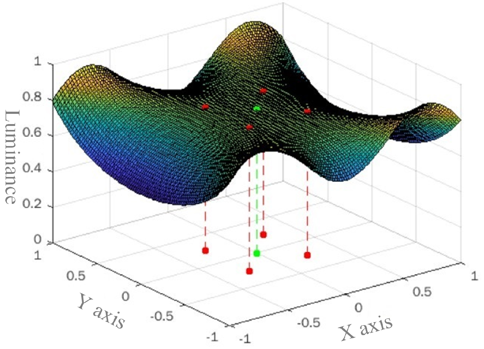
2.1. Motivation
2.2. Local Distribution Reconstruction
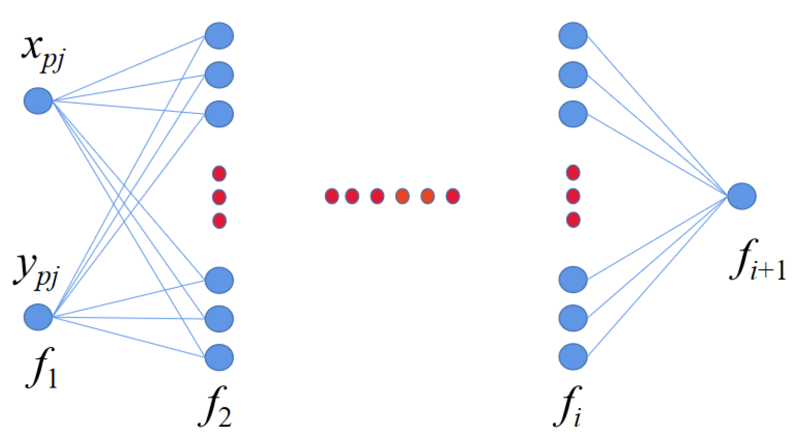
2.3. Sampling Matrix
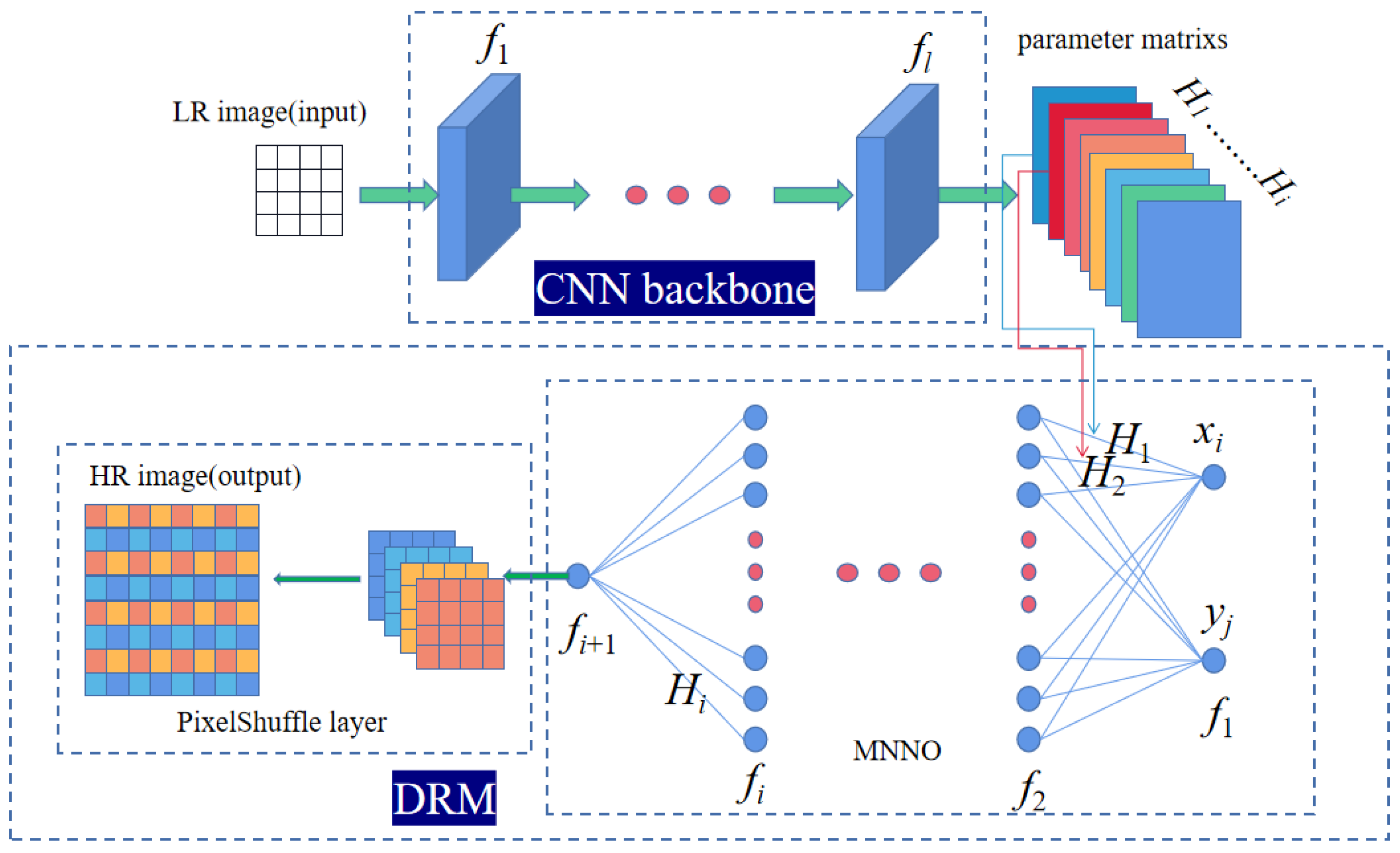
2.4. Overview of the Architecture
2.5. Implementation Details
3. Experiments
3.1. Datasets
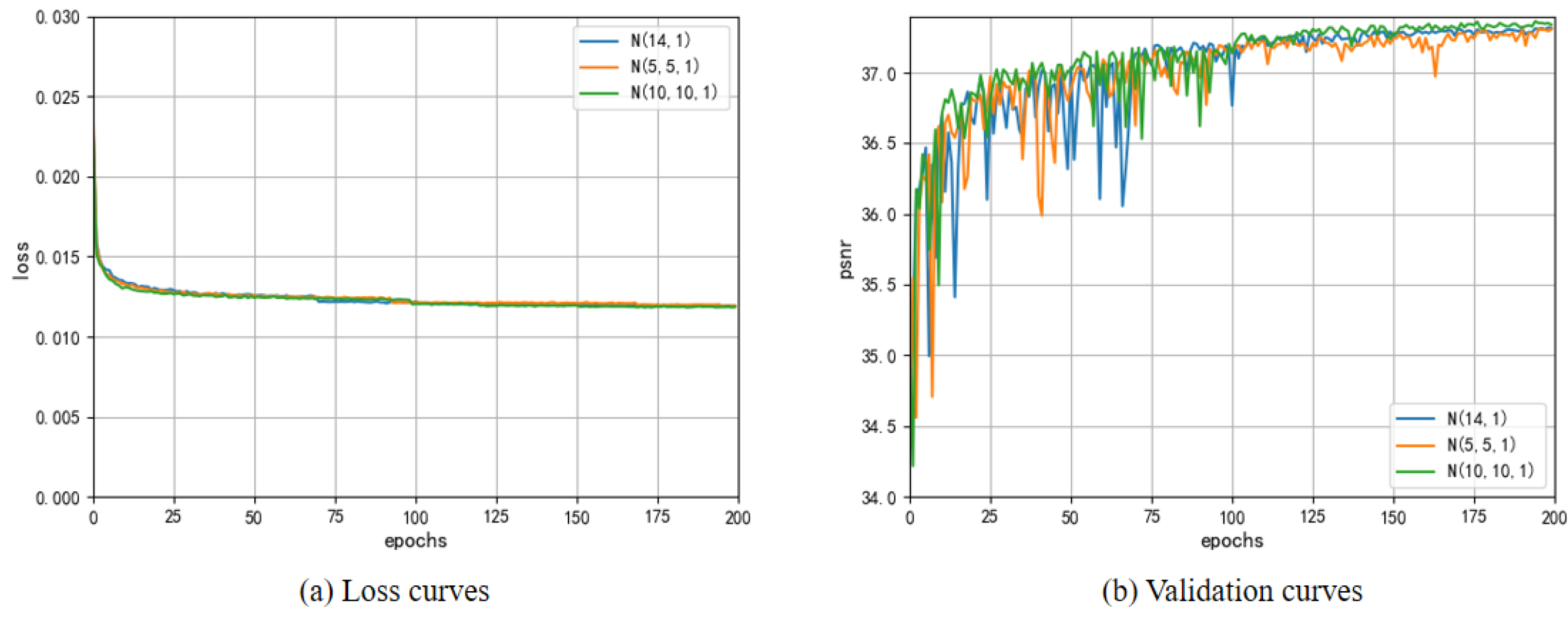
3.2. Ablation Investigation
3.2.1. CNN Backbone
3.2.2. Distribution Reconstruction Module
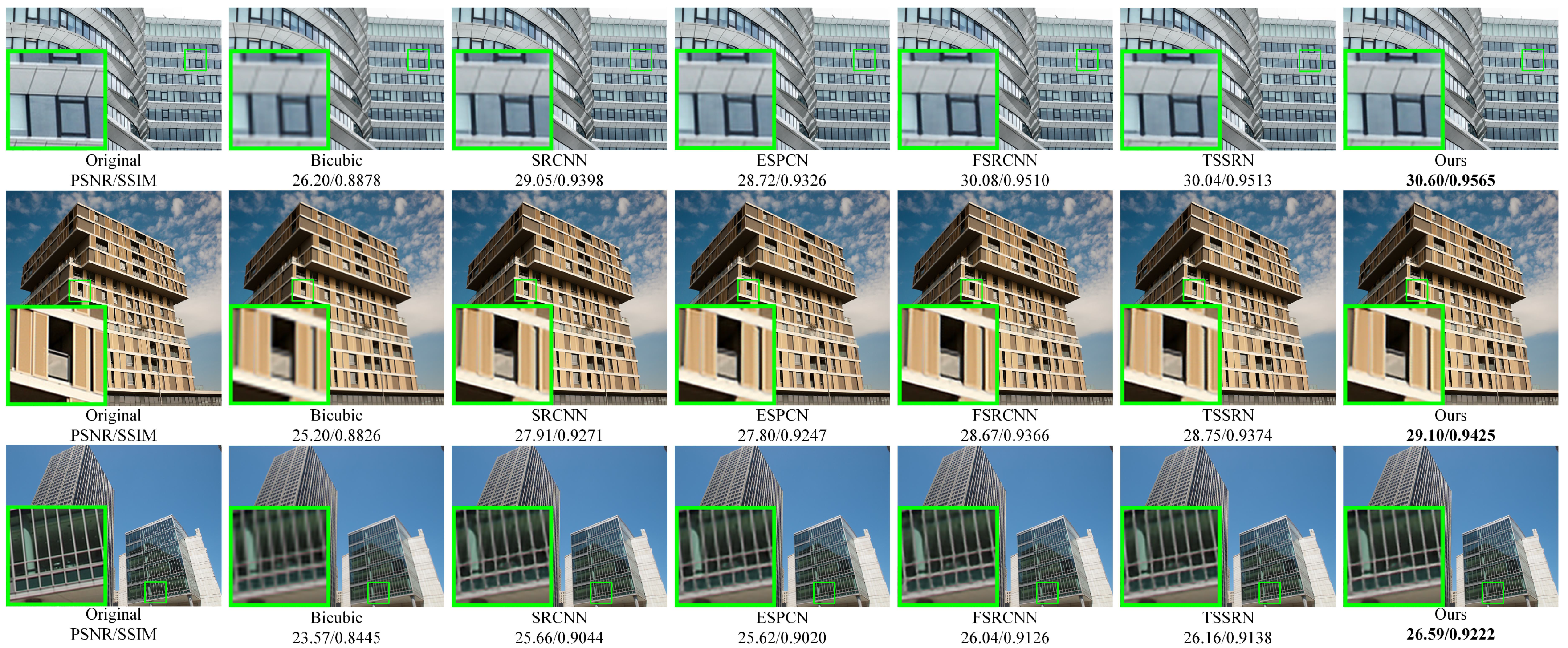
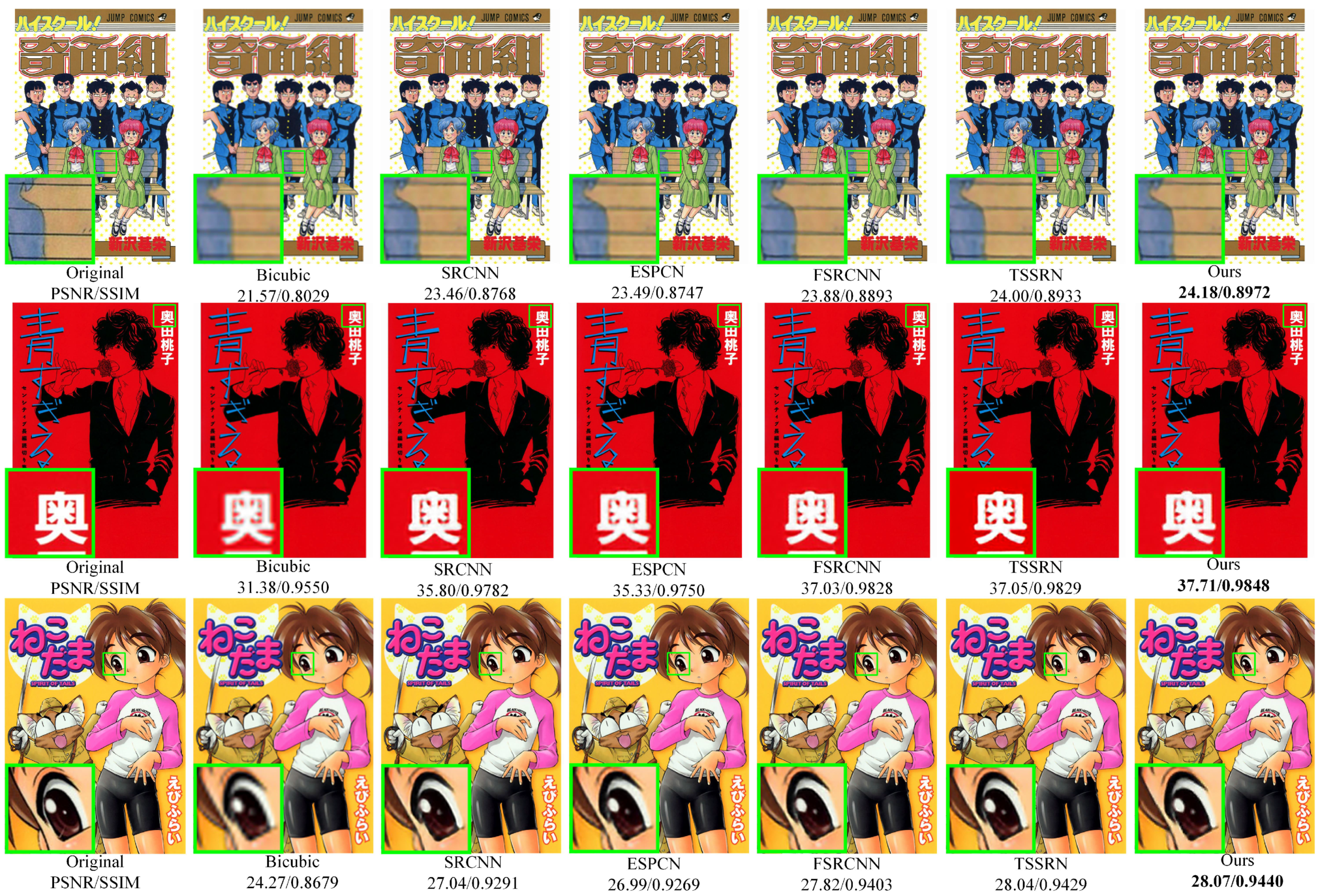
3.3. Comparison with State-of-the-Art Methods
4. Conclusions
Author Contributions
Funding
Institutional Review Board Statement
Informed Consent Statement
Data Availability Statement
Conflicts of Interest
References
- Zhou, F.; Yang, W.; Liao, Q. Interpolation-based image super-resolution using multisurface fitting. IEEE Trans. Image Process. 2012, 21, 3312–3318. [Google Scholar] [CrossRef]
- Gilman, A.; Bailey, D.G.; Marsland, S.R. Interpolation models for image super-resolution. In Proceedings of the 4th IEEE International Symposium on Electronic Design, Test and Applications (Delta 2008), Hong Kong, China, 23–25 January 2008; pp. 55–60. [Google Scholar]
- Mallat, S.; Yu, G. Super-resolution with sparse mixing estimators. IEEE Trans. Image Process. 2010, 19, 2889–2900. [Google Scholar] [CrossRef] [Green Version]
- Chappalli, M.B.; Bose, N.K. Simultaneous noise filtering and super-resolution with second-generation wavelets. IEEE Signal Process. Lett. 2005, 12, 772–775. [Google Scholar] [CrossRef]
- Lo, K.H.; Wang, Y.C.F.; Hua, K.L. Joint trilateral filtering for depth map super-resolution. In Proceedings of the 2013 Visual Communications and Image Processing (VCIP), Kuching, Malaysia, 17–20 November 2013; pp. 1–6. [Google Scholar]
- Mei, Y.; Fan, Y.; Zhou, Y. Image super-resolution with non-local sparse attention. In Proceedings of the IEEE/CVF Conference on Computer Vision and Pattern Recognition, Nashville, TN, USA, 20–25 June 2021; pp. 3517–3526. [Google Scholar]
- Bendory, T.; Dekel, S.; Feuer, A. Super-resolution on the sphere using convex optimization. IEEE Trans. Signal Process. 2015, 63, 2253–2262. [Google Scholar] [CrossRef] [Green Version]
- Ng, M.K.; Bose, N.K. Mathematical analysis of super-resolution methodology. IEEE Signal Process. Mag. 2003, 20, 62–74. [Google Scholar] [CrossRef]
- Sun, L.; Hays, J. Super-resolution from internet-scale scene matching. In Proceedings of the 2012 IEEE International Conference on Computational Photography (ICCP), Seattle, WA, USA, 28–29 April 2012; pp. 1–12. [Google Scholar]
- Qu, Y.Y.; Liao, M.J.; Zhou, Y.W.; Fang, T.Z.; Lin, L.; Zhang, H.Y. Image super-resolution based on data-driven Gaussian process regression. In International Conference on Intelligent Science and Big Data Engineering; Springer: Berlin, Germany, 2013; pp. 513–520. [Google Scholar]
- Dong, C.; Loy, C.C.; He, K.; Tang, X. Learning a deep convolutional network for image super-resolution. In Proceedings of the ECCV, Zurich, Switzerland, 6–12 September 2014. [Google Scholar]
- Yang, S.; Wang, M.; Chen, Y.; Sun, Y. Single-image super-resolution reconstruction via learned geometric dictionaries and clustered sparse coding. IEEE Trans. Image Process. 2012, 21, 4016–4028. [Google Scholar] [CrossRef]
- Gu, S.; Zuo, W.; Xie, Q.; Meng, D.; Feng, X.; Zhang, L. Convolutional sparse coding for image super-resolution. In Proceedings of the IEEE International Conference on Computer Vision, Santiago, Chile, 7–13 December 2015; pp. 1823–1831. [Google Scholar]
- Wang, Z.; Liu, D.; Yang, J.; Han, W.; Huang, T. Deep Networks for Image Super-Resolution with Sparse Prior. In Proceedings of the ICCV, Santiago, Chile, 7–13 December 2015; pp. 370–378. [Google Scholar] [CrossRef] [Green Version]
- Yamashita, R.; Nishio, M.; Do, R.K.G.; Togashi, K. Convolutional neural networks: An overview and application in radiology. Insights Into Imaging 2018, 9, 611–629. [Google Scholar] [CrossRef] [Green Version]
- Yang, X.; Mei, H.; Zhang, J.; Xu, K.; Yin, B.; Zhang, Q.; Wei, X. DRFN: Deep recurrent fusion network for single-image super-resolution with large factors. IEEE Trans. Multimed. 2018, 21, 328–337. [Google Scholar] [CrossRef] [Green Version]
- Hui, Z.; Wang, X.; Gao, X. Two-stage convolutional network for image super-resolution. In Proceedings of the 2018 24th International Conference on Pattern Recognition (ICPR), IEEE, Beijing, China, 20–24 August 2018; pp. 2670–2675. [Google Scholar]
- Ronneberger, O.; Fischer, P.; Brox, T. U-Net: Convolutional Networks for Biomedical Image Segmentation. In Proceedings of the International Conference on Medical Image Computing and Computer-assisted Intervention, Munich, Germany, 5–9 October 2015. [Google Scholar]
- Shi, W.; Caballero, J.; Huszar, F.; Totz, J.; Aitken, A.P.; Bishop, R.; Rueckert, D.; Wang, Z. Real-Time Single Image and Video Super-Resolution Using an Efficient Sub-Pixel Convolutional Neural Network. In Proceedings of the CVPR, IEEE, Las Vegas, NV, USA, 27–30 June 2016. [Google Scholar] [CrossRef] [Green Version]
- Arirangan, S.; Kottursamy, K. Multi-scaled feature fusion enabled convolutional neural network for predicting fibrous dysplasia bone disorder. Expert Syst. 2021, e12882. [Google Scholar] [CrossRef]
- Saranya, A.; Kottursamy, K.; AlZubi, A.A.; Bashir, A.K. Analyzing fibrous tissue pattern in fibrous dysplasia bone images using deep R-CNN networks for segmentation. Soft Comput. 2021, 1–15. [Google Scholar] [CrossRef]
- Lan, R.; Sun, L.; Liu, Z.; Lu, H.; Pang, C.; Luo, X. MADNet: A fast and lightweight network for single-image super resolution. IEEE Trans. Cybern. 2020, 51, 1443–1453. [Google Scholar] [CrossRef]
- Chudasama, V.; Prajapati, K.; Upla, K. Computationally efficient super-resolution approach for real-world images. In Proceedings of the National Conference on Computer Vision, Pattern Recognition, Image Processing, and Graphics, Hubballi, India, 22–24 December 2019; Springer: Berlin, Germany, 2019; pp. 143–153. [Google Scholar]
- Liu, J.; Zhang, W.; Tang, Y.; Tang, J.; Wu, G. Residual feature aggregation network for image super-resolution. In Proceedings of the IEEE/CVF Conference on Computer Vision and Pattern Recognition, Seattle, WA, USA, 13–19 June 2020; pp. 2359–2368. [Google Scholar]
- Zhang, Y.; Wei, D.; Qin, C.; Wang, H.; Pfister, H.; Fu, Y. Context reasoning attention network for image super-resolution. In Proceedings of the IEEE/CVF International Conference on Computer Vision, Montreal, QC, Canada, 10–17 October 2021; pp. 4278–4287. [Google Scholar]
- Zhang, K.; Gool, L.V.; Timofte, R. Deep unfolding network for image super-resolution. In Proceedings of the IEEE/CVF Conference on Computer Vision and Pattern Recognition, Seattle, WA, USA, 13–19 June 2020; pp. 3217–3226. [Google Scholar]
- Prajapati, K.; Chudasama, V.; Patel, H.; Upla, K.; Raja, K.; Ramachandra, R.; Busch, C. Direct Unsupervised Super-Resolution Using Generative Adversarial Network (DUS-GAN) for Real-World Data. IEEE Trans. Image Process. 2021, 30, 8251–8264. [Google Scholar] [CrossRef]
- Prajapati, K.; Chudasama, V.; Patel, H.; Upla, K.; Raja, K.; Ramachandra, R.; Busch, C. Unsupervised Real-World Super-resolution Using Variational Auto-encoder and Generative Adversarial Network. In Proceedings of the International Conference on Pattern Recognition, Virtual, 4–6 February 2021; Springer: Berlin, Germany, 2021; pp. 703–718. [Google Scholar]
- Lee, J.; Lee, J.; Yoo, H.J. SRNPU: An Energy-Efficient CNN-Based Super-Resolution Processor With Tile-Based Selective Super-Resolution in Mobile Devices. IEEE J. Emerg. Sel. Top. Circuits Syst. 2020, 10, 320–334. [Google Scholar] [CrossRef]
- Kim, Y.; Choi, J.S.; Kim, M. A Real-Time Convolutional Neural Network for Super-Resolution on FPGA With Applications to 4K UHD 60 fps Video Services. IEEE Trans. Circuits Syst. Video Technol. 2019, 29, 2521–2534. [Google Scholar] [CrossRef]
- Dabov, K.; Foi, A.; Katkovnik, V.; Egiazarian, K. Image Denoising by Sparse 3-D Transform-Domain Collaborative Filtering. IEEE Trans. Image Process. 2007, 16, 2080–2095. [Google Scholar] [CrossRef]
- Zheng, B.; Chen, Y.; Tian, X.; Zhou, F.; Liu, X. Implicit dual-domain convolutional network for robust color image compression artifact reduction. IEEE Trans. Circuits Syst. Video Technol. 2019, 30, 3982–3994. [Google Scholar] [CrossRef]
- Zheng, B.; Yuan, S.; Slabaugh, G.; Leonardis, A. Image demoireing with learnable bandpass filters. In Proceedings of the IEEE/CVF Conference on Computer Vision and Pattern Recognition, Seattle, WA, USA, 13–19 June 2020; pp. 3636–3645. [Google Scholar]
- Zhou, X.; Fang, H.; Liu, Z.; Zheng, B.; Sun, Y.; Zhang, J.; Yan, C. Dense Attention-guided Cascaded Network for Salient Object Detection of Strip Steel Surface Defects. IEEE Trans. Instrum. Meas. 2021, 71, 5004914. [Google Scholar] [CrossRef]
- Zheng, B.; Yuan, S.; Yan, C.; Tian, X.; Zhang, J.; Sun, Y.; Liu, L.; Leonardis, A.; Slabaugh, G. Learning Frequency Domain Priors for Image Demoireing. IEEE Trans. Pattern Anal. Mach. Intell. 2021. [Google Scholar] [CrossRef]
- Zhao, H.; Zheng, B.; Yuan, S.; Zhang, H.; Yan, C.; Li, L.; Slabaugh, G. CBREN: Convolutional Neural Networks for Constant Bit Rate Video Quality Enhancement. IEEE Trans. Circuits Syst. Video Technol. 2021. [Google Scholar] [CrossRef]
- Zheng, B.; Tian, X.; Chen, Y.; Jiang, R.; Liu, X. Build receptive pyramid for efficient color image compression artifact reduction. J. Electron. Imaging 2020, 29, 033009. [Google Scholar] [CrossRef]
- Zheng, B.; Sun, R.; Tian, X.; Chen, Y. S-Net: A scalable convolutional neural network for JPEG compression artifact reduction. J. Electron. Imaging 2018, 27, 1. [Google Scholar] [CrossRef] [Green Version]
- Tian, X.; Zheng, B.; Li, S.; Yan, C.; Zhang, J.; Sun, Y.; Shen, T.; Xiao, M. Hard parameter sharing for compressing dense-connection-based image restoration network. J. Electron. Imaging 2021, 30, 053025. [Google Scholar] [CrossRef]
- Lim, B.; Son, S.; Kim, H.; Nah, S.; Mu Lee, K. Enhanced deep residual networks for single image super-resolution. In Proceedings of the CVPRW, Honolulu, HI, USA, 21–26 July 2017. [Google Scholar]
- Wang, X.; Yu, K.; Wu, S.; Gu, J.; Liu, Y.; Dong, C.; Qiao, Y.; Change Loy, C. Esrgan: Enhanced super-resolution generative adversarial networks. In Proceedings of the ECCV, Munich, Germany, 8–14 September 2018. [Google Scholar]
- Kim, J.; Kwon Lee, J.; Mu Lee, K. Accurate image super-resolution using very deep convolutional networks. In Proceedings of the CVPR, Las Vegas, NV, USA, 27–30 June 2016. [Google Scholar]
- Timofte, R.; Agustsson, E.; Gool, L.V.; Yang, M.H.; Zhang, L.; Lim, B.; Son, S.; Kim, H.; Nah, S.; Lee, K.M.; et al. NTIRE 2017 Challenge on Single Image Super-Resolution: Methods and Results. In Proceedings of the 2017 IEEE Conference on Computer Vision and Pattern Recognition Workshops (CVPRW), Honolulu, HI, USA, 21–26 July 2017. [Google Scholar] [CrossRef]
- Bevilacqua, M.; Roumy, A.; Guillemot, C.; Alberi-Morel, M.L. Low-complexity single-image super-resolution based on nonnegative neighbor embedding. In Proceedings of the British Machine Vision Conference 2012, Surrey, UK, 3–7 September 2012; pp. 1–135. [Google Scholar]
- Kingma, D.; Ba, J. Adam: A Method for Stochastic Optimization. In Proceedings of the ICLR, Banff, AB, Canada, 14–16 April 2014. [Google Scholar]
- Yang, J.; Wright, J.; Huang, T.S.; Ma, Y. Image super-resolution via sparse representation. IEEE Trans. Image Process. 2010, 19, 2861–2873. [Google Scholar] [CrossRef] [PubMed]
- Arbelaez, P.; Maire, M.; Fowlkes, C.; Malik, J. Contour detection and hierarchical image segmentation. IEEE Trans. Pattern Anal. Mach. Intell. 2010, 33, 898–916. [Google Scholar] [CrossRef] [PubMed] [Green Version]
- Huang, J.B.; Singh, A.; Ahuja, N. Single image super-resolution from transformed self-exemplars. In Proceedings of the IEEE Conference on Computer Vision and Pattern Recognition, San Diego, CA, USA, 20–25 June 2005; pp. 5197–5206. [Google Scholar]
- Matsui, Y.; Ito, K.; Aramaki, Y.; Fujimoto, A.; Ogawa, T.; Yamasaki, T.; Aizawa, K. Sketch-based manga retrieval using manga109 dataset. Multimed. Tools Appl. 2017, 76, 21811–21838. [Google Scholar] [CrossRef] [Green Version]
- Dong, C.; Loy, C.C.; Tang, X. Accelerating the Super-Resolution Convolutional Neural Network. In Proceedings of the Computer Vision–ECCV 2016, Amsterdam, The Netherlands, 11–14 October 2016; Leibe, B., Matas, J., Sebe, N., Welling, M., Eds.; Springer International Publishing: Cham, Switzerland, 2016; pp. 391–407. [Google Scholar]
- Wang, Z.; Bovik, A.; Sheikh, H.; Simoncelli, E. Image Quality Assessment: From Error Visibility to Structural Similarity. IEEE Trans. Image Process. 2004, 13, 600–612. [Google Scholar] [CrossRef] [Green Version]
- Hui, Z.; Gao, X.; Yang, Y.; Wang, X. Lightweight image super-resolution with information multi-distillation network. In Proceedings of the 27th Acm International Conference on Multimedia, Nice, France, 21–25 October 2019; pp. 2024–2032. [Google Scholar]


| Dataset | Scale | SRCNN Backbone | FSRCNN Backbone | ESPCN Backbone | Ours Backbone |
|---|---|---|---|---|---|
| Set5 | ×2 ×3 ×4 | 37.10/0.9807 33.57/0.9647 30.59/0.9315 | 37.21/0.9809 33.80/0.9622 30.77/0.9343 | 36.62/0.9792 33.13/0.9612 30.19/0.9252 | 37.35/0.9812 33.81/0.9663 30.81/0.9349 |
| Set14 | ×2 ×3 ×4 | 32.63/0.9506 29.70/0.9104 27.44/0.8594 | 32.73/0.9509 29.86/0.9119 27.58/0.8619 | 32.33/0.9487 29.47/0.9069 27.21/0.8539 | 32.84/0.9514 29.88/0.9122 27.62/0.8626 |
| B100 | ×2 ×3 ×4 | 33.53/0.9534 28.99/0.8843 27.81/0.8478 | 33.41/0.9536 29.09/0.8856 27.89/0.8493 | 33.03/0.9512 28.76/0.8805 27.61/0.8429 | 33.49/0.9514 29.13/0.8863 27.93/0.8501 |
| Urban100 | ×2 ×3 ×4 | 30.00/0.9385 27.29/0.8914 24.51/0.8167 | 30.17/0.9397 27.51/0.8954 24.68/0.8220 | 29.34/0.9315 26.84/0.8827 24.22/0.8065 | 30.36/0.9417 27.61/0.8971 24.73/0.8239 |
| Manga109 | ×2 ×3 ×4 | 36.92/0.9864 31.03/0.9559 28.09/0.9199 | 37.20/0.9869 31.48/0.9591 28.45/0.9254 | 35.89/0.9839 30.16/0.9481 27.41/0.9090 | 37.45/0.9873 31.60/0.9601 28.57/0.9270 |
| Dataset | N = 0 | N = (4,1) | N = (6,1) | N = (8,1) | N = (10,1) | N = (12,1) | N = (14,1) | N = (16,1) | N = (18,1) | N = (20,1) |
|---|---|---|---|---|---|---|---|---|---|---|
| Set5 | 37.26 | 37.26 | 37.28 | 37.31 | 37.34 | 37.35 | 37.35 | 37.36 | 37.34 | 37.35 |
| Set14 | 32.80 | 32.81 | 32.81 | 32.86 | 32.86 | 32.88 | 32.84 | 32.84 | 32.88 | 32.83 |
| B100 | 33.47 | 33.46 | 33.47 | 33.49 | 33.50 | 33.51 | 33.49 | 33.50 | 33.51 | 33.49 |
| Urban100 | 30.23 | 30.25 | 30.31 | 30.33 | 30.40 | 30.41 | 30.36 | 30.41 | 30.43 | 30.36 |
| Manga109 | 37.25 | 37.36 | 37.32 | 37.40 | 37.49 | 37.50 | 37.45 | 37.44 | 37.48 | 37.36 |
| Dataset | Scale | Bicubic | SRCNN ECCV’14 | FSRCNN ECCV’16 | ESPCN CVPR’16 | HFSR TCSVT’19 | TSSRN JETCAS’20 | LDRN Proposed |
|---|---|---|---|---|---|---|---|---|
| Set5 | ×2 ×3 ×4 | 33.68/0.9644 30.90/0.9366 28.46/0.8918 | 36.83/0.9798 33.37/0.9633 30.45/0.9298 | 37.09/0.9806 33.78/0.9660 30.84/0.9350 | 36.82/0.9797 33.42/0.9632 30.48/0.9291 | 37.13/0.9807 -/- -/- | 37.18/0.9808 33.78/0.9662 30.87/0.9355 | 37.35/0.9812 33.86/0.9666 30.82/0.9349 |
| Set14 | ×2 ×3 ×4 | 30.23/0.9260 27.89/0.8785 25.99/0.8219 | 32.46/0.9495 29.60/0.9090 27.34/0.8573 | 32.68/0.9505 29.87/0.9117 27.61/0.8617 | 32.46/0.9494 29.65/0.9090 27.40/0.8578 | 32.67/0.9505 -/- -/- | 32.71/0.9507 29.84/0.9115 27.64/0.8624 | 32.88/0.9516 29.92/0.9125 27.61/0.8624 |
| B100 | ×2 ×3 ×4 | 30.95/0.9266 27.65/0.8520 26.70/0.8142 | 33.20/0.9522 28.91/0.8829 27.74/0.8453 | 33.34/0.9532 29.09/0.8854 27.92/0.8493 | 33.16/0.9519 28.89/0.8823 27.74/0.8459 | 33.36/0.9532 -/- -/- | 33.39/0.9535 29.08/0.8854 27.94/0.8497 | 33.51/0.9543 29.14/0.8865 27.92/0.8498 |
| Urban100 | ×2 ×3 ×4 | 26.89/0.8935 25.22/0.8406 23.17/0.7631 | 29.68/0.9355 27.20/0.8891 24.47/0.8140 | 29.95/0.9380 27.51/0.8944 24.69/0.8214 | 29.49/0.9332 27.08/0.8864 24.42/0.8124 | 29.97/0.9384 -/- -/- | 30.05/0.9391 27.51/0.8947 24.73/0.8223 | 30.41/0.9422 27.64/0.8978 24.73/0.8238 |
| Manga109 | ×2 ×3 ×4 | 31.27/0.9628 27.27/0.9123 25.30/0.8655 | 36.39/0.9851 30.78/0.9536 27.95/0.8173 | 37.02/0.9864 31.46/0.9585 28.50/0.9252 | 36.46/0.9850 30.71/0.9521 27.89/0.9158 | 37.05/0.9865 -/- -/- | 37.10/0.9866 31.49/0.9587 28.63/0.9266 | 37.50/0.9875 31.67/0.9604 28.57/0.9270 |
| Dataset | Scale | Bicubic | SRCNN | FSRCNN | ESPCN | HFSR | TSSRN | LDRN |
|---|---|---|---|---|---|---|---|---|
| Set5 | ×2 ×3 ×4 | 32.10/0.9517 30.27/0.9292 28.18/0.8884 | 36.71/0.9793 33.35/0.9633 30.39/09298 | 36.99/0.9803 33.64/0.9654 30.61/0.9330 | 36.64/0.9791 33.27/0.9624 30.27/0.9269 | 36.55/0.9788 -/- -/- | 35.57/0.9754 32.03/0.9518 29.82/0.9207 | 37.24/0.9809 33.69/0.9658 30.72/0.9345 |
| Set14 | ×2 ×3 ×4 | 29.02/0.9054 27.48/0.8696 25.50/0.8091 | 32.39/0.9489 29.50/0.9083 27.22/0.8561 | 32.59/0.9502 29.70/0.9101 27.37/0.8580 | 32.29/0.9486 29.52/0.9077 27.18/0.8543 | 32.12/0.9465 -/- -/- | 31.53/0.9428 28.72/0.8982 26.32/0.8369 | 32.85/0.9515 29.73/0.9109 27.45/0.8605 |
| B100 | ×2 ×3 ×4 | 29.73/0.9038 27.35/0.8429 26.56/0.8115 | 33.15/0.9519 28.85/0.8820 27.67/0.8453 | 33.33/0.9532 28.94/0.8832 27.73/0.8465 | 33.05/0.9511 28.74/0.8803 27.61/0.8442 | 32.80/0.9483 -/- -/- | 32.30/0.9451 28.22/0.8725 27.36/0.8395 | 33.48/0.9542 28.99/0.8847 27.82/0.8485 |
| Urban100 | ×2 ×3 ×4 | 25.87/0.8679 24.88/0.8303 23.04/0.7604 | 29.57/0.9341 27.15/0.8889 24.43/0.8154 | 29.95/0.9377 27.40/0.8929 24.59/0.8203 | 29.40/0.9319 26.98/0.8855 24.28/0.8103 | 29.35/0.9323 -/- -/- | 28.14/0.9187 25.93/0.8664 23.92/0.8010 | 30.37/0.9418 27.59/0.8978 24.71/0.8254 |
| Manga109 | ×2 ×3 ×4 | 29.38/0.9461 26.74/0.9045 23.14/0.8248 | 36.32/0.9846 30.74/0.9537 27.71/0.9156 | 37.09/0.9864 31.38/0.9582 28.21/0.9225 | 36.29/0.9845 30.58/0.9517 27.50/0.9120 | 36.31/0.9845 -/- -/- | 34.41/0.9790 28.55/0.9335 23.19/0.8430 | 37.43/0.9872 31.56/0.9600 28.32/0.9247 |
| Method | SRCNN | ESPCN | FSRCNN | HFSR | TSSRN | VDSR | EDSR | LDRN |
|---|---|---|---|---|---|---|---|---|
| Parameters | 57k | 21k | 13k | 20k | 14k | 680k | 1368k | 40k |
| Time (ms) | 0.91 | 0.49 | 0.81 | 1.02 | 0.60 | 1.64 | 244.21 | 1.16 |
| FLOPs | 475.1G | 44.1G | 54.4G | 41.5G | 44.7G | 6124.9G | 2839.3G | 83.1G |
| Memory (GB) | 5.2 | 2.6 | 2.9 | 2.1 | 2.3 | 9.3 | 7.2 | 2.6 |
Publisher’s Note: MDPI stays neutral with regard to jurisdictional claims in published maps and institutional affiliations. |
© 2022 by the authors. Licensee MDPI, Basel, Switzerland. This article is an open access article distributed under the terms and conditions of the Creative Commons Attribution (CC BY) license (https://creativecommons.org/licenses/by/4.0/).
Share and Cite
Wu, W.; Xu, W.; Zheng, B.; Huang, A.; Yan, C. Learning Local Distribution for Extremely Efficient Single-Image Super-Resolution. Electronics 2022, 11, 1348. https://doi.org/10.3390/electronics11091348
Wu W, Xu W, Zheng B, Huang A, Yan C. Learning Local Distribution for Extremely Efficient Single-Image Super-Resolution. Electronics. 2022; 11(9):1348. https://doi.org/10.3390/electronics11091348
Chicago/Turabian StyleWu, Wei, Wen Xu, Bolun Zheng, Aiai Huang, and Chenggang Yan. 2022. "Learning Local Distribution for Extremely Efficient Single-Image Super-Resolution" Electronics 11, no. 9: 1348. https://doi.org/10.3390/electronics11091348