
Automatic Classification of Normal–Abnormal Heart Sounds Using Convolution Neural Network and Long-Short Term Memory

 , , , and
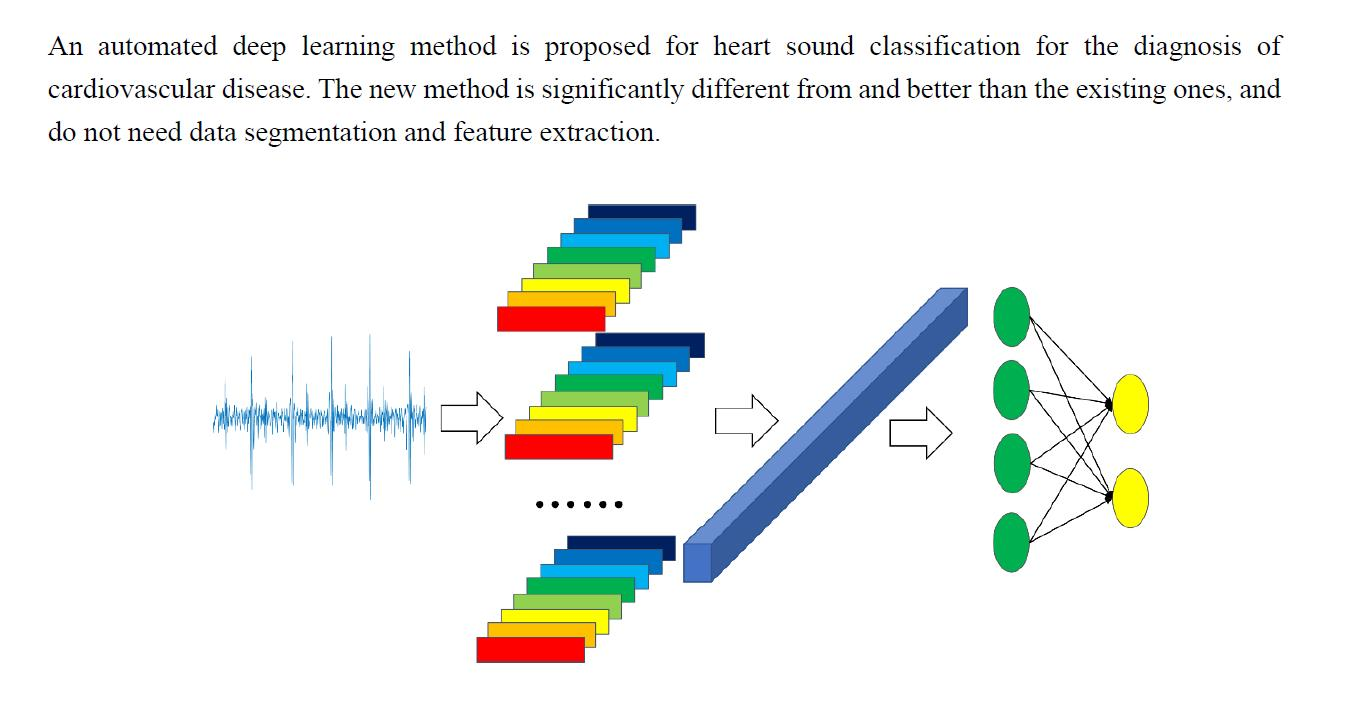
Abstract
:
1. Introduction
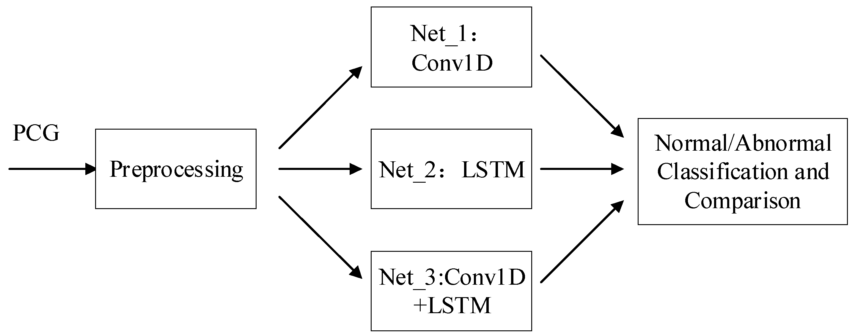
2. Materials and Methods
2.1. Dataset
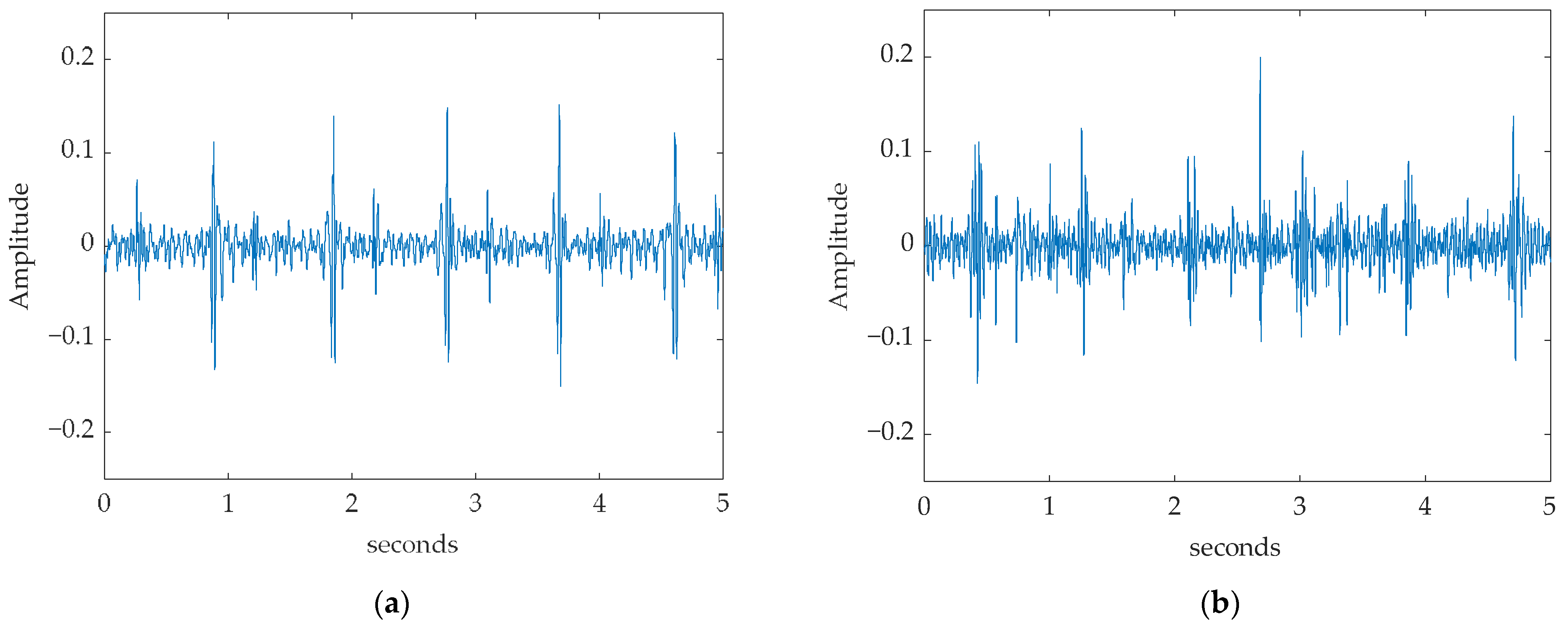
2.2. Preprocessing
2.3. Model
2.3.1. Input Layer
2.3.2. 1D-Convolutional Neural Network
2.3.3. Pooling Layers
2.3.4. Long Short-Term Memory Network
2.3.5. Dense Layers
2.3.6. Dropout Layers
2.4. Class Weight
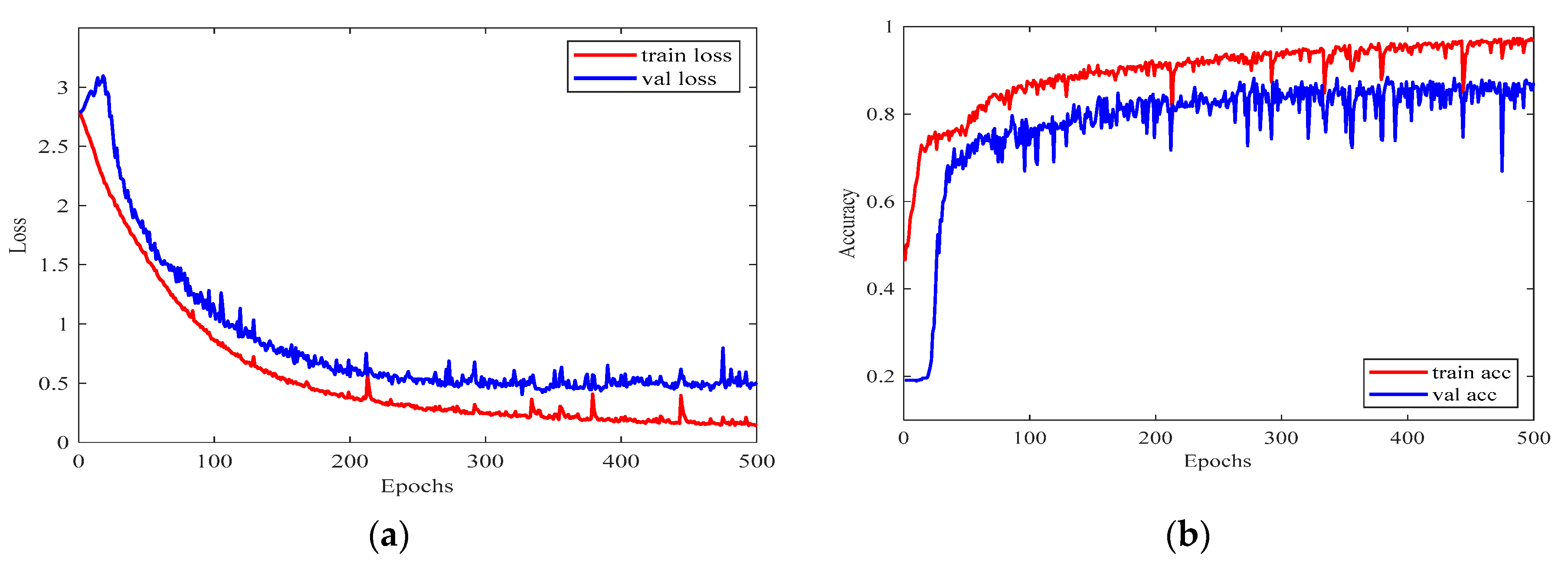
2.5. Training and Validation
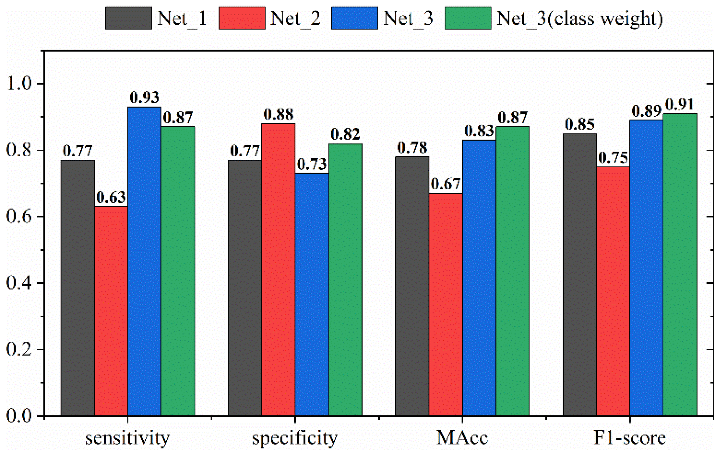
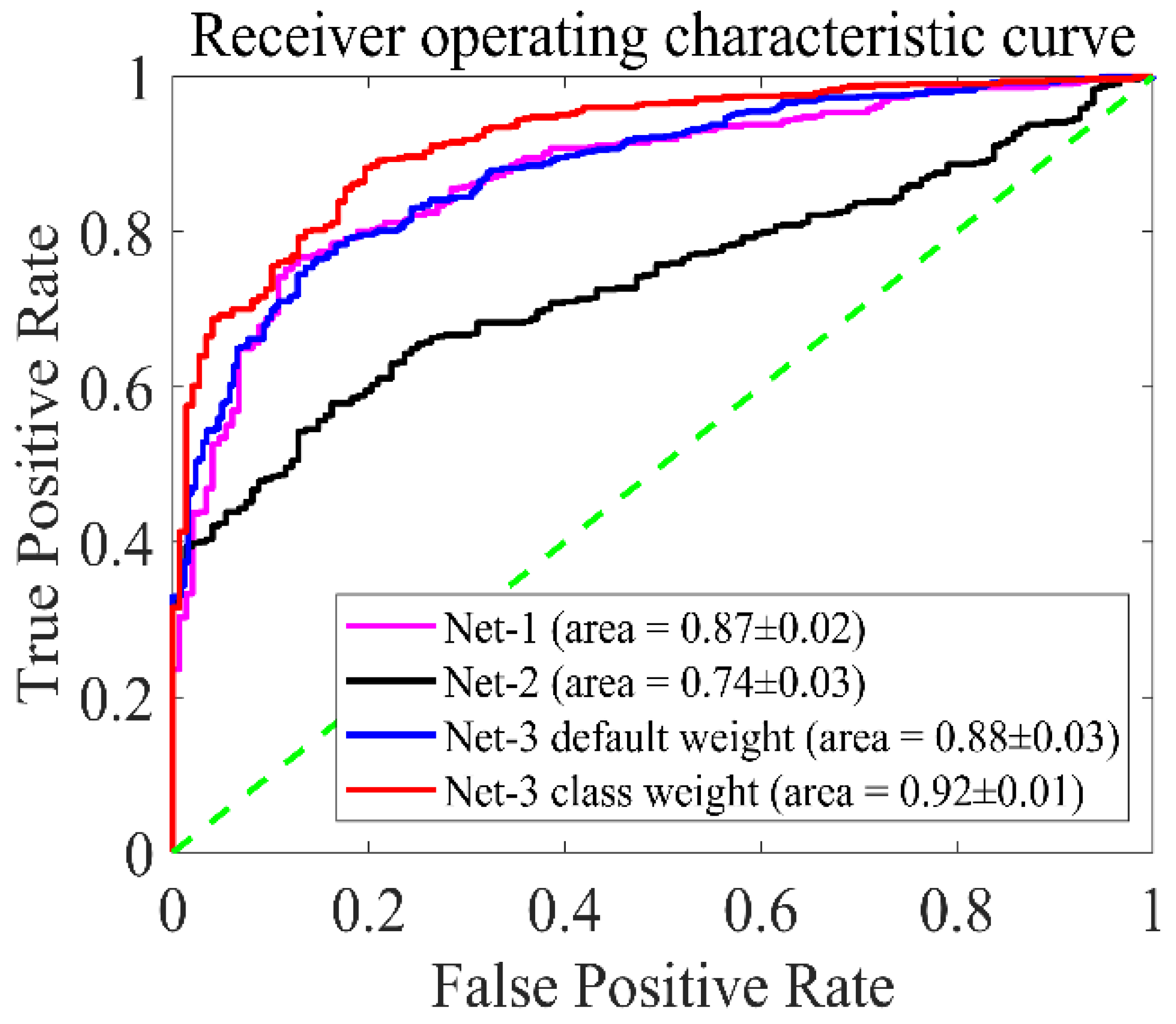
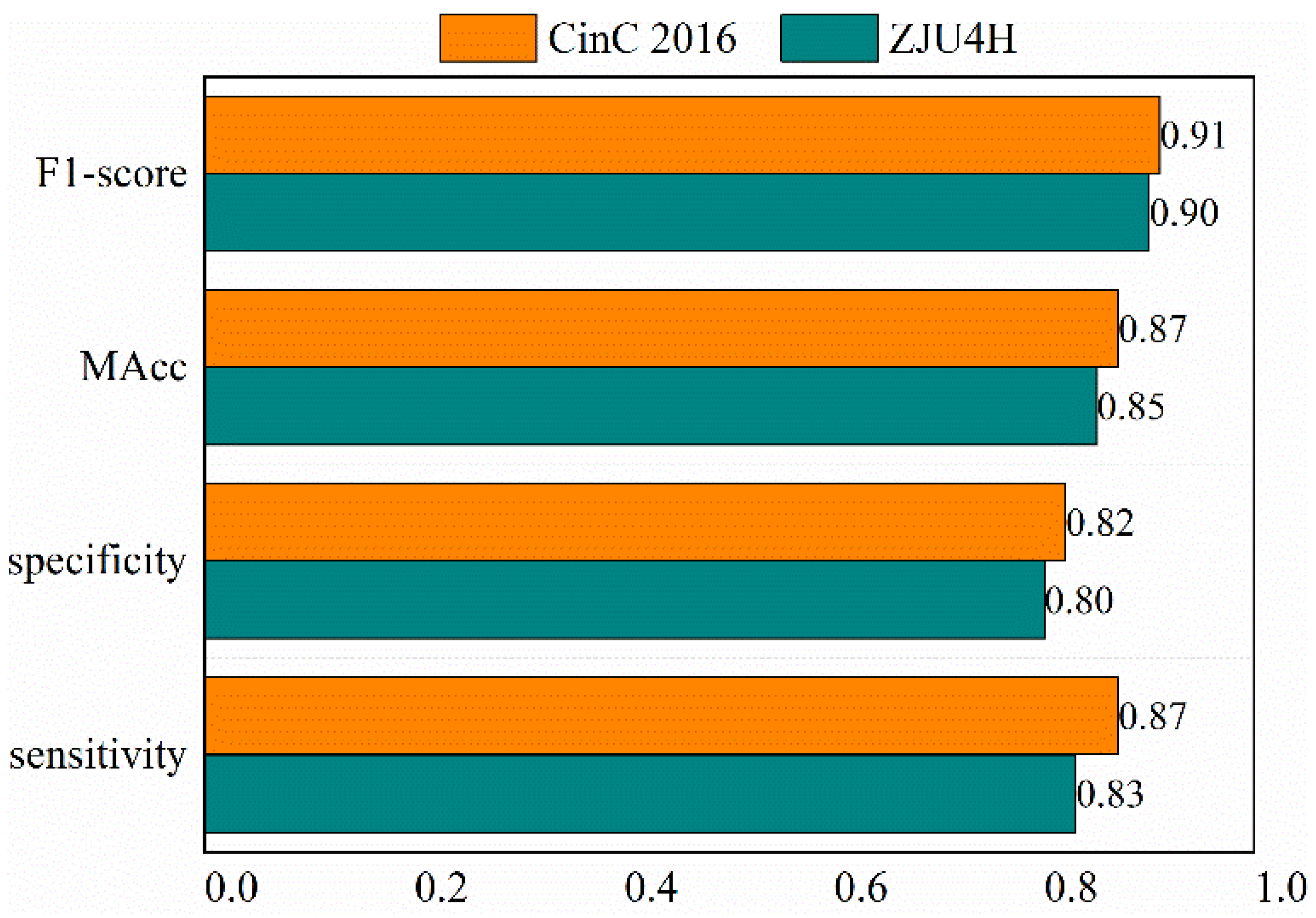
3. Results
4. Discussion
5. Conclusions
Author Contributions
Funding
Data Availability Statement
Conflicts of Interest
References
- Cardiovascular Diseases (CVDs). Available online: https://www.who.int/en/news-room/fact-sheets/detail/cardiovascular-diseases-(cvds) (accessed on 3 August 2020).
- Luisada, A.A.; Liu, C.K.; Aravanis, C.; Testelli, M.; Morris, J. On the mechanism of production of heart sounds. Am. Heart J. 1958, 55, 383–399. [Google Scholar] [CrossRef]
- Goda, M.A.; Hajas, P. Morphological Determination of Pathological PCG Signals by Time and Frequency Domain Analysis. In Proceedings of the 2016 Computing in Cardiology Conference, Vancouver, BC, Canada, 11–14 September 2016. [Google Scholar]
- Langley, P.; Murray, A. Abnormal Heart Sounds Detected from Short Duration Unsegmented Phonocardiograms by Wavelet Entropy. In Proceedings of the 2016 Computing in Cardiology Conference, Vancouver, BC, Canada, 11–14 September 2016. [Google Scholar]
- Rubin, J.; Abreu, R.; Ganguli, A.; Nelaturi, S.; Matei, I.; Sricharan, K. Classifying heart sound recordings using deep convolutional neural networks and mel-frequency cepstral coefficients. In Proceedings of the 2016 Computing in Cardiology Conference (CinC), Vancouver, BC, Canada, 11–14 September 2016. [Google Scholar]
- Singh-Miller, N.; Singh-Miller, N. Using Spectral Acoustic Features to Identify Abnormal Heart Sounds. In Proceedings of the 2016 Computing in Cardiology Conference, Vancouver, BC, Canada, 11–14 September 2016. [Google Scholar]
- Zhang, X.; Liang, Y.; Zhou, J.; Zang, Y. A novel bearing fault diagnosis model integrated permutation entropy, ensemble empirical mode decomposition and optimized SVM. Measurement 2015, 69, 164–179. [Google Scholar] [CrossRef]
- Plesinger, F.; Viscor, I.; Halamek, J.; Jurco, J.; Jurak, P. Heart sounds analysis using probability assessment. Physiol. Meas. 2017, 38, 1685–1700. [Google Scholar] [CrossRef]
- Zhang, W.; Han, J.; Deng, S.-W. Heart sound classification based on scaled spectrogram and partial least squares regression. Biomed. Signal Process. Control 2017, 32, 20–28. [Google Scholar] [CrossRef]
- Durand, L.G.; Blanchard, M. Comparison of pattern recognition methods for computer-assisted classification of spectra of heart sounds in patients with a porcine bioprosthetic valve implanted in the mitral position. IEEE Trans. Biomed. Eng. 1990, 37, 1121–1129. [Google Scholar] [CrossRef]
- Uğuz, H. A biomedical system based on artificial neural network and principal component analysis for diagnosis of the heart valve diseases. J. Med. Syst. 2012, 36, 61–72. [Google Scholar] [CrossRef]
- Oelmez, T.; Dokur, Z. Classification of Heart Sounds Using Artificial Neural Network. Pattern Recognit. Lett. 2003, 24, 617–629. [Google Scholar] [CrossRef]
- Dokur, Z.; Ölmez, T. Heart sound classification using wavelet transform and incremental self-organizing map. Digit. Signal Process. 2008, 18, 951–959. [Google Scholar] [CrossRef]
- Ari, S.; Hembram, K.; Saha, G. Detection of cardiac abnormality from PCG signal using LMS based least square SVM classifier. Expert Syst. Appl. 2010, 37, 8019–8026. [Google Scholar] [CrossRef]
- Avendao-Valencia, L.D.; Godino-Llorente, J.I.; Blanco-Velasco, M.; Castellanos-Dominguez, G. Feature extraction from parametric time-frequency representations for heart murmur detection. Ann. Biomed. Eng. 2010, 38, 2716–2732. [Google Scholar] [CrossRef]
- Quiceno-Manrique, A.F.; Godino-Llorente, J.I.; Blanco-Velasco, M.; Castellanos-Dominguez, G. Selection of Dynamic Features Based on Time–Frequency Representations for Heart Murmur Detection from Phonocardiographic Signals. Ann. Biomed. Eng. 2010, 38, 118–137. [Google Scholar] [CrossRef] [PubMed]
- Gerbarg, D.S.; Taranta, A.; Spagnuolo, M.; Hofler, J. Computer analysis of phonocardiograms. Prog. Cardiovasc. Dis. 1963, 5, 393–405. [Google Scholar] [CrossRef]
- Springer, D.B.; Tarassenko, L.; Clifford, G.D. Logistic Regression-HSMM-Based Heart Sound Segmentation. IEEE Trans. Biomed. Eng. 2016, 63, 822–832. [Google Scholar] [CrossRef] [PubMed]
- Hong, T.; Ziyin, D.; Yuanlin, J.; Ting, L.; Chengyu, L. PCG Classification Using Multidomain Features and SVM Classifier. BioMed Res. Int. 2018, 2018, 4205027. [Google Scholar]
- Krishnan, P.; Balasubramanian, P.; Umapathy, S. Automated heart sound classification system from unsegmented phonocardiogram (PCG) using deep neural network. Phys. Eng. Sci. Med. 2020, 43, 505–515. [Google Scholar] [CrossRef]
- Liu, C.; Springer, D.; Li, Q.; Moody, B.; Juan, R.A.; Chorro, F.J.; Castells, F.; Roig, J.M.; Silva, I.; Johnson, A.E.W. An open access database for the evaluation of heart sound algorithms. Physiol. Meas. 2016, 37, 2181–2213. [Google Scholar] [CrossRef]
- Goldberger, A.; Luis, M.; Amaral, N.; Glass, P.; Jeffrey, P.; Hausdorff, J.; Peng, C.-K.; Stanley, H. PhysioBank, PhysioToolkit, and PhysioNet. Circulation 2000, 101, E215–E220. [Google Scholar] [CrossRef] [Green Version]
- Karim, F.; Majumdar, S.; Darabi, H.; Chen, S. LSTM Fully Convolutional Networks for Time Series Classification. IEEE Access 2018, 6, 1662–1669. [Google Scholar] [CrossRef]
- Ruder, S. An overview of gradient descent optimization algorithms. arXiv 2016, arXiv:1609.04747. [Google Scholar]
- Homsi, M.N.; Warrick, P. Ensemble methods with outliers for phonocardiogram classification. Physiol. Meas. 2017, 38, 1631–1644. [Google Scholar] [CrossRef]
- Li, F.; Tang, H.; Shang, S.; Mathiak, K.; Cong, F. Classification of Heart Sounds Using Convolutional Neural Network. Appl. Sci. 2020, 10, 3956. [Google Scholar] [CrossRef]


| Dataset | Number of PCG | Normal PCG | Abnormal PCG | Training Datasets | Validation Datasets | Test Datasets |
|---|---|---|---|---|---|---|
| Dataset-a | 409 | 117 | 292 | 245 | 82 | 82 |
| Dataset-b | 490 | 370 | 102 | 294 | 98 | 98 |
| Dataset-c | 31 | 7 | 24 | 19 | 6 | 6 |
| Dataset-d | 55 | 21 | 28 | 33 | 11 | 11 |
| Dataset-e | 2000 | 1876 | 124 | 1200 | 400 | 400 |
| Dataset-f | 114 | 76 | 34 | 68 | 23 | 23 |
| Total Cinc | 3099 | 2483 | 616 | 1859 | 620 | 620 |
| Layer (Type) | Params |
|---|---|
| Input | [1 × 10,000] PCG time sequence |
| Conv1D | Filters = 64, 1 × 100, ReLU Filters = 32, 1 × 100, ReLU Filters = 32, 1 × 100, ReLU |
| Dropout | dropout rate = 0.5 |
| MaxPooling1D | Pool size = 2, strides = 2 |
| Flatten | |
| Dropout | dropout rate = 0.3 |
| Dense | 1 × 512, ReLU 1 × 128, ReLU 1 × 64, ReLU |
| Output | 1 × 2, Softmax |
| Layer (Type) | Params |
|---|---|
| Input | [1 × 10,000] PCG time sequence |
| LSTM | Units = 512 Units = 256 Units = 128 |
| Dropout | dropout rate = 0.5 |
| Dense | 1 × 64, ReLU |
| Output | 1 × 2, Softmax |
| Layer (Type) | Params |
|---|---|
| Input | [1 × 100 × 100] PCG time sequence |
| Time Distributed Conv1D | Filters = 8, 1 × 5, ReLU Filters = 4, 1 × 5, ReLU Filters = 2, 1 × 1, ReLU |
| Dropout | dropout rate = 0.5 |
| Time Distributed MaxPooling1D | Pool size = 2, strides = 2 |
| Time Distributed Flatten | |
| LSTM | Units = 256 |
| Dense | 1 × 128, ReLU |
| Dropout | dropout rate = 0.3 |
| Output | 1 × 2, Softmax |
| Related Work | Method | Performance | |
|---|---|---|---|
| Masun et al. [25] | Random forest + LogitBoost + Cost-sensitive classifier | Sensitivity: Specificity: MAcc: | 80% 81% 80% |
| Li et al. [26] | CNN | Sensitivity: Specificity: MAcc: | 87% 86% 86% |
| Krishnan et al. [20] | DNN | Sensitivity: Specificity: MAcc: F1-score: AUC: | 87% 85% 86% 85% 86% |
| This study (Net_3 with class weight) | 1D-CNN + LSTM | Sensitivity: Specificity: MAcc: F1-score: AUC: | 87% 82% 86% 91% 92% |
Publisher’s Note: MDPI stays neutral with regard to jurisdictional claims in published maps and institutional affiliations. |
© 2022 by the authors. Licensee MDPI, Basel, Switzerland. This article is an open access article distributed under the terms and conditions of the Creative Commons Attribution (CC BY) license (https://creativecommons.org/licenses/by/4.0/).
Share and Cite
Chen, D.; Xuan, W.; Gu, Y.; Liu, F.; Chen, J.; Xia, S.; Jin, H.; Dong, S.; Luo, J. Automatic Classification of Normal–Abnormal Heart Sounds Using Convolution Neural Network and Long-Short Term Memory. Electronics 2022, 11, 1246. https://doi.org/10.3390/electronics11081246
Chen D, Xuan W, Gu Y, Liu F, Chen J, Xia S, Jin H, Dong S, Luo J. Automatic Classification of Normal–Abnormal Heart Sounds Using Convolution Neural Network and Long-Short Term Memory. Electronics. 2022; 11(8):1246. https://doi.org/10.3390/electronics11081246
Chicago/Turabian StyleChen, Ding, Weipeng Xuan, Yexing Gu, Fuhai Liu, Jinkai Chen, Shudong Xia, Hao Jin, Shurong Dong, and Jikui Luo. 2022. "Automatic Classification of Normal–Abnormal Heart Sounds Using Convolution Neural Network and Long-Short Term Memory" Electronics 11, no. 8: 1246. https://doi.org/10.3390/electronics11081246