
Detail Enhancement Multi-Exposure Image Fusion Based on Homomorphic Filtering

Abstract
:1. Introduction
- This paper applies homomorphic filtering to the multi-exposure image fusion algorithm for the first time. Other detail enhancement algorithms will lose some low-frequency signals when enhancing high-frequency details, while homomorphic filtering can enhance details while retaining low-frequency signals and can enhance the details based on retaining the original image information.
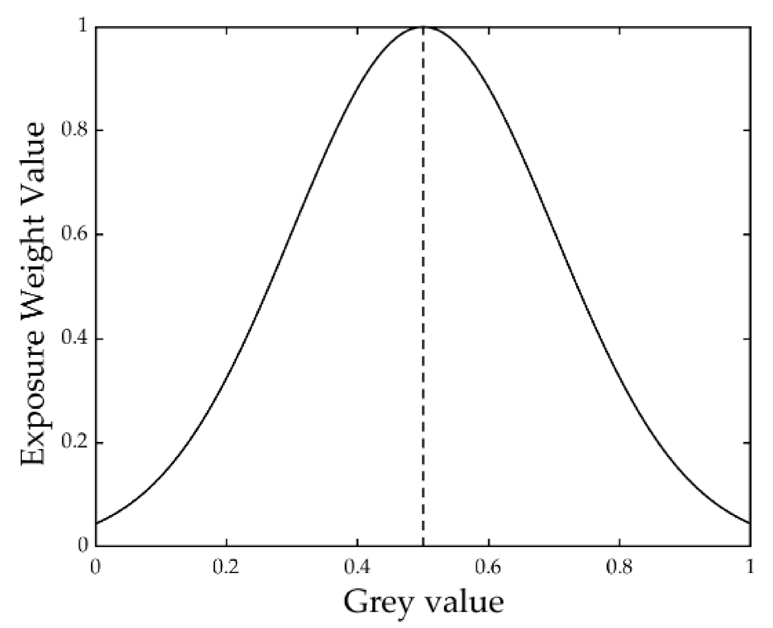
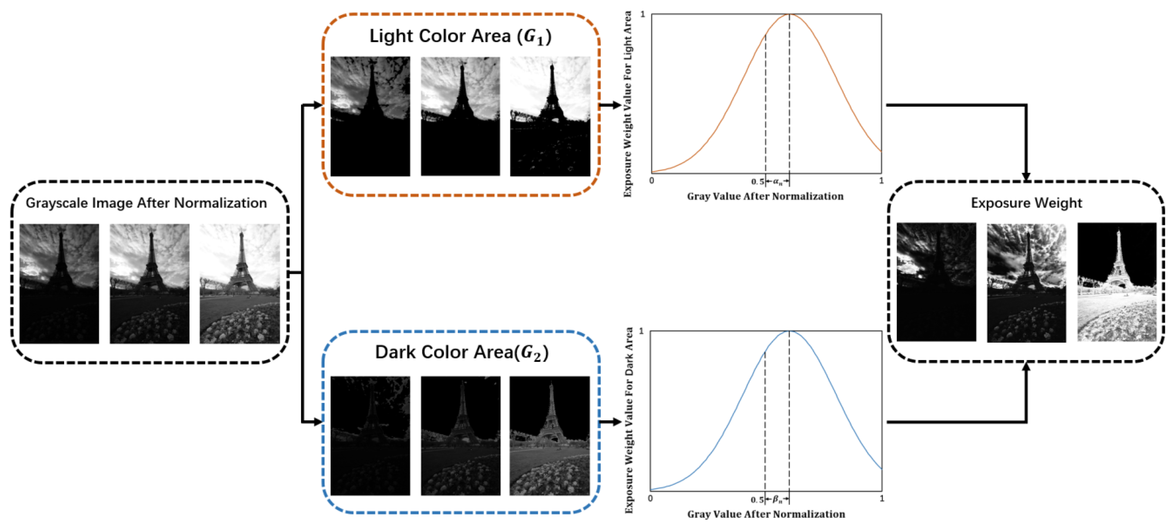
- An exposure weighting algorithm based on threshold segmentation and adaptively adjustable Gaussian curve is proposed, which assigns more reasonable weights to well-exposed areas and retains more detailed information.
- The Laplacian pyramid is improved based on homomorphic filtering, which enhances the edge details of the fused image and generates an image with obvious details.
2. Related Works
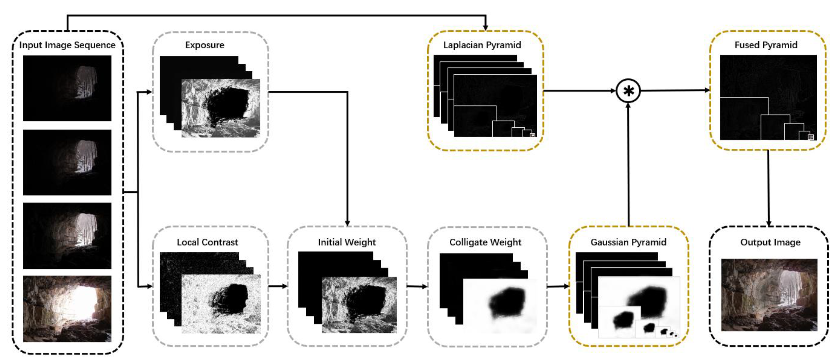
3. Proposed Method
| Algorithm 1: The proposed algorithm. |
| Parameter: represents the grayscale image of , means normalized to , Input: Source image sequences Output: The result after fusion |
| 1: for each image do |
| 2: Calculate by Equation (3) |
| 3: while Equation (4) do |
| 4: |
| 5: Calculate by Equation (3) |
| 6: end while |
| 7: The optimal threshold of the th image |
| 8: end for |
| 9: for each image do |
| 10: Calculate and separately by Equations (5) and (6) |
| 11: Use Equations (7) and (8) to assign weights to |
| 12: end for |
| 13: for each image do |
| 14: the local contrast value is calculated by Equation (9) |
| 15: Use Equation (11) to assign weights to |
| 16: end for |
| 17: Use Equation (12) to calculate the initial weight map |
| 18: Use Equation (13) to denoise , and get after normalization |
| 19: Use Equations (14)–(16) to calculate |
| 20: Reconstructed pyramid fused into by Equations (17)–(19) |
3.1. Exposure Weight
3.2. Local Contrast Weight
3.3. Pyramid Fusion Based on Homomorphic Filter Detail Enhancement
| Algorithm 2: Homomorphic filtering algorithm. |
| Parameter: Input: Laplacian pyramid of the source image Output: Laplacian pyramid with enhanced detail |
| 1: for each layer of do |
| 2: |
| 3: The Fourier transform |
| 4: |
| 5: |
| 6: Filtering the Fourier transform |
| 7: Inverse the Fourier transform |
| 8: Indexation |
| 9: Take the real part to get the enhanced pyramid |
| 10: end for |
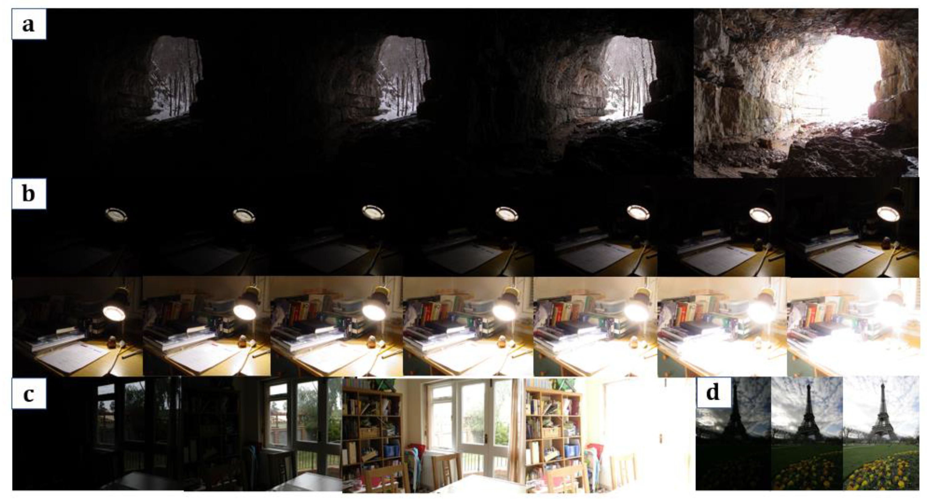
4. Experimental Results and Analysis
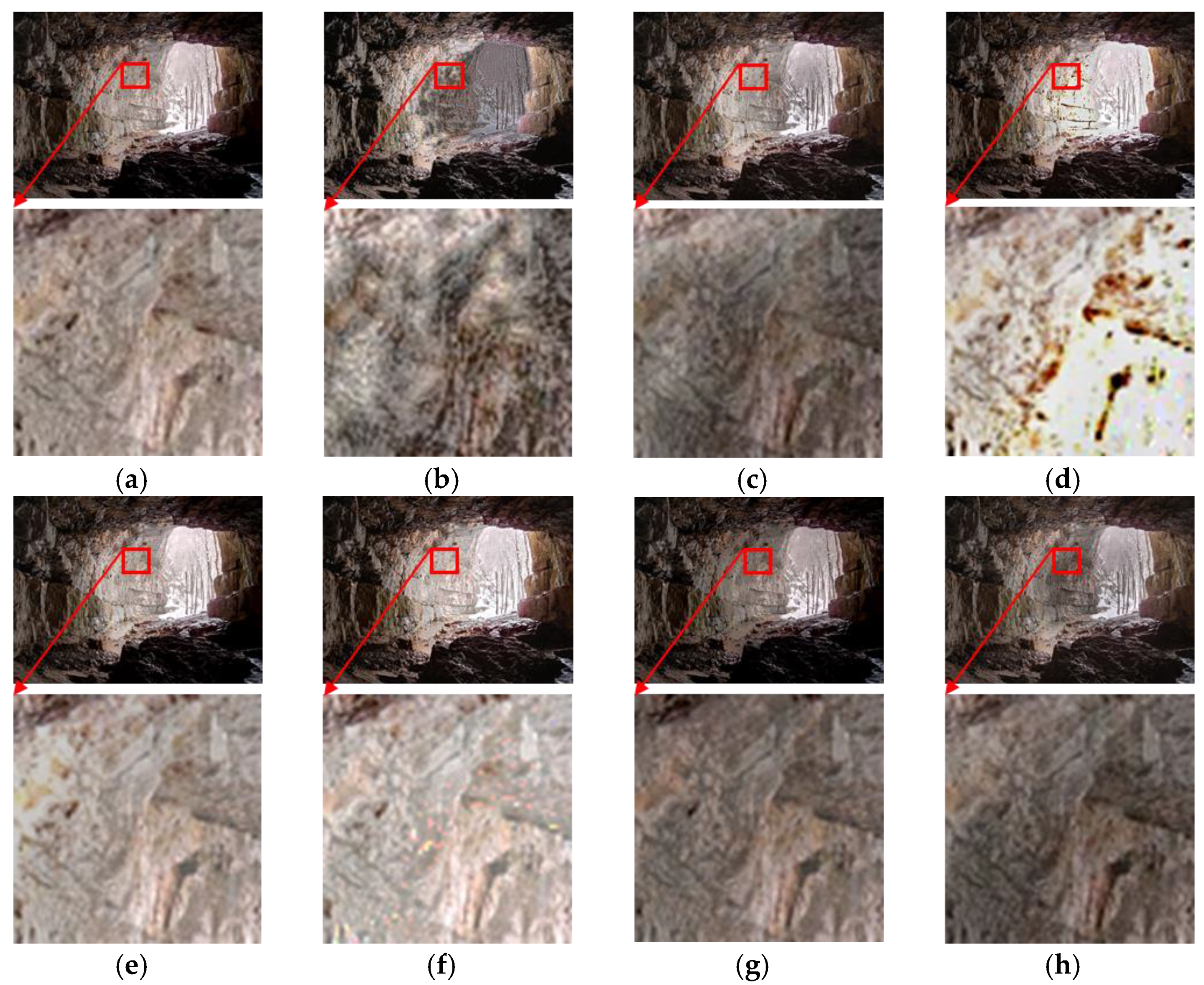
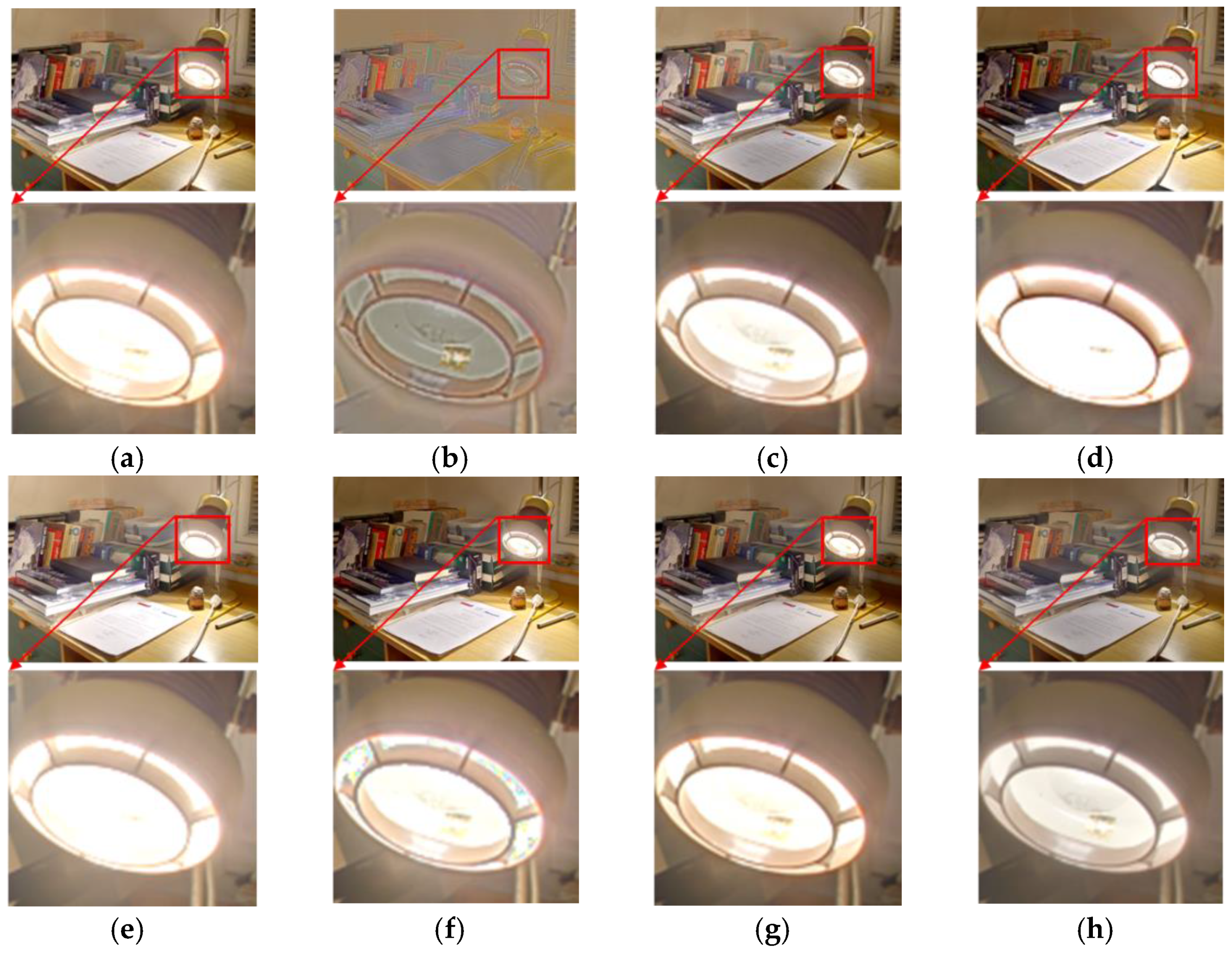
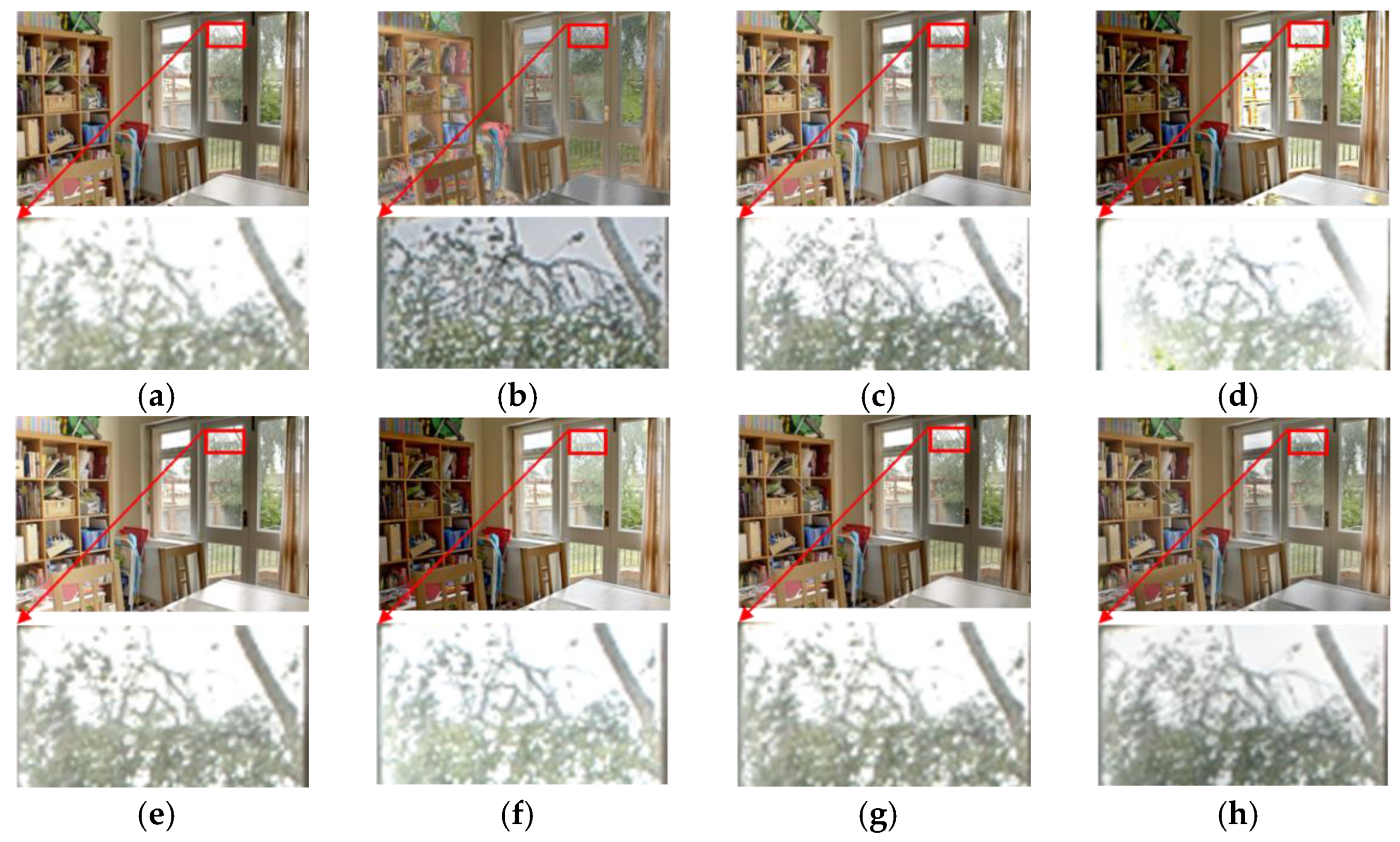
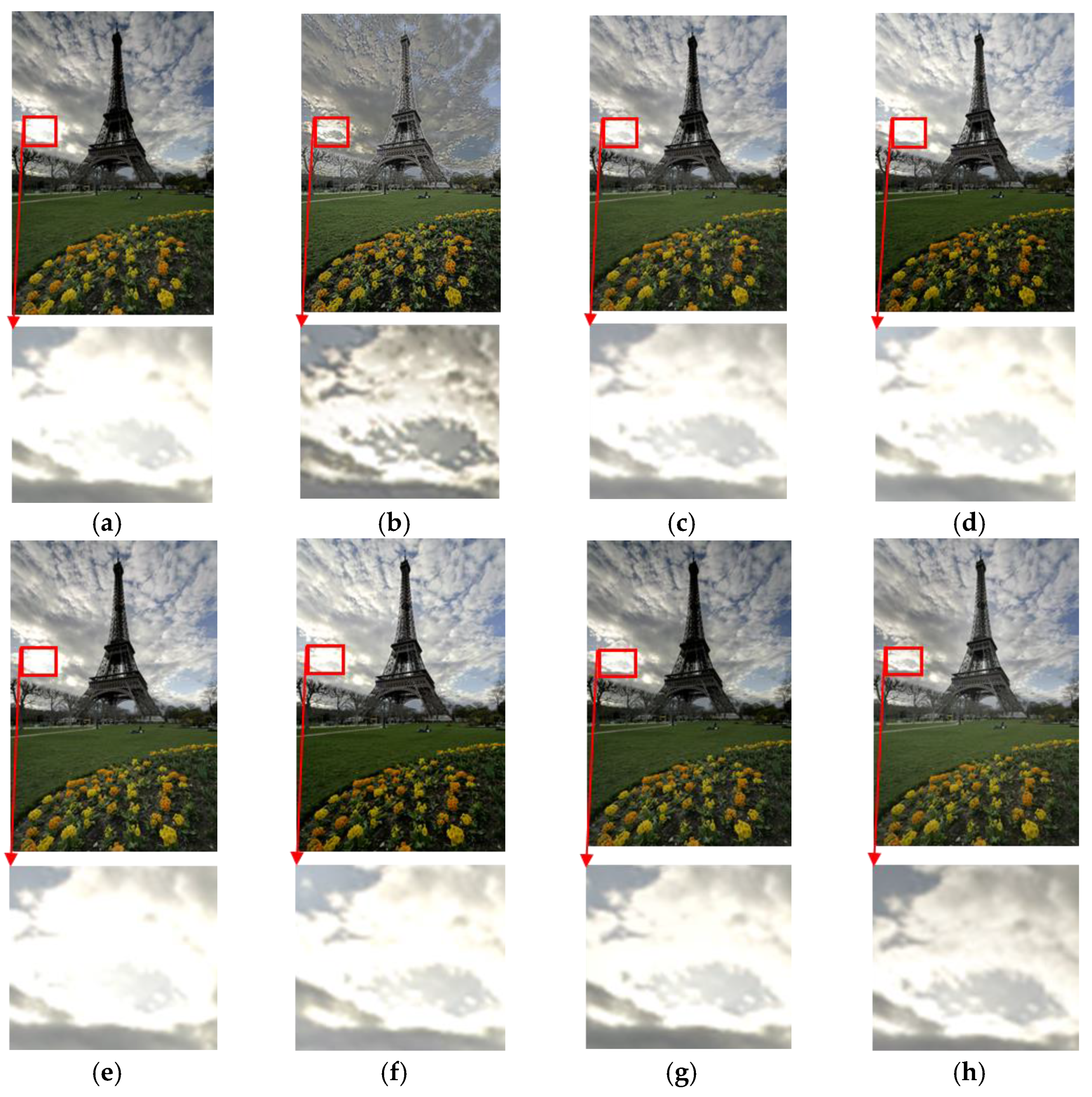
4.1. Subjective Analysis
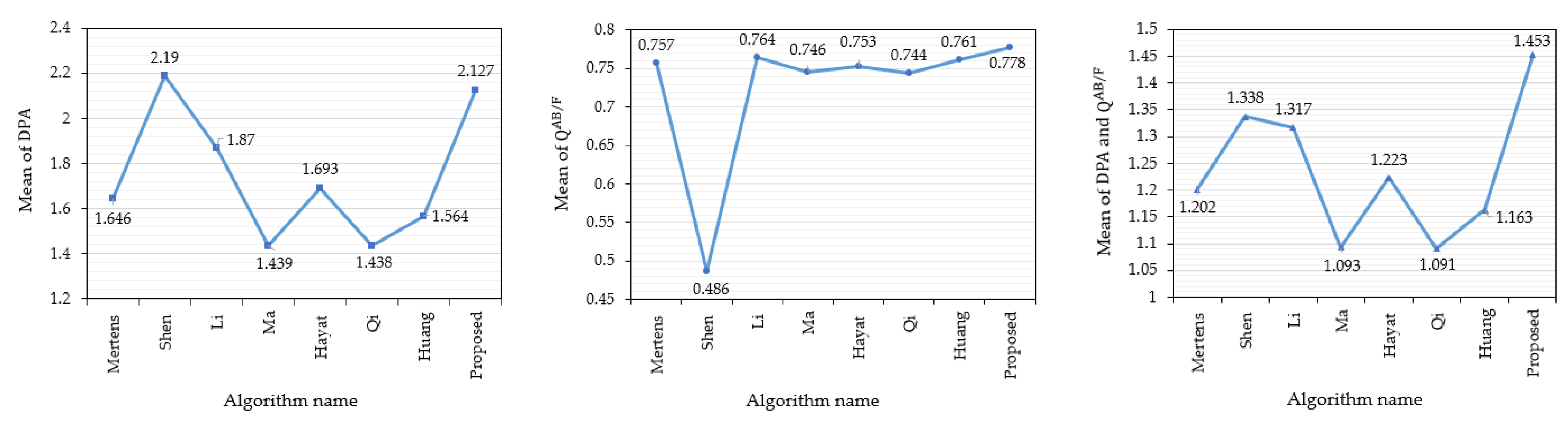
4.2. Objective Evaluation
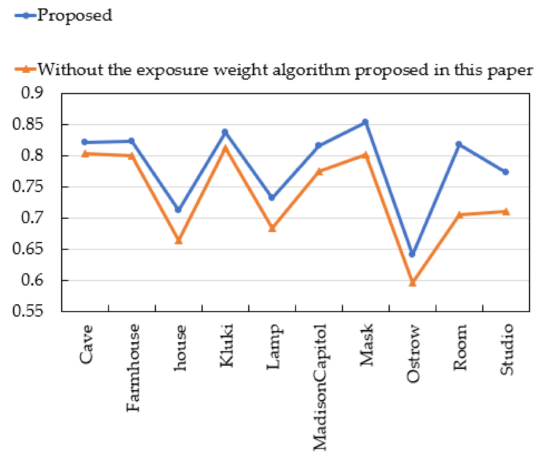
4.3. The Comparative Experiment of Adaptive Exposure Weight Calculation
5. Conclusions
Author Contributions
Funding
Acknowledgments
Conflicts of Interest
References
- Akçay, Ö.; Erenoğlu, R.C.; Avşar, E.Ö. The effect of JPEG compression in close range photogrammetry. Int. J. Eng. Geosci. 2017, 2, 35–40. [Google Scholar] [CrossRef] [Green Version]
- Chaurasiya, R.K.; Ramakrishnan, K. High dynamic range imaging. In Proceedings of the 2013 International Conference on Communication Systems and Network Technologies, Gwalior, India, 6–8 April 2013; pp. 83–89. [Google Scholar]
- Wang, S.; Zhao, Y. A Novel Patch-Based Multi-Exposure Image Fusion Using Super-Pixel Segmentation. IEEE Access 2020, 8, 39034–39045. [Google Scholar] [CrossRef]
- Shao, H.; Jiang, G.; Yu, M.; Song, Y.; Jiang, H.; Peng, Z.; Chen, F. Halo-Free Multi-Exposure Image Fusion Based on Sparse Representation of Gradient Features. Appl. Sci. 2018, 8, 1543. [Google Scholar] [CrossRef] [Green Version]
- Li, Z.; Zheng, J. Visual-Salience-Based Tone Mapping for High Dynamic Range Images. IEEE Trans. Ind. Electron. 2014, 61, 7076–7082. [Google Scholar] [CrossRef]
- Yilmaz, I.; Bildirici, I.O.; Yakar, M.; Yildiz, F. Color calibration of scanners using polynomial transformation. In Proceedings of the XXth ISPRS Congress Commission V, Istanbul, Turkey, 12–23 July 2004; pp. 890–896. [Google Scholar]
- Grossberg, M.D.; Nayar, S.K. Determining the Camera Response from Images: What Is Knowable? IEEE Trans. Pattern Anal. Mach. Intell. 2003, 25, 1455–1467. [Google Scholar] [CrossRef] [Green Version]
- Kou, F.; Li, Z.; Wen, C.; Chen, W. Edge-preserving smoothing pyramid based multi-scale exposure fusion. J. Vis. Commun. Image Represent. 2018, 53, 235–244. [Google Scholar] [CrossRef]
- Sağlam, A.; Baykan, N.A. A new color distance measure formulated from the cooperation of the Euclidean and the vector angular differences for lidar point cloud segmentation. Int. J. Eng. Geosci. 2021, 6, 117–124. [Google Scholar] [CrossRef]
- Gu, B.; Li, W.; Wong, J.; Zhu, M.; Wang, M. Gradient field multi-exposure images fusion for high dynamic range image visualization. J. Vis. Commun. Image Represent. 2012, 23, 604–610. [Google Scholar] [CrossRef]
- Li, S.T.; Kang, X.D. Fast Multi-exposure Image Fusion with Median Filter and Recursive Filter. IEEE Trans. Consum. Electron. 2012, 58, 626–632. [Google Scholar] [CrossRef] [Green Version]
- Huang, F.; Zhou, D.; Nie, R.; Yu, C. A color multi-exposure image fusion approach using structural patch decomposition. IEEE Access 2018, 6, 42877–42885. [Google Scholar] [CrossRef]
- Meher, B.; Agrawal, S.; Panda, R.; Abraham, A. A survey on region based image fusion methods. Inf. Fusion 2018, 48. [Google Scholar] [CrossRef]
- Burt, P.J.; Adelson, E.H. A multiresolution spline with application to image mosaics. ACM Trans. Graph. 1983, 2, 217–236. [Google Scholar] [CrossRef]
- Singh, S.; Mittal, N.; Singh, H. Review of Various Image Fusion Algorithms and Image Fusion Performance Metric. Arch. Comput. Methods Eng. 2021, 28, 3645–3659. [Google Scholar] [CrossRef]
- Mertens, T.; Kautz, J.; van Reeth, F. Exposure Fusion: A Simple and Practical Alternative to High Dynamic Range Photography. Comput. Graph. Forum 2009, 28, 161–171. [Google Scholar] [CrossRef]
- Wang, C.M.; He, C.; Xu, M.F. Fast exposure fusion of detail enhancement for brightest and darkest regions. Vis. Comput. 2021, 37, 1233–1243. [Google Scholar] [CrossRef]
- Xu, H.; Ma, J.; Zhang, X.-P. MEF-GAN: Multi-Exposure Image Fusion via Generative Adversarial Networks. IEEE Trans. Image Process. 2020, 29, 7203–7216. [Google Scholar] [CrossRef]
- Yang, Y.; Wu, J.H.; Huang, S.Y.; Lin, P. Multiexposure Estimation and Fusion Based on a Sparsity Exposure Dictionary. IEEE Trans. Instrum. Meas. 2020, 69, 4753–4767. [Google Scholar] [CrossRef]
- Ulucan, O.; Karakaya, D.; Turkan, M. Multi-exposure image fusion based on linear embeddings and watershed masking. Signal Process. 2021, 178. [Google Scholar] [CrossRef]
- Shen, J.; Zhao, Y.; Yan, S.; Li, X. Exposure fusion using boosting Laplacian pyramid. IEEE Trans Cybern 2014, 44, 1579–1590. [Google Scholar] [CrossRef]
- Li, Z.; Wei, Z.; Wen, C.; Zheng, J. Detail-Enhanced Multi-Scale Exposure Fusion. IEEE Trans Image Process. 2017, 26, 1243–1252. [Google Scholar] [CrossRef]
- Li, Z.; Zheng, J.; Zhu, Z.; Yao, W.; Wu, S. Weighted Guided Image Filtering. IEEE Trans. Image Process. 2014, 24, 120–129. [Google Scholar] [CrossRef]
- Kede, M.; Hui, L.; Hongwei, Y.; Zhou, W.; Deyu, M.; Lei, Z. Robust Multi-Exposure Image Fusion: A Structural Patch Decomposition Approach. IEEE Trans Image Process. 2017, 26, 2519–2532. [Google Scholar] [CrossRef]
- Hayat, N.; Imran, M. Ghost-free multi exposure image fusion technique using dense SIFT descriptor and guided filter. J. Vis. Commun. Image Represent. 2019, 62, 295–308. [Google Scholar] [CrossRef]
- Liu, Y.; Wang, Z. Dense SIFT for ghost-free multi-exposure fusion. J. Vis. Commun. Image Represent. 2015, 31, 208–224. [Google Scholar] [CrossRef]
- Qi, G.; Chang, L.; Luo, Y.; Chen, Y.; Zhu, Z.; Wang, S. A Precise Multi-Exposure Image Fusion Method Based on Low-level Features. Sensors 2020, 20, 1597. [Google Scholar] [CrossRef] [PubMed] [Green Version]
- Huang, L.; Li, Z.; Xu, C.; Feng, B. Multi-exposure image fusion based on feature evaluation with adaptive factor. IET Image Process. 2021, 15, 3211–3220. [Google Scholar] [CrossRef]
- Agrawal, A.; Raskar, R.; Nayar, S.K.; Li, Y.Z. Removing photography artifacts using gradient projection and flash-exposure sampling. Acm Trans. Graph. 2005, 24, 828–835. [Google Scholar] [CrossRef]
- Chen, Y.B.; Chen, O.T.C. Image Segmentation Method Using Thresholds Automatically Determined from Picture Contents. EURASIP J. Image Video Process. 2009, 2009, 140492. [Google Scholar] [CrossRef] [Green Version]
- Yugander, P.; Tejaswini, C.H.; Meenakshi, J.; Kumar, K.S.; Varma, B.V.N.S.; Jagannath, M. MR Image Enhancement using Adaptive Weighted Mean Filtering and Homomorphic Filtering. Procedia Comput. Sci. 2020, 167, 677–685. [Google Scholar] [CrossRef]
- Okonek, B. HDR Photography Gallery Samples. Available online: http://www.easyhdr.com/examples (accessed on 8 March 2022).
- HDR Projects Software. Available online: http://www.projects-software.com/HDR (accessed on 8 March 2022).
- Cadik, M. Martin Cadik HDR Webpage. Available online: http://cadik.posvete.cz/tmo (accessed on 9 March 2022).
- HDRsoft Gallery. Available online: http://www.hdrsoft.com/gallery (accessed on 7 March 2022).
- Verma, C.S. Chaman Singh Verma HDR Webpage. Available online: http://pages.cs.wisc.edu//CS766_09/HDRI/hdr.html (accessed on 7 March 2022).
- HDR Pangeasoft. Available online: http://pangeasoft.net/pano/bracketeer/ (accessed on 7 March 2022).
- Hvdwolf. Enfuse HDR Webpage. Available online: http://www.photographers-toolbox.com/products/lrenfuse.php (accessed on 11 March 2022).
- Keerativittayanun, S.; Kondo, T.; Kotani, K.; Phatrapornnant, T.; Karnjana, J. Two-layer pyramid-based blending method for exposure fusion. Mach. Vis. Appl. 2021, 32, 1–18. [Google Scholar] [CrossRef]
- Xydeas, C.; Petrovic, V. Objective image fusion performance measure. Electron. Lett. 2000, 36, 308–309. [Google Scholar] [CrossRef] [Green Version]


| Algorithm | Method | Application | Dataset | Result |
|---|---|---|---|---|
| Mertens [16] | Contrast, saturation, and well-exposedness are proposed to construct a fused image weight map, fused using Laplacian pyramids. | MATLAB | 15 static images by Jacques Joffre, Jesse Levinson, Agrawal [29] and themselves | Subjective comparison test with three algorithms |
| Shen [21] | Using local weights, global weights, and JND-based saliency weights to estimate exposure weight maps for enhancing detail and base signals of Laplacian pyramids. | MATLAB | 18 static images by themselves | Subjective comparison test with five algorithms |
| Li [22] | The image details are extracted with the weighted structure tensor, the Gaussian pyramid of the luminance component of the source image sequence is used as the guide image, the weighted smoothing is applied to all the weighted Gaussian pyramids, and finally the multi-resolution fusion is performed. | MATLAB | 6 static images by Laurance Meylan, Dani Lischinski, Jacques Joffre, Martin Cadik, Erik Reinhard, and themselves | Subjective and comparative testing of three algorithms |
| Ma [24] | It is proposed to decompose the image into three components: signal intensity, signal structure, and average intensity fuse each component separately and finally reconstruct a fused image. | MATLAB | 21 static scenes and 19 dynamic scenes by Bartlomiej Okonek, Erik Reinhard, Dani Lischinski, Jianbing Shen, Mertens, Orazio Gallo et al. | Subjective comparison with 12 algorithms, Compare with nine algorithms in the static scenario, computational complexity comparison with seven algorithms, average execution time comparison with six algorithms |
| Hayat [25] | The local contrast, brightness, and color dissimilar features are proposed to estimate the initial weights, where the local contrast is calculated by DSIFT, and pyramid fusion is used after denoising by a guided filter. | MATLAB | 8 images by Mertens, Jianbing Shen et al. | Subjective, , , and comparative testing of three algorithms |
| Qi [27] | The source image is decomposed into a base layer and a detail layer with a guided filter, the base layer is calculated based on image blocks, and the detail layer is weighted according to the local average brightness change. | MATLAB | 24 static scenes and 15 dynamic scenes by Ma, Hu, and Sen | The subjectivity of the six algorithms and their mean values , , and are compared |
| Huang [28] | Based on the Mertens method, the adaptive factor exposure evaluation weight is proposed, the Sobel operator is used to calculate the texture change weight, and finally, the pyramid is fused. | MATLAB | 20 static images by Ma | Subjective, , and comparative testing of eight algorithms |
| Proposed | Based on the Mertens method, the exposure weight calculated by threshold segmentation and adaptively adjustable Gaussian curve is proposed, and the detail layer of the Laplacian pyramid is enhanced by homomorphic filtering. | MATLAB | 17 static images by Ma | Subjective, and comparative testing of seven algorithms |
| Source Sequence | Size | Image Origin |
|---|---|---|
| Arno | 339 × 512 × 3 | Bartlomiej Okonek [32] |
| Cave | 512 × 384 × 4 | Bartlomiej Okonek [32] |
| Chinese Garden | 512 × 340 × 3 | Bartlomiej Okonek [32] |
| Church | 335 × 512 × 3 | Jianbing Shen [21] |
| Farmhouse | 512 × 341 × 4 | HDR projects [33] |
| house | 512 × 340 × 4 | Mertens [16] |
| Kluki | 512 × 341 × 3 | Bartlomiej Okonek [32] |
| Lamp | 512 × 384 × 15 | Martin Cadik [34] |
| Landscape | 512 × 341 × 3 | HDRsoft [35] |
| Laurenziana | 356 × 512 × 3 | Bartlomiej Okonek [32] |
| Madison Capitol | 512 × 384 × 30 | Chaman Singh Verma [36] |
| Mask | 512 × 341 × 3 | HDRsoft [35] |
| Ostrow | 341 × 512 × 3 | Bartlomiej Okonek [32] |
| Room | 512 × 340 × 3 | Pangeasoft [37] |
| Studio | 512 × 341 × 5 | HDRsoft [35] |
| Tower | 512 × 341 × 3 | Jacques Joffre [35] |
| Window | 384 × 512 × 3 | Hvdwolf [38] |
| Images | Mertens [16] | Shen [21] | Li [22] | Ma [24] | Hayat [25] | Qi [27] | Huang [28] | Proposed |
|---|---|---|---|---|---|---|---|---|
| Arno | 1.745/0.616 | 2.105/0.369 | 1.746/0.57 | 1.476/0.593 | 1.63/0.573 | 1.462/0.579 | 1.689/0.629 | 2.296/0.622 |
| Cave | 1.735/0.795 | 2.249/0.561 | 2.26/0.834 | 1.905/0.741 | 1.797/0.801 | 1.915/0.798 | 1.716/0.719 | 2.351/0.822 |
| Chinese Garden | 1.427/0.812 | 2.173/0.475 | 1.628/0.825 | 1.135/0.826 | 1.455/0.822 | 1.095/0.812 | 1.335/0.825 | 2.07/0.831 |
| Church | 1.788/0.846 | 1.823/0.634 | 2.054/0.85 | 1.817/0.852 | 2.053/0.844 | 1.742/0.829 | 1.62/0.853 | 2.125/0.871 |
| Farmhouse | 2.572/0.8 | 2.481/0.645 | 2.544/0.809 | 2.357/0.804 | 2.622/0.804 | 2.357/0.78 | 2.39/0.804 | 2.76/0.823 |
| house | 1.172/0.693 | 1.821/0.407 | 1.422/0.698 | 1.131/0.567 | 1.296/0.685 | 1.257/0.681 | 1.152/0.707 | 1.496/0.712 |
| Kluki | 1.433/0.823 | 1.821/0.535 | 1.662/0.837 | 1.386/0.83 | 1.57/0.831 | 1.37/0.811 | 1.404/0.839 | 1.879/0.837 |
| Lamp | 1.235/0.743 | 2.797/0.378 | 1.536/0.73 | 0.892/0.724 | 1.168/0.708 | 0.869/0.721 | 1.118/0.749 | 1.417/0.731 |
| Landscape | 1.81/0.611 | 2.281/0.339 | 2.012/0.614 | 1.211/0.631 | 1.886/0.604 | 1.197/0.594 | 1.609/0.641 | 2.534/0.626 |
| Laurenziana | 1.416/0.807 | 1.905/0.572 | 1.551/0.82 | 1.12/0.814 | 1.459/0.816 | 1.053/0.799 | 1.417/0.818 | 1.989/0.826 |
| Madison Capitol | 1.02/0.817 | 2.384/0.443 | 1.082/0.819 | 0.838/0.781 | 1.046/0.787 | 0.83/0.766 | 0.964/0.822 | 1.527/0.816 |
| Mask | 1.631/0.828 | 2.443/0.496 | 2.084/0.847 | 1.28/0.841 | 1.729/0.846 | 1.247/0.822 | 1.51/0.835 | 2.357/0.853 |
| Ostrow | 2.139/0.6 | 2.035/0.37 | 2.17/0.539 | 1.863/0.569 | 2.136/0.545 | 1.869/0.576 | 2.102/0.606 | 2.337/0.641 |
| Room | 1.968/0.789 | 2.376/0.478 | 2.11/0.815 | 1.833/0.806 | 1.874/0.808 | 1.839/0.792 | 1.956/0.798 | 2.348/0.817 |
| Studio | 1.334/0.735 | 2.475/0.49 | 1.632/0.77 | 1.048/0.709 | 1.23/0.732 | 1.095/0.724 | 1.269/0.743 | 1.923/0.773 |
| Tower | 1.78/0.781 | 2.316/0.504 | 2.23/0.811 | 1.467/0.81 | 1.932/0.81 | 1.442/0.787 | 1.683/0.782 | 2.56/0.819 |
| Window | 1.775/0.779 | 1.989/0.569 | 2.066/0.793 | 1.707/0.787 | 1.899/0.792 | 1.803/0.772 | 1.665/0.768 | 2.196/0.804 |
| Average | 1.646/0.757 | 2.19/0.486 | 1.87/0.764 | 1.439/0.746 | 1.693/0.753 | 1.438/0.744 | 1.564/0.761 | 2.127/0.778 |
Publisher’s Note: MDPI stays neutral with regard to jurisdictional claims in published maps and institutional affiliations. |
© 2022 by the authors. Licensee MDPI, Basel, Switzerland. This article is an open access article distributed under the terms and conditions of the Creative Commons Attribution (CC BY) license (https://creativecommons.org/licenses/by/4.0/).
Share and Cite
Hu, Y.; Xu, C.; Li, Z.; Lei, F.; Feng, B.; Chu, L.; Nie, C.; Wang, D. Detail Enhancement Multi-Exposure Image Fusion Based on Homomorphic Filtering. Electronics 2022, 11, 1211. https://doi.org/10.3390/electronics11081211
Hu Y, Xu C, Li Z, Lei F, Feng B, Chu L, Nie C, Wang D. Detail Enhancement Multi-Exposure Image Fusion Based on Homomorphic Filtering. Electronics. 2022; 11(8):1211. https://doi.org/10.3390/electronics11081211
Chicago/Turabian StyleHu, Yunxue, Chao Xu, Zhengping Li, Fang Lei, Bo Feng, Lingling Chu, Chao Nie, and Dou Wang. 2022. "Detail Enhancement Multi-Exposure Image Fusion Based on Homomorphic Filtering" Electronics 11, no. 8: 1211. https://doi.org/10.3390/electronics11081211