Adaptive Neural Partial State Tracking Control for Full-State-Constrained Uncertain Singularly Perturbed Nonlinear Systems and Its Applications to Electric Circuit

Abstract

This paper is concerned with the adaptive neural network (NN) partial tracking control problem for a class of completely unknown multi-input multi-output (MIMO) singularly perturbed nonlinear systems possessing time-varying asymmetric state constraints. To satisfy the constraints, we utilize the state-depended transformation technique to convert the original state-constrained system to an equivalent unconstrained one, then the state constraint problem can be solved by ensuring its stability. Partial state tracking can be achieved without the violation of state constraints. The adaptive tracking controllers are designed by using singular perturbation theory and the adaptive control method, in which NNs are used to approximate unknown nonlinear functions. The ill-conditioned numerical problems lurking in the controller design process are averted and the closed-loop system stability can be guaranteed by introducing an appropriate Lyapunov function with singular perturbation parameter. Finally, a practical example is given to demonstrate the effectiveness of our proposed adaptive NN tracking control scheme.

1. Introduction

It is well known that many practical industrial systems exhibit both slow and fast phenomena at the same time due to the existence of some tiny parasiti parameters, for instance, small time constants, masses, resistances, voltage regulators, capacitances, and so on [1,2,3,4,5] which can be accurately modeled by two-time-scale systems, and are also named as singularly perturbed systems (SPSs). Vising using a so-called singular perturbation parameter (SPP) $\epsilon$ to distinguish two-time-scale behavior, the states of the original SPSs are divided into slow and fast states. Nevertheless, the ill numerical conditioned properties in SPSs leads to stiffness and unwieldiness into controller synthesis and stability analysis in the feedback designs for SPSs. A critical research problem is how to eliminate or alleviate the effect generated by SPP, which has drawn significant attention in the recent years, with fruitful results available. The decentralized control method for multi-agent linear SPSs was provided in [6], where the synchronization problem of networks of linear SPSs was rewritten as stabilization of uncertain linear SPSs to reduce the associated energy and the communication load. The suboptimal control strategy for nonlinear SPSs with known fast-subsystems was investigated in [7], in which it was innovative to the suboptimal performance of the considered systems without having any knowledge of the system. An adaptive dynamic programming scheme is designed for linear SPSs, whose slow-subsystems are unknown [8]. The tracking control of nonlinear SPSs with model errors and exogenous disturbances was established by using the sliding mode scheme in [4]. The inverse optimal synchronization for SPSs with constant time delays was studied in [9]. The fixed-time stabilizing problem of linear SPSs in continuous time domains was investigated in [10], based on the event-triggered mechanism. It should be pointed out that the main method utilized in the control of SPSs above is based on decomposing the original plant into a slow-subsystem and a fast-subsystem (a boundary-layer subsystem). However, the aforementioned idea is mainly confined to linear SPSs or standard singular perturbation model. Unfortunately, for SPSs with highly complex nonlinearities and strong couplings, it is hard to decompose them into slow-subsystems and fast-subsystems and thus it is generally not applicable to industrial systems. To overcome this issue, the methods on the basis of Takagi-Sugeno (T-S) fuzzy models [11,12,13,14,15,16] and neural networks (NNs) [17,18,19] have been suggested as an effective treatment. Using T-S fuzzy methods, the $H^{\infty }$ control for fractional-order SPSs in the presence of external disturbance and matched uncertainties based on sliding mode control method in [20]. Cheng et al. [11] presented the output-feedback control approach for discrete-time SPSs based on a novel stochastic communication protocol to solve the problems with the communication and the reliability of signal transmission. Liu et al. [15] investigated the continuous-time slow-fast coupled model with known fast dynamics and a suboptimal control problem for continuous-time slow-fast coupled systems, given a composite suboptimal controller based on reinforcement learning and T-S fuzzy methods, using them with a permanent-magnet synchronous motor. When the nonlinear SPSs are partially or completely unknown, the approaches perform poorly. To overcome such an issue, multi-time scales NNs were used to identify uncertain SPSs [17,18,19]. In the above-mentioned identifiable framework of multi-time scales NNs, a nonlinear adaptive observer and an optimal controller of uncertain nonlinear SPSs with input constraints were presented in [21]. Fu et al. conducted adaptive optimal control for uncertain nonlinear SPSs [22]. To improve the learning rate of multi-time scales NNs, Zheng et al. proposed a modified optimal bounded ellipsoid algorithm for training the weights of multi-time scales NNs during the identification process for nonlinear SPSs [23,24,25]. It should be noted that these results are restricted to SPSs without the consideration of constraints.

On another research front, the output constraints and state constraints exist ubiquitously in physical systems, for instance, in active suspension systems, robotic systems, chemical plants, and so on. The low control performances will be acquired, that is, these systems are unstable and even both human operator and the process itself will be threatened if predefined constraints of these systems are transgressed. Since then, many important and effective strategies were proposed to handle constraint problems, involving extremum seeking control [26], optimal control, model predictive control [27], and reference governors [28]. In the meantime, both theoretical proof and engineering practice have already proved that barrier Lyapunov function (BLF) is an extremely valid way to handle constraints [29,30]. Very recently, abundant valuable and remarkable results have emerged with the help of BLF [31,32,33,34,35]. For instance, based on time-varying asymmetric BLFs, Liu et al. [32] have addressed the issues of adaptive tracking controller design for unknown strict-feedback systems possessing full-state constraints. Following BLFs approach, Ref. [33] designed a tracking controller for active suspension systems with an unknown car body mass subject to vertical displacement and speed time-varied constraints. Assisted by estimating immeasurable states through adaptive NNs state observer, an optimal output feedback control for unknown system was proposed to achieve the full state constraints in [35].Compared with aforementioned logarithmic type BLF, the tangent-BLF based controller needs less control effort and simultaneously achieves good control performance in a closed-loop system [36,37,38]. For example, taking the restriction of matching conditions and uncertain nonlinear functions into account, ref. [36] has addressed the time-varying tangent-BLFs for stochastic nonlinear systems with the adaptive backtracking technique. A drawback of the above state/output constraints is that original constrains must be mapped into new constraints on the error. To overcome the conservative limitation in traditional BLFs, integral barrier Lyapunov functions (iBLFs) were proposed for nonlinear systems under unknown gain functions [39], immeasurable state [40], and stochastic uncertain systems possessing state constraints [41]. The time-varying IBLFs were further established to deal with the state constraints issues [42]. However, the current BLF-based or iBLF-based control results make requests for the feasibility conditions on virtual control gain, that is, the virtual control as well as its derivative must be assumed to satisfy certain bounds before stability analysis for the closed-loop system is given, which poses a significant challenge for the design and implementation for the corresponding control strategy [43]. To alleviate such a restriction, a state-dependent system transformation method was developed for nonlinear systems subject to state/output constraints [44,45,46,47].

Motivated by the above discussion, taking full-state constraints and prescribed performance into consideration, we will address partial tracking and stability analysis for uncertain nonlinear SPSs. Then, an intractable issue is naturally raised: can we achieve partial tracking control for uncertain nonlinear SPSs subject to full-state constrains without feasibility conditions?

The main contributions are summarized as follows.

• For uncertain nonlinear SPSs, the design and analysis for both state constrained and performance prescribed cases are considered, which have never occurred in other studies on state/output constraints [44,46];
• Compared with [34,37,38], the adaptive NN controller is proposed to handle both full-state constraints and partial tracking by using the state-dependent system transformation method without the feasibility conditions on virtual control gain;
• An appropriate Lyapunov function with singular perturbation structure is established to prove the system stability. The lurking ill-conditioned numerical problems in the feedback control is prevented.

2. Problem Formulation and Preliminaries

2.1. System Descriptions

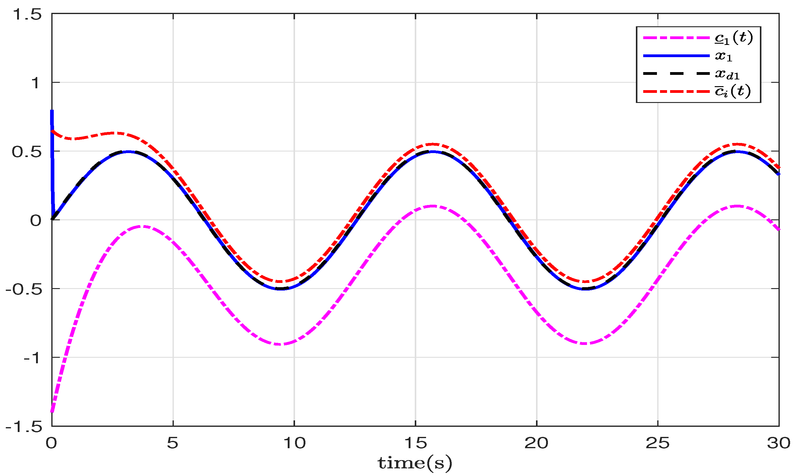
We consider the following MIMO continuous-time completely unknown SPSs:

$$\begin{array}{c}\hfill \left\{\begin{array}{cc}\hfill E\left(\epsilon \right)\dot{x}& =F\left(x\right)+G\left(x\right)u\hfill \\ \hfill y& =x\hfill \end{array}\right.\end{array}$$

(1)

where $E\left(\epsilon \right)=[I_{n_1\times n_1}0;0\epsilon I_{n_2\times n_2}]\in R^{n\times n}(n_1+n_2=n)$, $0<\epsilon <1$ represents the SPP, $x=[x_s^T,x_f^T]\in R^n$ is the states of the SPS nonlinear, where $x_s$ and $x_f$ denotes “slow” and “fast” system state, respectively, $F\left(x\right)=[F_s\left(x\right);F_f\left(x\right)]\in R^n$ and $G\left(x\right)=[G_s\left(x\right);G_f\left(x\right)]\in R^{n\times n}$ are smooth but completely unknown nonlinear functions with $F\left(x\right)$ containing all the modeling uncertainties and external disturbances, $u={[u_1,u_2,\cdots ,u_n]}^T\in R^n$ denotes the control input vector, and y is output vector.

The goal of the partial states tracking problem is to design an adaptive NN control policy u for the SPSs to meet the goals below in the presence of ill-conditioned numerical, completely unknown nonlinear functions, and full-state constraints.

• The slow states $x_s$ track a reference trajectory $x_d\left(t\right)\in R^{n_1}$;
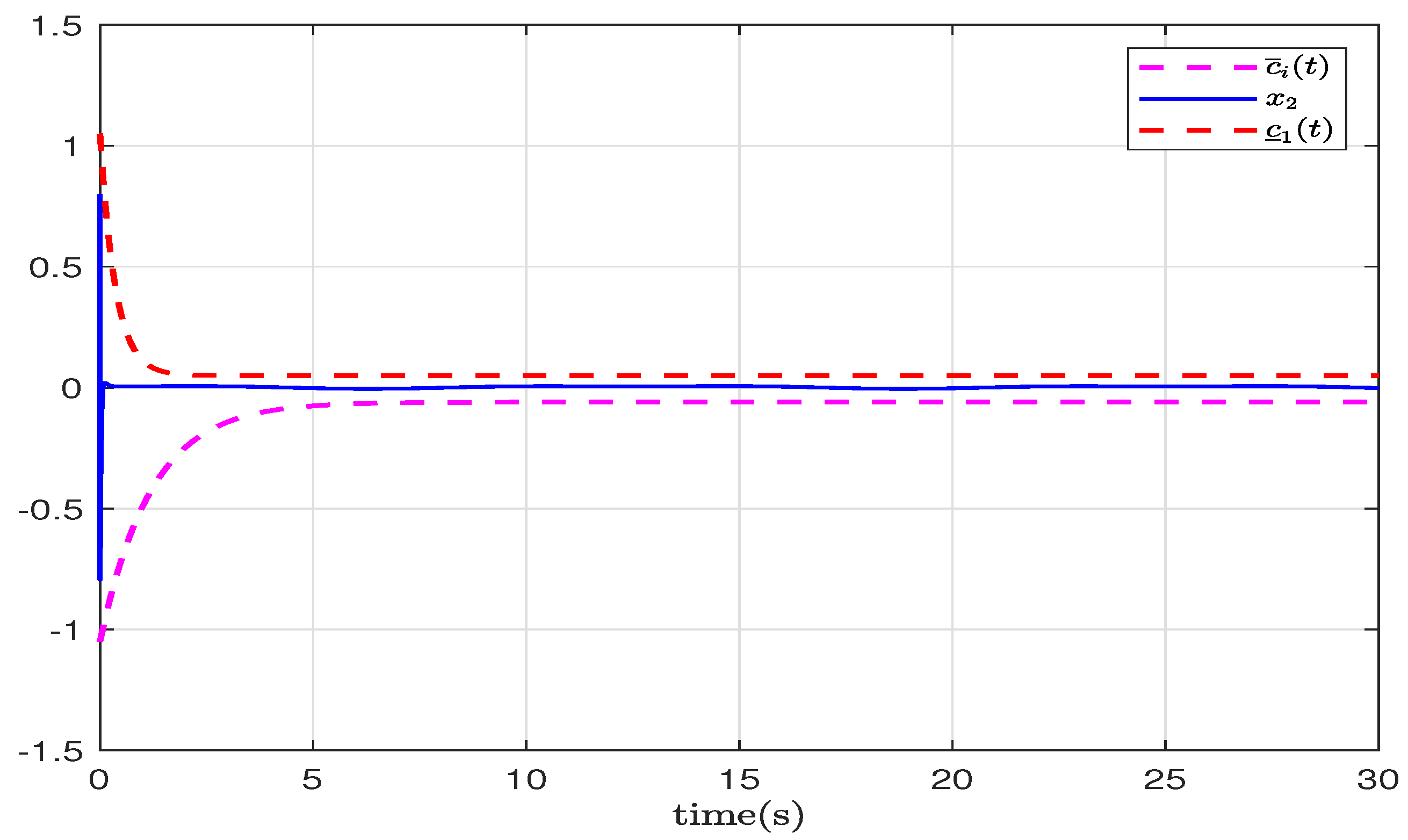
• The full system states are forced to be within the asymmetric and time-varying constraints for all times, e.g.,

  $${\underline{c}}_i\left(t\right)<x_i\left(t\right)<{\overline{c}}_i\left(t\right),i=1,2,\cdots ,n$$

  (2)

  where ${\underline{c}}_i\left(t\right)$ and ${\overline{c}}_i\left(t\right)$ are the lower and upper bounds for the state $x_i\left(t\right)$;
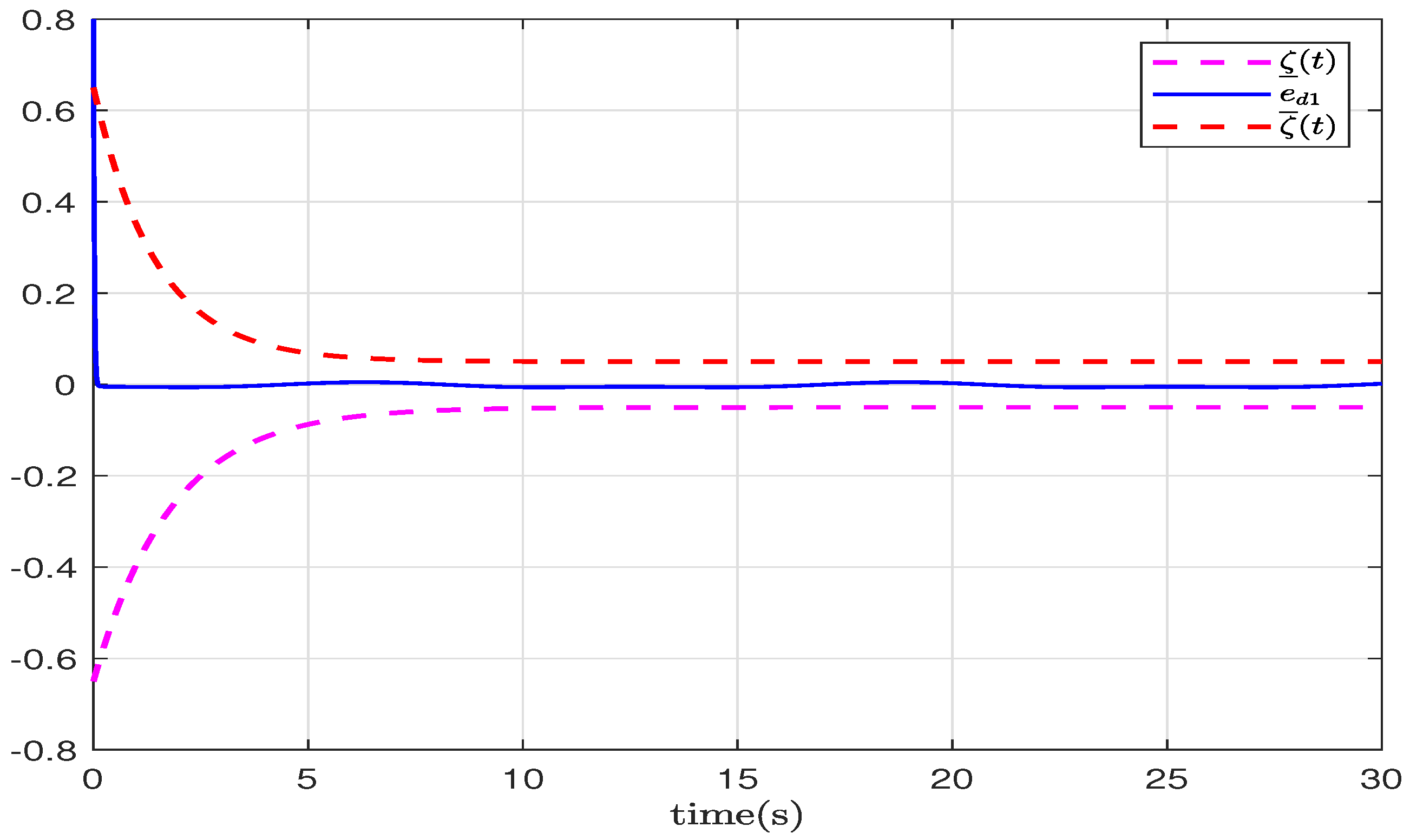
• All the signals in the closed-loop system are semi-globally uniformly ultimately bounded (SGUUB).

Remark 1.

Practically, since the controller matrices involve small SPP, the SPSs (1) may experience abrupt changes in their structures and parameters, which usually leads to low control performance and even instability of the system.

Remark 2.

For actual systems, many states cannot be tracked in advance since they have no actual physical significance. Therefore, this paper studies the tracking problem of a partial system state, that is, the slow state tracks the ideal signal.

Assumption 1.

The matrices $G\left(x\right)$ are definite, and there exist unknown positive constants ${\underline{g}}_0$ and ${\overline{g}}_0$ such that ${\underline{g}}_0<\left|\lambda \left(G\left(x\right)\right)\right|<{\overline{g}}_0,x\in {\Omega }_x$ with ${\Omega }_x$ being a compact set and λ being the eigenvalue operator.

Assumption 2.

The desired trajectory $x_d=[x_{d1},x_{d2},\cdots ,x_{d{n}_1}]$ is continuously differentiable and available for controller design.

Assumption 3.

The bounds ${\underline{c}}_i\left(t\right)$ and ${\overline{c}}_i\left(t\right)$ are smooth functions with their n-th derivatives available for controller design.

2.2. Neural Network Online Approximation

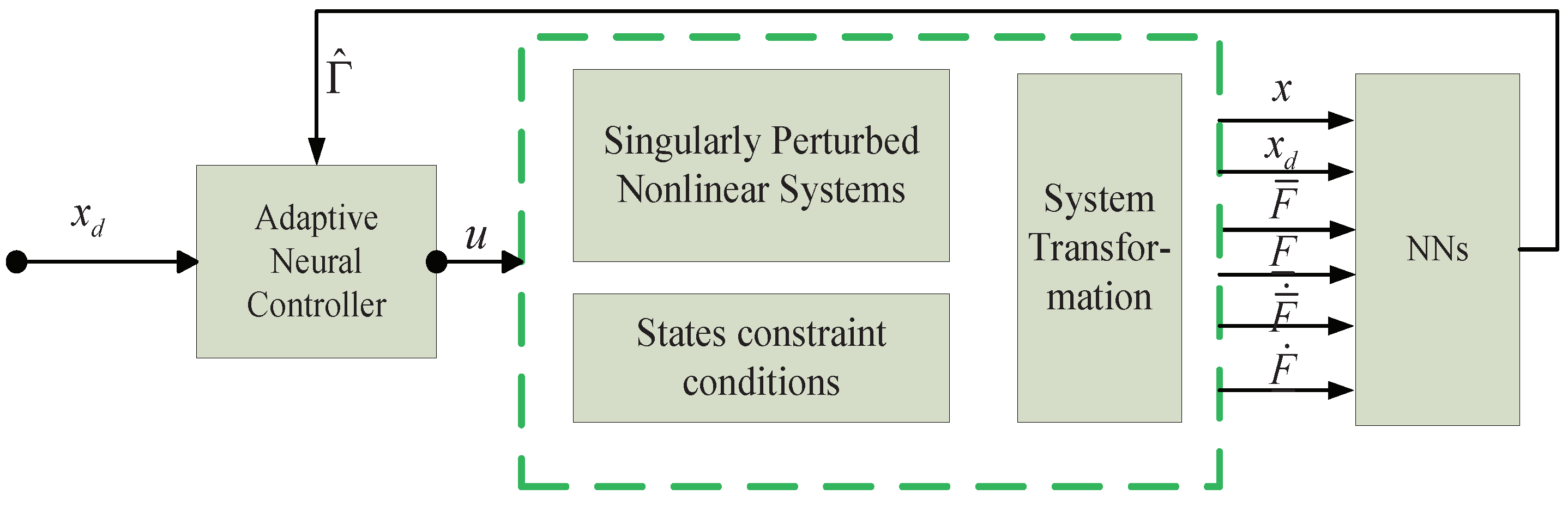
Due to the advantages of NNs in function approximation [48,49,50], we can use them to estimate unknown nonlinear functions in uncertain MIMO nonlinear SPSs [23,24]. Consider continuous function $h\left(X\right):R^n\to R$, approximated by NN

$$\begin{array}{c}\hfill h_{nn}\left(X\right)={\widehat{W}}^{T}S\left(X\right)\end{array}$$

(3)

where $X\in {\mathbb{R}}^n$ is the NN input variable, $\widehat{W}={[{\widehat{w}}_1,{\widehat{w}}_2,\cdots ,{\widehat{w}}_p]}^T\in R^p$ is the NN weight vector with $p>1$ being the number of hidden layer nodes. $S\left(X\right)={[S_1\left(X\right),S_2\left(X\right),\cdots ,S_p\left(X\right)]}^T\in R^p$, $S_i(·)$ is the commonly named activation function, which is selected by the Gaussian function in our article, i.e., $S_i\left(X\right)=\exp (-{(X-{\mu }_i)}^T(X-{\mu }_i)/{\sigma }_i^2)$, where ${\mu }_i={[{\mu }_{i1},{\mu }_{i2},\cdots ,{\mu }_{il}]}^T$$\in R^l$ and ${\sigma }_i$ denotes adjustable parameters of the Gaussian function $S_i\left(X\right)$. According to the definition of activation function $S\left(X\right)$, there exists a constant $\zeta$ such that

$$\begin{array}{c}\hfill S{\left(X\right)}^{T}S\left(X\right)\le \zeta \end{array}$$

(4)

As a general rule, if l is large enough, and ${\mu }_i$ and ${\sigma }_i$ are appropriately chosen, NN (3) is capable of approximating any continuous function $h\left(X\right):R^n\to R$ with any arbitrary accuracy

$$\begin{array}{c}\hfill h\left(X\right)=W^{\ast T}S\left(X\right)+{\epsilon }_X\end{array}$$

(5)

over a compact set ${\Omega }_X\subset R^n$, where $W^{\ast }$ denotes the optimal constant weight vector of the output layer, and ${\epsilon }_X$ is the approximation error such that $|{\epsilon }_X|\le \overline{\epsilon }$, where ${\epsilon }_X>0$ is unknown and only used for analytical purpose. For all $X\in {\Omega }_X\subset {\mathbb{R}}^n$, the ideal weight $W^{\ast }$ can be defined as:

$$\begin{array}{c}\hfill W^{\ast }:=arg\underset{\widehat{W}\in R^l}{min}\left\{\underset{X\in R^n}{sup}|h\left(X\right)-h_{nn}(\widehat{W},X)|\right\}\end{array}$$

(6)

Remark 3.

To overcome the nonlinear, complex, multi-variable, uncertain dynamics systems, refs. [51,52] have studied the design of fractional-order control for photovoltaic (PV)/battery systems with the help of type-3 fuzzy logic systems. Type-3 fuzzy logic system has one more degree of freedom and can deal with higher-order and complex uncertainty, so the type-3 fuzzy logic controller can obtain better control performance and have higher robustness. Inspired by this, we will use the type-3 fuzzy logic systems to deal with the higher-order uncertainty in future research to improve the control performance.

3. Main Results

To ensure that the pre-defined range (2) is satisfied, a new system transformation method is proposed, which converts the original SPSs (1) with state constraints into a new SPSs with no constraints. Thus, if we guarantee the stability of the new system, we can achieve the asymmetrical yet time-varying state constraints.

3.1. System Transformation

The tracking error between the actual and the desired outputs is defined as

$$e_d\left(t\right)=x_s\left(t\right)-x_d\left(t\right)$$

(7)

where $e_d\left(t\right)={[e_{d1},\cdots ,e_{d{n}_1}]}^T\in R^{n_1}$ and $x_{dj}$ satisfies

$${\underline{c}}_j\left(t\right)<x_{dj}<{\overline{c}}_j\left(t\right)$$

(8)

Subtract $x_{dj}$ from both sides of (2) and yield

$${\underline{c}}_j\left(t\right)-x_{dj}<e_{dj}\left(t\right)<{\overline{c}}_j\left(t\right)-x_{dj}$$

(9)

where $j=1,2,\cdots ,n_1$. Define ${\underline{\zeta }}_j\left(t\right)={\underline{c}}_j\left(t\right)-x_{dj}$, ${\overline{\zeta }}_j\left(t\right)={\overline{c}}_j\left(t\right)-x_{dj}$, where ${\underline{\zeta }}_j\left(t\right)<0$ and ${\overline{\zeta }}_j\left(t\right)>0$. Equation (9) turns into

$${\underline{\zeta }}_j\left(t\right)<e_{dj}\left(t\right)<{\overline{\zeta }}_j\left(t\right)$$

(10)

In this way, the state constraints (2) of the original systems are converted to the tracking error constraints described by (10). Considering Equation (7) and system (1), we have

$$\begin{array}{cc}\hfill E\left(\epsilon \right)\dot{\chi }& =\mathcal{F}\left(x\right)+G\left(x\right)u\hfill \end{array}$$

(11)

where $\chi =[(e_d{\left(t\right)}^T,x_f^T]\in R^n$, $\mathcal{F}\left(x\right)=[F_s\left(x\right)-x_d\left(t\right);F_f\left(x\right)]$.

To eliminate the feasibility conditions on the virtual control based on the error transformation technique, we investigate the state constraints design control for tracking error $e_{dj}$ subject to (10) and $x_f$ subject to (2). Assume that ${\mathbb{C}}_{1j},j=1,\cdots ,n$ is the initial conditions of the nonlinear SPSs (1). By introducing time-varying asymmetric constraints functions ${\xi }_i$ that only depend on $\chi$, we directly implement the time-varying asymmetric state constraints for system (11)

$$\begin{array}{c}\hfill {\xi }_i\left(t\right)=\frac{{\chi }_{1i}+{\underline{k}}_i}{{\chi }_{1i}+{\underline{F}}_i\left(t\right)}+\frac{{\chi }_{1i}-{\overline{k}}_i}{{\overline{F}}_i\left(t\right)-{\chi }_{1i}},i=1,2,\cdots ,n\end{array}$$

(12)

where ${\underline{F}}_j\left(t\right)={\underline{\zeta }}_j\left(t\right)$, ${\overline{F}}_j\left(t\right)={\overline{\zeta }}_j\left(t\right),j=1,2,\cdots ,n_1$, ${\underline{F}}_v\left(t\right)={\underline{c}}_v\left(t\right)$, ${\overline{F}}_v\left(t\right)={\overline{c}}_v\left(t\right)$, $v=n_1+1,n_2+2,\cdots ,n_2$, ${\underline{k}}_i$ and ${\overline{k}}_i$ are constants and satisfy ${\underline{k}}_i<{\underline{F}}_i\left(t\right)$ and ${\overline{k}}_i<{\overline{F}}_i\left(t\right)$. From (12), it is seen that ${\beta }_i\left(t\right)$ tend to infinity when $x_{1i}\to {\underline{F}}_i\left(t\right)$ or ${\chi }_{1i}\to {\overline{F}}_i\left(t\right)$, and ${\beta }_i\left(t\right)$ are bounded if ${\chi }_{1i}\left(t\right)\in {\mathbb{C}}_{1i}^{{}^{\prime }}⫋{\mathbb{C}}_{1i}$. Under the initial condition ${\chi }_{1i}\left(0\right)\in {\mathbb{C}}_{1i}^{{}^{\prime }}⫋{\mathbb{C}}_{1i}$, it can be seen that ${\chi }_{1i}\left(t\right)\in {\mathbb{C}}_{1i}$ if ${\xi }_i\left(t\right)\in L_{\infty }$ for $\forall t\ge 0$, which implies that asymmetric yet time-varying output constraints are achieved. Now, the problem turns to how to guarantee ${\xi }_i\left(t\right)$ to be bounded.

Differentiating ${\xi }_i\left(t\right)$ with respect to t yields

$$\begin{array}{cc}\hfill {\xi }_i\left(t\right)& ={\psi }_{1i}\left(t\right){\dot{\chi }}_{1i}\left(t\right)+{\psi }_{2i},i=1,2,\cdots ,n\hfill \end{array}$$

(13)

with

$${\psi }_{1i}\left(t\right)=\frac{{\underline{F}}_i\left(t\right)-{\underline{k}}_i}{{({\chi }_{1i}\left(t\right)+{\underline{F}}_i\left(t\right))}^2}+\frac{{\overline{F}}_i\left(t\right)-{\overline{k}}_i}{{({\overline{F}}_i\left(t\right)-{\chi }_{1i}\left(t\right))}^2}$$

(14)

$${\psi }_{2i}\left(t\right)=-\frac{({\chi }_{1i}\left(t\right)+{\underline{k}}_i){\dot{\underline{F}}}_i\left(t\right)}{{({\chi }_{1i}\left(t\right)+{\underline{F}}_i\left(t\right))}^2}-\frac{({\chi }_{1i}\left(t\right)-{\overline{k}}_i){\dot{\overline{F}}}_i\left(t\right)}{{({\overline{F}}_i\left(t\right)-{\chi }_{1i}\left(t\right))}^2}$$

(15)

It can be used for control design in the set ${\chi }_{1i}\in {\mathbb{C}}_{1i}$. Equivalently, Equation (13) is also written as a vector as follows

$$\begin{array}{c}\hfill \xi ={\psi }_1{\dot{\chi }}_1+{\psi }_2\end{array}$$

(16)

where ${\psi }_1=diag\left\{[{\psi }_{11},{\psi }_{12},\cdots ,{\psi }_{1n}]\right\}\in {\mathbb{R}}^{n\times n}$, ${\psi }_2=[{\psi }_{21},{\psi }_{22},\cdots ,{\psi }_{2n}]\in {\mathbb{R}}^n$, and $\xi ={[{\xi }_1,{\xi }_2,\cdots ,{\xi }_n]}^T\in {\mathbb{R}}^n$.

Then, the system (1) under partial state tracking can be expressed as the following dynamic systems:

$$\begin{array}{cc}\hfill & \left\{\begin{array}{cc}\hfill E\left(\epsilon \right)\dot{\xi }& ={\psi }_1[\mathcal{F}\left(x\right)+G\left(x\right)u]+{\psi }_2\hfill \\ \hfill y& =x\hfill \end{array}\right.\hfill \end{array}$$

(17)

3.2. Adaptive Controller Design and Stability Analysis

In the subsection, a novel NNs-based adaptive partial states tracking control approach of uncertain MIMO nonlinear SPSs (1) possessing constraint condition (2) is proposed. For that purpose, coordinate transformation is defined as follows

$$V_1=\frac{1}{2}{\xi }^{T}E{\left(\epsilon \right)}^{T}P\xi$$

(18)

where $P=[P_{11},\epsilon P_{12};P_{12}^T,P_{22}]$ such that

$$E{\left(\epsilon \right)}^{T}P=P^{T}E\left(\epsilon \right)$$

(19)

The derivative of $V_1$ along (17) and (19) is

$$\begin{array}{cc}\hfill {\dot{V}}_1& ={\xi }^{T}E{\left(\epsilon \right)}^{T}P\dot{\xi }\hfill \\ \hfill & ={\xi }^T{P}^T\{{\psi }_1[\mathcal{F}\left(x\right)+G\left(x\right)u]+{\psi }_2\}\hfill \\ \hfill & ={\xi }^T{P}^T{\psi }_1\{[\mathcal{F}\left(x\right)+G\left(x\right)u]+{\psi }_1^{-1}{\psi }_2\}\hfill \\ \hfill & ={\xi }^T{P}^T{\psi }_{1}G\left(x\right)\{G{\left(x\right)}^{-1}[\mathcal{F}\left(x\right)+{\psi }_1^{-1}{\psi }_2]+u\}\hfill \end{array}$$

(20)

where $\mathcal{F}\left(x\right)$, $G\left(x\right)$ are unknown and how to eliminate the uncertainty is a significant challenge. We approximate $\mathcal{F}\left(x\right)$ and $G\left(x\right)$ by the aforementioned NNs by using the information of available state $x_1$. For clarity, (20) can be rewrite as

$$\begin{array}{cc}\hfill {\dot{V}}_1& ={\xi }^T{P}^T{\psi }_{1}G\left(x\right)(\Gamma +u)\hfill \end{array}$$

(21)

where $\Gamma \left({\rm Y}\right)=G{\left(x\right)}^{-1}[\mathcal{F}\left(x\right)+{\psi }_1^{-1}{\psi }_2]$ with ${\rm Y}=[x^T,x_d^T,\underline{F}{\left(t\right)}^T,\overline{F}\left(t\right),\dot{\underline{F}}{\left(t\right)}^T,\dot{\overline{F}}\left(t\right)]\in R^{6n}$. It goes without saying that function $\Gamma \left({\rm Y}\right)$ is unknown. Therefore, to eliminate the high degree of uncertainty in the system and provide an executable controller for the system, NNs are utilized to approximate $\Gamma \left({\rm Y}\right)$, that is

$$\begin{array}{c}\hfill \Gamma \left({\rm Y}\right)=W^{\ast T}S\left({\rm Y}\right)+{\epsilon }_{\chi }\end{array}$$

(22)

according to (5), we have that $\parallel W\parallel \le \overline{\omega }$, $\parallel {\epsilon }_{\chi }\parallel \le {\overline{\epsilon }}_{\chi }$ in which $\overline{\omega }$ and ${\overline{\epsilon }}_{\chi }$ are unknown positive constants and are only used for stability analysis. Then, (21) becomes

$$\begin{array}{cc}\hfill {\dot{V}}_1& ={\xi }^T{P}^T{\psi }_{1}G\left(x\right)(W^{\ast T}S\left({\rm Y}\right)+{\epsilon }_{\chi }+u)\hfill \end{array}$$

(23)

Let $\widehat{W}$ be the estimate of $W^{\ast }$, and an implementable controller is presented as:

$$\begin{array}{cc}\hfill u& =-k_1\xi -\widehat{W}S\left({\rm Y}\right)\hfill \end{array}$$

(24)

where $k_1=k_{10}+k_{11}\parallel {\psi }_1\parallel$, the constants $k_{10}>0$, $k_{11}>0$. The adaptive law for $\widehat{W}$ is selected

$$\dot{\widehat{W}}=P\Phi (S\left({\rm Y}\right){\xi }^T-\varrho \parallel \xi \parallel \widehat{W})$$

(25)

where ${\Phi }^T=\Phi >0$ represents the adaptation gain matrix, and $\varrho$ is a small design parameter.

Lemma 1.

For adaptive NNs law (25), there is a compact set such as

$$\begin{array}{c}\hfill \mathcal{C}=\{\widehat{W}|||\widehat{W}||\le \frac{\varpi }{\varrho }\}\end{array}$$

(26)

where $\parallel S\left(\chi \right)\parallel \le \varpi$ with $\varpi >0$, $\widehat{W}\left(t\right)\in \mathcal{C},\forall t\ge 0$ and $\widehat{W}\left(0\right)\in \mathcal{C}$.

Proof. 

Design the positive Lyapuonv function below.

$$\begin{array}{c}\hfill V_{w1}=\frac{1}{2}tr\left({\widehat{W}}^T{(P\Phi )}^{-1}\widehat{W}\right)\end{array}$$

(27)

where $tr(·)$ denotes the matrix trace. The time derivative of $V_{w1}$ is obtained as

$$\begin{array}{cc}\hfill {\dot{V}}_{w1}& =tr\left\{{\widehat{W}}^T\left(S\left({\rm Y}\right){\xi }^T-\varrho \parallel \xi \parallel \widehat{W}\right)\right\}\hfill \\ \hfill & =tr\left({\widehat{W}}^{T}S\left({\rm Y}\right){\xi }^T\right)-\varrho \parallel \xi \parallel tr\left({\widehat{W}}^T\widehat{W}\right)\hfill \\ \hfill & =S{\left({\rm Y}\right)}^T\widehat{W}\xi -\varrho \parallel \xi \parallel {∥\widehat{W}∥}^2\hfill \\ \hfill & \le \parallel \xi \parallel ∥\widehat{W}∥\varpi -\varrho \parallel \xi \parallel {∥\widehat{W}∥}^2\hfill \\ \hfill & =-\parallel \xi \parallel ∥\widehat{W}∥\left(\varrho ∥\widehat{W}∥-\varpi \right)\hfill \end{array}$$

(28)

${\dot{V}}_w$ will be negative as long as $\widehat{W}\parallel <\frac{\varpi }{\varrho }$. Hence, $\widehat{W}\in \mathcal{C}$ if $\widehat{W}\left(0\right)\in C$ for $t>0$. □

Thereafter, substituting the control input (24) into (23) generates

$$\begin{array}{cc}\hfill {\dot{V}}_1& ={\xi }^T{P}^T{\psi }_{1}G\left(x\right)(W^{\ast T}S\left({\rm Y}\right)+{\epsilon }_{\chi }-k_1\xi -\widehat{W}S\left({\rm Y}\right))\hfill \\ \hfill & =-k_1{\xi }^T{P}^T{\psi }_{1}G\left(x\right)\xi -{\xi }^T{P}^T{\psi }_{1}G\left(x\right){\tilde{W}}^{T}S\left({\rm Y}\right)\hfill \\ \hfill & +{\xi }^T{P}^T{\psi }_{1}G\left(x\right){\epsilon }_{\chi }\hfill \end{array}$$

(29)

where $\tilde{W}=\widehat{W}-W^{\ast }$.

As implied in Lemma 1, ${\widehat{W}}_1$ is bounded. Then, following Assumption 1, it holds that $∥{\tilde{W}}_1∥\le {ϵ}_{w1}$ with the constant ${ϵ}_{w1}>0$ is unknown. In addition, $∥S\left({\rm Y}\right)∥\le {\varphi }_{m1}$ and $∥{ϵ}_1∥<{ϵ}_{m1}$. Due to the fact that the diagonal matrix $R>0$ and $G_1\left(x_1\right)>0$, it comes that $R{G}_1\left(x_1\right)>0$. Thus, ${\dot{V}}_1$ can be further rewritten as

$$\begin{array}{cc}\hfill {\dot{V}}_1& \le -k_1{\parallel \xi \parallel }^2{\lambda }_{min}\left(P^T{\psi }_1{G}_1\left(x_1\right)\right)+\parallel \xi \parallel \parallel {\psi }_1\parallel {\lambda }_{max}\left(G_1\left(x_1\right)\right)m_1\hfill \end{array}$$

(30)

with $m_1=\varpi {ϵ}_{w1}+{ϵ}_{w1}$. Using $k_1$, Equation (30) is derived as

$$\begin{array}{cc}\hfill {\dot{V}}_1\le & -\left(k_{10}+k_{11}{\parallel {\psi }_1\parallel }^2\right){\parallel \xi \parallel }^2{\lambda }_{min}\left({\psi }_1{G}_1\left(x_1\right)\right)\hfill \\ \hfill & +\parallel \xi \parallel \parallel {\psi }_1\parallel {\lambda }_{max}\left(G_1\left(x_1\right)\right)m_1\hfill \\ \hfill =& -k_{10}{\parallel \xi \parallel }^2{\lambda }_{min}\left({\psi }_1{G}_1\left(x_1\right)\right)-k_{11}^{\ast }\parallel {\psi }_1{\parallel }^2{\parallel \xi \parallel }^2\hfill \\ \hfill & +\parallel {\psi }_1\parallel \parallel s\parallel m_1^{\ast }\hfill \end{array}$$

(31)

where $k_{11}^{\ast }=k_{11}{\lambda }_{min}\left({\psi }_1{G}_1\left(x_1\right)\right)$, and $m_1^{\ast }={\lambda }_{max}\left(G_1\left(x_1\right)\right)m_1$. Utilizing the completion of squares, it becomes

$$-k_{11}^{\ast }{\parallel R\parallel }^2{\parallel s\parallel }^2+\parallel R\parallel \parallel s\parallel m_1^{\ast }\le \frac{m_1^{\ast 2}}{4k_{11}^{\ast }}$$

Thus, it follows that

$$\begin{array}{cc}\hfill {\dot{V}}_1\le & -k_{10}{\lambda }_{min}\left({\psi }_1{G}_1\left(x_1\right)\right)+\frac{m_1^{\ast 2}}{4k_{11}^{\ast }}\hfill \end{array}$$

(32)

Theorem 1.

Consider the system (1) satisfying Assumptions 1–3. Using the controller (24) and adaptive NNs law (25), we have

• The full state constraints of the system are maintained in (2);
• The boundedness of all signals in the closed-loop system are guaranteed.

Proof. 

Choose a Lyapunov function.

$$\begin{array}{cc}\hfill V& =V_1=\frac{1}{2}{\xi }^{T}E{\left(\epsilon \right)}^{T}P\xi \hfill \end{array}$$

(33)

Following (32), we have

$$\begin{array}{cc}\hfill \dot{V}& \le -k_{10}{\lambda }_{min}\left({\psi }_1{G}_1\left(x_1\right)\right){\parallel \xi \parallel }^2+\frac{m_1^{\ast 2}}{4k_{11}^{\ast }}\hfill \\ \hfill & =-CV+\zeta \hfill \end{array}$$

(34)

where $C=k_{10}{\lambda }_{min}\left({\psi }_1{G}_1\left(x_1\right)\right)$ and $\zeta =\frac{m_1^{\ast 2}}{4k_{11}^{\ast }}$. It can be seen from (34) that the signals $e_d$ and $\dot{\widehat{W}}$ are bounded. Notice that $u\in L_{\infty }$ in a compact set ${\mathcal{C}}_{di}:=\{(t,y_{dj})\in {\mathbb{R}}_{+}\times \mathbb{R}|-{\underline{c}}_j\left(t\right)\le x_{dj}\left(t\right)\le {\overline{c}}_j\left(t\right),j=1,2,\cdots ,n_1\}\}$ and $e_d=x_s-x_d$. Then it is guaranteed that $\beta \in L_{\infty }$. Hence, under the initial conditions $x_{1i}\left(0\right)\in {\mathbb{C}}_{1i},i=1,2,\cdots ,n$, the state x does not violate state constraints (2), i.e., it remains in the pre-given constrained space ${\mathbb{C}}_{1j}$.

Furthermore, according to $e_1=[e_{11},e_{12},\cdots ,e_{1n}]\in R^n$, we get

$$\begin{array}{cc}\hfill e_{1i}& =\left(\frac{{\underline{F}}_i-{\underline{k}}_i}{(x_{1i}+{\underline{F}}_i)(x_{di}+{\underline{F}}_i)}+\frac{{\overline{F}}_i-{\overline{k}}_i}{({\overline{F}}_i-x_{1i})({\overline{F}}_i-x_{di})}\right){\zeta }_{1i}\hfill \end{array}$$

which can be expressed as

$$\begin{array}{c}\hfill e_{1i}={\varpi }_i{\zeta }_{1i}\end{array}$$

(35)

where ${\varpi }_i=({\underline{F}}_i-{\underline{k}}_i)/\left((x_{1i}+{\underline{F}}_i)(x_{di}+{\underline{F}}_i)\right)+({\overline{F}}_i-{\overline{k}}_i)/\left(({\overline{F}}_i-x_{1i})({\overline{F}}_i-x_{di})\right)$. According to Assumption 2, the positive constants ${\overline{\vartheta }}_{1i}$, ${\underline{\vartheta }}_{1i}$, ${\overline{\vartheta }}_{2i}$ and ${\underline{\vartheta }}_{2i}$ satisfy ${\overline{\vartheta }}_{1i}\ge {\underline{F}}_i\left(t\right)-{\underline{k}}_i\ge {\underline{\vartheta }}_{1i}>0$ and ${\overline{\vartheta }}_{2i}\ge {\overline{F}}_i\left(t\right)-{\overline{k}}_i\ge {\overline{\vartheta }}_{2i}>0$. Additionally, based on the above analysis, it is easy to see that $x_{1i}$ is in the subset of ${\mathbb{C}}_{1i},i=1,2,\cdots ,n$, which shows that the positive constants ${\underline{\vartheta }}_{3i}$, ${\overline{\vartheta }}_{3i}$, ${\underline{\vartheta }}_{4i}$ and ${\overline{\vartheta }}_{4i}$ such that $0<{\underline{\vartheta }}_{3i}\le (x_{1i}+{\underline{F}}_i)(x_{di}+{\underline{F}}_i)\le {\overline{\vartheta }}_{3i}$ and $0<{\underline{\vartheta }}_{4i}\le ({\overline{F}}_i-x_{1i})({\overline{F}}_i-x_{di})\le {\overline{\vartheta }}_{4i}$, this further shows that the positive constants ${\overline{\varrho }}_i$ and ${\underline{\varrho }}_i$ satisfy $0<{\underline{\varrho }}_i<{\varpi }_i<{\overline{\varrho }}_i$. Then, it shows from (35) that ${\zeta }_{1i}$ is bounded as $e_{1i}\in L_{\infty }$. □

4. Simulation

A nonlinear circuit is used to validate the effectiveness of the adaptive controller for MIMO uncertain SPSs possessing state constraints, whose state equations are as follows

$$\begin{array}{cc}\hfill \mathcal{L}{\dot{I}}_{\mathcal{L}}& =-I_{\mathcal{L}}\mathcal{R}-{\upsilon }_c+u\left(t\right)\hfill \\ \hfill \mathcal{C}{\dot{\upsilon }}_c\left(t\right)& =I_{\mathcal{L}}-\frac{1}{5}({\upsilon }_c^3-{\upsilon }_c)+\gamma u\left(t\right)\hfill \end{array}$$

(36)

where $\gamma =0.5,\mathcal{R}=2\Omega$ and $\mathcal{L}=0.1H$. Let $\mathcal{C}=\epsilon$, ${\zeta }_1\left(t\right)=\mathcal{L}·I_{\mathcal{L}}$ and ${\zeta }_2\left(t\right)={\nu }_c$. Equation (36) comes to the following nonlinear SPSs

$$\begin{array}{cc}\hfill \dot{{\zeta }_1}\left(t\right)& =-20{\zeta }_1\left(t\right)-z\left(t\right)+u\left(t\right)\hfill \\ \hfill \epsilon \dot{{\zeta }_2}\left(t\right)& =10{\zeta }_1\left(t\right)-0.2({\zeta }_2^2\left(t\right)-1){\zeta }_2\left(t\right)+0.5u\left(t\right)\hfill \end{array}$$

which can be rewritten as

$$E\left(ϵ\right)\left[\begin{array}{c}{\dot{\zeta }}_1\\ {\dot{\zeta }}_2\end{array}\right]=\left[\begin{array}{c}-20{\zeta }_1^2-{\zeta }_2\\ 10{\zeta }_1-0.2({\zeta }_2^2-1){\zeta }_2\end{array}\right]+\left[\begin{array}{c}10\\ 00.5\end{array}\right]u$$

(37)

where $E\left(ϵ\right)=\left[\begin{array}{c}10\\ 0\epsilon \end{array}\right]$, $\zeta ={[{\zeta }_1,{\zeta }_2]}^T\in R^2$, initial state condition $\zeta \left(0\right)={[0,0]}^T$, $\epsilon =0.001$, $u\in R^2$. Our purpose is to design an adaptive full state constraints tracking controller for (37) to achieve: (1) the state $x_s$ possessing state constraints follows the desired signal $x_d=0.5sin\left(0.5t\right)$; (2) the boundedness of all signals of the closed-loop system are not violated.

In order to guarantee the reliability of the nonlinear circuit system, its system states must satisfy the following constraints

$$\begin{array}{c}\hfill x_1\in {\mathcal{D}}_{11}:=\{{\zeta }_1\in R:-{\underline{F}}_{c1}<{\zeta }_1<{\overline{F}}_{c1}\}\end{array}$$

(38)

$$\begin{array}{c}\hfill x_2\in {\mathcal{D}}_{12}:=\{{\zeta }_2\in R:-{\underline{F}}_{c2}<{\zeta }_2<{\overline{F}}_{c2}\}\end{array}$$

(39)

where ${\underline{F}}_{c1}=-2^{-0.8t}-0.05+x_d\left(t\right)$, ${\overline{F}}_{c1}=-0.99\times 2^{-t}+0.04+x_d\left(t\right)$, ${\underline{F}}_{c2}=-0.99\times 2^{-1.2t}-0.06$, and ${\overline{F}}_{c2}=2^{-4t}+0.05$. Set the initial condition $\zeta \left(0\right)={[{\zeta }_s\left(0\right),{\zeta }_f\left(0\right)]}^T={[0.8,0.8]}^T$. $\widehat{W}\left(0\right)$ is selected as $11.5$. Choose the design parameters: $E\left(\epsilon \right)=[10;00.1],$ $P_{11}=6$, $P_{12}=10,P_{22}=7$, ${\rho }_1=9$, ${\rho }_2=10$, ${\gamma }_1=0.1$, ${\gamma }_2=0.2$.

The general block diagram is shown in Figure 1. We display the simulation results for the nonlinear circuit (36) with the parasitic capacitor and nonlinear resistor. Figure 2 and Figure 3 express the curves of state $\zeta ={[{\zeta }_s^T,{\zeta }_f^T]}^T$ satisfying the constraint regions (38) and (39), which shows with the updating law (25) that the system states do not violate the predefined time-varying yet asymmetric region. The tracking error $e_d={\zeta }_s-{\zeta }_d$ is plotted in Figure 4. The response curves of the designed control inputs are shown in Figure 5. We select the activation function $S(·)$ as the Gaussian function. The $L_2$ norm of the updated parameters $\widehat{W}$ is plotted in Figure 6. Furthermore, the systems state ${\zeta }_2$ (fast dynamic states ) are shown in Figure 3. It shows that satisfactory tracking performance is ensured while possessing time-varying state constraints.

5. Conclusions

For nonlinear SPSs with unknown functions, we thoroughly solve the full-state constrained partial tracking control issue without introducing the feasibility conditions. The key feature of the designed algorithm lies in that the original state constrained control with respect to the partial state tracking error system is converted into a stabilization one. We have proved that slow state tracking is met with its state evolved in a pre-given time-varying constraint boundaries. In addition, the closed-loop system signals are SGUUB along with the ill-conditioned numerical, which was prevented via specially designing an $\epsilon$-dependent Lyapunov function. Finally, a practical system example indicates the satisfactory control performance.

References

1. Ren, W.; Jiang, B.; Yang, H. Singular perturbation-based fault-tolerant control of the air-breathing hypersonic vehicle. IEEE/ASME Trans. Mechatronics 2019, 24, 2562–2571. [Google Scholar] [CrossRef]
2. Van Henten, E.J.; Bontsema, J. Time-scale decomposition of an optimal control problem in greenhouse climate management. Control Eng. Pract. 2009, 17, 88–96. [Google Scholar] [CrossRef]
3. Ren, W.; Jiang, B.; Yang, H. Fault-tolerant control of singularly perturbed systems with applications to hypersonic vehicles. IEEE Trans. Aerosp. Electron. Syst. 2019, 55, 3003–3015. [Google Scholar] [CrossRef]
4. Xu, J.; Lim, C.C.; Shi, P. Sliding mode control of singularly perturbed systems and its application in quad-rotors. Int. J. Control 2019, 92, 1325–1334. [Google Scholar] [CrossRef]
5. Ma, L.; Wang, Z.; Cai, C.; Alsaadi, F.E. Dynamic event-triggered state estimation for discrete-time singularly perturbed systems with distributed time-delays. IEEE Trans. Syst. Man Cybern. Syst. 2018, 50, 3258–3268. [Google Scholar] [CrossRef]
6. Rejeb, J.B.; Morărescu, I.C.; Daafouz, J. Control design with guaranteed cost for synchronization in networks of linear singularly perturbed systems. Automatica 2018, 91, 89–97. [Google Scholar] [CrossRef] [Green Version]
7. Liu, X.; Yang, C.; Zhou, L.; Dai, W. Suboptimal reduced control of unknown nonlinear singularly perturbed systems via reinforcement learning. Int. J. Robust Nonlinear Control 2021, 31, 6626–6645. [Google Scholar] [CrossRef]
8. Yang, C.; Zhong, S.; Liu, X.; Zhou, L. Adaptive composite suboptimal control for linear singularly perturbed systems with unknown slow dynamics. Int. J. Robust Nonlinear Control 2020, 30, 2625–2643. [Google Scholar] [CrossRef]
9. Liu, X.; Yang, C.; Zhu, S. Inverse optimal synchronization control of competitive neural networks with constant time delays. Neural Comput. Appl. 2022, 34, 241–251. [Google Scholar] [CrossRef]
10. Lei, Y.; Wang, Y.W.; Morarescu, I.C.; Postoyan, R. Event-triggered fixed-time stabilization of two-time-scale linear systems. IEEE Trans. Autom. Control 2022. [Google Scholar] [CrossRef]
11. Cheng, J.; Yan, H.; Park, J.H.; Zong, G. Output-feedback control for fuzzy singularly perturbed systems: A nonhomogeneous stochastic communication protocol approach. IEEE Trans. Cybern. 2021. [Google Scholar] [CrossRef]
12. Wang, Y.; Shi, P.; Yan, H. Reliable control of fuzzy singularly perturbed systems and its application to electronic circuits. IEEE Trans. Circuits Syst. I Regul. Pap. 2018, 65, 3519–3528. [Google Scholar] [CrossRef]
13. Shen, H.; Li, F.; Wu, Z.G.; Sreeram, V. Fuzzy-model-based nonfragile control for nonlinear singularly perturbed systems with semi-Markov jump parameters. IEEE Trans. Fuzzy Syst. 2018, 26, 3428–3439. [Google Scholar] [CrossRef]
14. Chen, J.; He, C. Modeling, Fault Detection and Fault-tolerant Control for Nonlinear Singularly Perturbed Systems with Actuator Faults and External Disturbances. IEEE Trans. Fuzzy Syst. 2021. [Google Scholar] [CrossRef]
15. Liu, X.; Yang, C.; Luo, B.; Dai, W. Suboptimal control for nonlinear slow-fast coupled systems using reinforcement learning and Takagi–Sugeno fuzzy methods. Int. J. Adapt. Control Signal Process. 2021, 35, 1017–1038. [Google Scholar] [CrossRef]
16. Wang, J.; Yang, C.; Xia, J.; Shen, H. Observer-based sliding mode control for networked fuzzy singularly perturbed systems under weighted try-once-discard protocol. IEEE Trans. Fuzzy Syst. 2021. [Google Scholar] [CrossRef]
17. Fu, Z.J.; Xie, W.F.; Luo, W.D. Robust on-line nonlinear systems identification using multilayer dynamic neural networks with two-time scales. Neurocomputing 2013, 113, 16–26. [Google Scholar] [CrossRef]
18. Fu, Z.J.; Xie, W.F.; Han, X.; Luo, W.D. Nonlinear systems identification and control via dynamic multitime scales neural networks. IEEE Trans. Neural Netw. Learn. Syst. 2013, 24, 1814–1823. [Google Scholar] [CrossRef]
19. Han, X.; Xie, W.F.; Fu, Z.; Luo, W. Nonlinear systems identification using dynamic multi-time scale neural networks. Neurocomputing 2011, 74, 3428–3439. [Google Scholar] [CrossRef]
20. Song, S.; Zhang, B.; Song, X.; Zhang, Y.; Zhang, Z.; Li, W. Fractional-order adaptive neuro-fuzzy sliding mode H control for fuzzy singularly perturbed systems. J. Frankl. Inst. 2019, 356, 5027–5048. [Google Scholar] [CrossRef]
21. Fu, Z.; Xie, W.; Rakheja, S.; Na, J. Observer-based adaptive optimal control for unknown singularly perturbed nonlinear systems with input constraints. IEEE/CAA J. Autom. Sin. 2017, 4, 48–57. [Google Scholar] [CrossRef]
22. Fu, Z.; Xie, W.; Rakheja, S.; Zheng, D.D. Adaptive optimal control of unknown nonlinear systems with different time scales. Neurocomputing 2017, 238, 179–190. [Google Scholar] [CrossRef]
23. Zheng, D.; Xie, W.; Ren, X.; Na, J. Identification and control for singularly perturbed systems using multitime-scale neural networks. IEEE Trans. Neural Netw. Learn. Syst. 2016, 28, 321–333. [Google Scholar] [CrossRef]
24. Zheng, D.D.; Xie, W.F.; Chai, T.; Fu, Z. Identification and trajectory tracking control of nonlinear singularly perturbed systems. IEEE Trans. Ind. Electron. 2016, 64, 3737–3747. [Google Scholar] [CrossRef]
25. Zheng, D.D.; Fu, Z.J.; Xie, W.F.; Luo, W.D. Indirect adaptive control of nonlinear system via dynamic multilayer neural networks with multi-time scales. Int. J. Adapt. Control Signal Process. 2015, 29, 505–523. [Google Scholar] [CrossRef]
26. Burger, M.; Guay, M. Robust constraint satisfaction for continuous-time nonlinear systems in strict feedback form. IEEE Trans. Autom. Control 2010, 55, 2597–2601. [Google Scholar] [CrossRef]
27. Mayne, D.Q.; Rawlings, J.B.; Rao, C.V.; Scokaert, P.O. Constrained model predictive control: Stability and optimality. Automatica 2000, 36, 789–814. [Google Scholar] [CrossRef]
28. Bemporad, A. Reference governor for constrained nonlinear systems. IEEE Trans. Autom. Control 1998, 43, 415–419. [Google Scholar] [CrossRef] [Green Version]
29. Tee, K.P.; Ge, S.S.; Tay, E.H. Barrier Lyapunov functions for the control of output-constrained nonlinear systems. Automatica 2009, 45, 918–927. [Google Scholar] [CrossRef]
30. Tee, K.P.; Ren, B.; Ge, S.S. Control of nonlinear systems with time-varying output constraints. Automatica 2011, 47, 2511–2516. [Google Scholar] [CrossRef]
31. Liu, Y.J.; Tong, S. Barrier Lyapunov functions-based adaptive control for a class of nonlinear pure-feedback systems with full state constraints. Automatica 2016, 64, 70–75. [Google Scholar] [CrossRef]
32. Liu, Y.J.; Ma, L.; Liu, L.; Tong, S.; Chen, C.P. Adaptive neural network learning controller design for a class of nonlinear systems with time-varying state constraints. IEEE Trans. Neural Netw. Learn. Syst. 2019, 31, 66–75. [Google Scholar] [CrossRef] [PubMed]
33. Liu, Y.J.; Zeng, Q.; Tong, S.; Chen, C.P.; Liu, L. Adaptive neural network control for active suspension systems with time-varying vertical displacement and speed constraints. IEEE Trans. Ind. Electron. 2019, 66, 9458–9466. [Google Scholar] [CrossRef]
34. Liu, L.; Gao, T.; Liu, Y.J.; Tong, S. Time-varying asymmetrical BLFs based adaptive finite-time neural control of nonlinear systems with full state constraints. IEEE/CAA J. Autom. Sin. 2020, 7, 1335–1343. [Google Scholar] [CrossRef]
35. Li, Y.; Liu, Y.; Tong, S. Observer-based neuro-adaptive optimized control of strict-feedback nonlinear systems with state constraints. IEEE Trans. Neural Netw. Learn. Syst. 2021. [Google Scholar] [CrossRef]
36. Gao, T.; Liu, Y.J.; Li, D.; Tong, S.; Li, T. Adaptive neural control using tangent time-varying BLFs for a class of uncertain stochastic nonlinear systems with full state constraints. IEEE Trans. Cybern. 2019, 51, 1943–1953. [Google Scholar] [CrossRef]
37. Wu, X.J.; Wu, X.L.; Luo, X.Y.; Guan, X.P. Dynamic surface control for a class of state-constrained non-linear systems with uncertain time delays. IET Control Theory Appl. 2012, 6, 1948–1957. [Google Scholar] [CrossRef]
38. Zhao, K.; Song, Y.; Shen, Z. Neuroadaptive fault-tolerant control of nonlinear systems under output constraints and actuation faults. IEEE Trans. Neural Netw. Learn. Syst. 2016, 29, 286–298. [Google Scholar] [CrossRef]
39. Tang, Z.L.; Ge, S.S.; Tee, K.P.; He, W. Robust adaptive neural tracking control for a class of perturbed uncertain nonlinear systems with state constraints. IEEE Trans. Syst. Man Cybern. Syst. 2016, 46, 1618–1629. [Google Scholar] [CrossRef]
40. Zhao, W.; Liu, Y.; Liu, L. Observer-based adaptive fuzzy tracking control using integral barrier Lyapunov functionals for A nonlinear system with full state constraints. IEEE/CAA J. Autom. Sin. 2021, 8, 617–627. [Google Scholar] [CrossRef]
41. Gao, T.; Li, T.; Liu, Y.J.; Tong, S. IBLF-based adaptive neural control of state-constrained uncertain stochastic nonlinear systems. IEEE Trans. Neural Netw. Learn. Syst. 2021. [Google Scholar] [CrossRef] [PubMed]
42. Liu, L.; Gao, T.; Liu, Y.J.; Tong, S.; Chen, C.P.; Ma, L. Time-varying IBLFs-based adaptive control of uncertain nonlinear systems with full state constraints. Automatica 2021, 129, 109595. [Google Scholar] [CrossRef]
43. Zhang, T.; Xia, M.; Yi, Y.; Shen, Q. Adaptive neural dynamic surface control of pure-feedback nonlinear systems with full state constraints and dynamic uncertainties. IEEE Trans. Syst. Man Cybern. Syst. 2017, 47, 2378–2387. [Google Scholar] [CrossRef]
44. Zhao, K.; Song, Y. Removing the feasibility conditions imposed on tracking control designs for state-constrained strict-feedback systems. IEEE Trans. Autom. Control 2018, 64, 1265–1272. [Google Scholar] [CrossRef]
45. Zhao, K.; Song, Y.; Zhang, Z. Tracking control of MIMO nonlinear systems under full state constraints: A single-parameter adaptation approach free from feasibility conditions. Automatica 2019, 107, 52–60. [Google Scholar] [CrossRef]
46. Zhao, K.; Chen, J. Adaptive neural quantized control of MIMO nonlinear systems under actuation faults and time-varying output constraints. IEEE Trans. Neural Netw. Learn. Syst. 2019, 31, 3471–3481. [Google Scholar] [CrossRef] [PubMed]
47. Xie, X.J.; Guo, C.; Cui, R.H. Removing feasibility conditions on tracking control of full-state constrained nonlinear systems with time-varying powers. IEEE Trans. Syst. Man Cybern. Syst. 2020, 51, 6535–6543. [Google Scholar] [CrossRef]
48. Lala, T.; Chirla, D.P.; Radac, M.B. Model Reference Tracking Control Solutions for a Visual Servo System Based on a Virtual State from Unknown Dynamics. Energies 2021, 15, 267. [Google Scholar] [CrossRef]
49. Perrusquía, A.; Yu, W. Neural H2 Control Using Continuous-Time Reinforcement Learning. IEEE Trans. Cybern. 2020. [Google Scholar] [CrossRef]
50. Hu, X.; Zhang, H.; Ma, D.; Wang, R.; Wang, T.; Xie, X. Real-Time Leak Location of Long-Distance Pipeline Using Adaptive Dynamic Programming. IEEE Trans. Neural Netw. Learn. Syst. 2021. [Google Scholar] [CrossRef]
51. Mosavi, A.; Qasem, S.N.; Shokri, M.; Band, S.S.; Mohammadzadeh, A. Fractional-order fuzzy control approach for photovoltaic/battery systems under unknown dynamics, variable irradiation and temperature. Electronics 2020, 9, 1455. [Google Scholar] [CrossRef]
52. Liu, Z.; Mohammadzadeh, A.; Turabieh, H.; Mafarja, M.; Band, S.S.; Mosavi, A. A new online learned interval type-3 fuzzy control system for solar energy management systems. IEEE Access 2021, 9, 10498–10508. [Google Scholar] [CrossRef]
Figure 1. The general block diagram of the problem description.
Electronics 11 01209 g001
Figure 2. The tracking trajectories of x s and x d 1 .
Electronics 11 01209 g002
Figure 3. The trajectories of the system states x f .
Electronics 11 01209 g003
Figure 4. The curve of the tracking error e d 1 .
Electronics 11 01209 g004
Figure 5. Trajectories of control input u 1 and u 2 .
Electronics 11 01209 g005
Figure 6. The norm of W ^ .
Electronics 11 01209 g006
Publisher’s Note: MDPI stays neutral with regard to jurisdictional claims in published maps and institutional affiliations.