A Lightweight Remote Sensing Image Super-Resolution Method and Its Application in Smart Cities

Abstract

With the growth of urban population, a series of urban problems have emerged, and how to speed up smart city construction has received extensive attention. Remote sensing images have the advantages of wide spatial coverage and rich information, and it is suitable for use as research data for smart cities. However, due to limitations in the imaging sensor conditions and complex weather, remote sensing images face the problems of insufficient resolution and cloud occlusion, which cannot meet the resolution requirements of smart city tasks. The remote sensing image super-resolution (SR) technique can improve the details and texture information without upgrading the imaging sensor system, which becomes a feasible solution for the above problems. In this paper, we propose a novel remote sensing image super-resolution method which leverages the texture features from internal and external references to help with SR reconstruction. We introduce the transformer attention mechanism to select and extract parts of texture features with high reference values to ensure that the network is lightweight, effective, and easier to deploy on edge computing devices. In addition, our network can automatically learn and adjust the alignment angles and scales of texture features for better SR results. Extensive comparison experiments show that our proposed method achieves superior performance compared with several state-of-the-art SR methods. In addition, we also evaluate the application value of our proposed SR method in urban region function recognition in smart cities. The dataset used in this task is low-quality. The comparative experiment between the original dataset and the SR dataset generated by our proposed SR method indicates that our method can effectively improve the recognition accuracy.

1. Introduction

In recent years, due to the continuous growth of urban population, a series of urban problems have emerged, such as traffic jams, excessive resource consumption, environmental pollution, and so on, which bring serious challenges to urban management and planning [1,2]. Smart city construction adopts intelligent technologies such as deep learning and the Internet of Things (IoT) to realize scientific and intelligent urban development, which has become an important target [3,4,5].

Remote sensing technology can capture urban land cover information from high altitudes, so that the generated remote sensing images have the advantages of wide spatial coverage and rich information, which have become important for urban big data and have been widely used in urban analysis, e.g., in urban heat island effect analysis [6], urban functional region layout [7,8], mapping and monitoring of slums in cities [9], and urban ecosystem analysis [10]. Recently, amid the increasing popularity of edge computing devices, which can collect or receive remote sensing images, such as unmanned aerial vehicles (UAVs) and vehicle-borne sensors, the application value of remote sensing images in smart cities has been further improved [11,12].

However, due to the limitations of imaging sensor conditions, weather, illumination, and so on, remote sensing images face the problems of insufficient resolution and cloud occlusion, which seriously affect its practical applicability in smart cities. The remote sensing image super-resolution (SR) technique can generate a clear and reasonable high-resolution (HR) image according to an input low-resolution (LR) image without upgrading the imaging sensor system. This has become a hot research topic in recent years.

Traditional SR approaches mainly rely on interpolation, including nearest neighbor interpolation, bilinear interpolation, and bicubic interpolation, but the performance of these approaches is poor. With the rapid development of deep learning technology, SR methods based on deep learning have attracted significant research attention in recent years.

Depending on whether the image degradation is known, existing SR methods can be divided into two categories: (1) non-blind SR methods, and (2) blind SR methods.

Non-blind means that the image has a fixed degradation type, such as Gaussian blur or bicubic down-sampling. In recent years, many methods have been proposed. Dong et al. [13] propose a pioneering method, SRCNN, which is aimed at bicubic degradation. The SRCNN method adopts a three-layer convolutional network to generate a realistic image. Then, an improved model based on SRCNN was proposed, named FSRCNN [14], greatly improved in speed and restoration quality. In addition, SRGAN [15] and ESRGAN [16] both adopt the idea of a generative adversarial network, and both improve the design of loss functions, and thus are able to yield more realistic results. For other degradation types, Zhang et al. [17] propose a dimensionality strategy, which explicitly takes the LR image and its degradation factors, i.e., blur kernel and noise level, as input, and can handle multiple and even spatially variant degradation. Considering that an image may have more than one degradation type and that the noise intensity of different degradation types is also different, Xu et al. [18] incorporate dynamic convolution, which is a far more flexible alternative for handling different degradations, with the result being superior performance. Other typical methods include EDSR [19], DRRN [20], RCAN [21], RDN [22], etc. These methods can only achieve good performance under specific degradation types. When the real degradation is different from the specific degradation, the performance will drop severely.

Another category of blind SR investigates how to reconstruct realistic results when the degradation type is unknown. The reason for image degradation is various, and it is difficult to predict in advance. Blind SR method is therefore more challenging. In recent years, many innovative blind SR methods have been proposed, which can be divided into two types. One is to estimate the degradation first, and then perform image reconstruction according to the estimated degradation type. Gu et al. [23] propose an iterative kernel correction method to gradually correct the blur kernel to approximate the real kernel as closely as possible, because only when the blur kernel matches can the SR results be realistic. Huang et al. [24] propose an iterative end-to-end trainable model combining a blur kernel estimator and an SR restorer, then repeat these two modules alternately, which can make the SR results more effective. The other is to directly perform image reconstruction without degradation estimation first. Wang et al. [25] propose an unsupervised degradation representation learning method which does not need to estimate the degradation explicitly, but instead learns abstract representations to distinguish various degradations in the representation space. They then introduce a degradation-aware SR (DASR) network to generate the SR results adaptively based on the learned degradation representations.

However, due to different image degradations and texture distributions, SR methods designed for natural images cannot obtain a good performance when applied to remote sensing images. At present, the SR method based on remote sensing images has attracted the attention of many researchers. For example, Lei et al. [26] proposed an SR method named local-global combined networks (LGCNet) to learn the multi-level representations between LR image and HR image. Haut et al. [27] proposed a new convolutional generator model to reconstruct the HR image without supervision. Xu et al. [28] proposed a deep memory connected network, which builds local and global memory connections to combine image detail with environmental information. Gu et al. [29] proposed a deep residual squeeze and excitation network. The network improved the feature representation effectively and reduced the parameters, and thereby achieved better accuracy and visual performance on two public remote sensing datasets. Wang et al. [30] proposed an adaptive multi-scale feature fusion network which can extract dense features from the original LR images directly without any interpolation operations. They then used several adaptive multi-scale feature extraction modules and adaptive gating mechanisms to extract and fuse the features.

However, these methods are usually estimated from input LR images. They always require a large amount of training samples and computing resources to efficiently learn rich prior knowledge, and are thus difficult to deploy on edge computing devices. Recently, reference-based approaches [31,32,33] have shown great potential in SR image synthesis. Most existing works implement SR in either internal reference or external reference, and few do so in both; the result is that they have limited prior information, leading to a lack of diversity and richness of image details.

In this paper, we leverage textural similarity and transferability to help in the restoration of remote sensing images. We propose a multi-scale texture transfer SR network (MSTT-SRNet) that combines internal reference and external reference to yield outstanding results. This reference information can provide rich and diverse prior knowledge, such as knowledge of colors, texture, and geometry, making it possible to generate realistic images. However, this reference information is redundant, and some even irrelevant. We introduce transformer attention mechanism [34] to effectively learn the similarity relationship between the LR texture features and Ref texture features so as to select the partly similar reference texture features and transfer them into LR images. This process can thus reduce the parameters and computation of the network and make it easier to deploy on edge computing devices. In addition, we design a multi-scale texture feature fusion module which can automatically learn and adjust the alignment angles and scales of the Ref texture feature for better results. In addition, we introduce a texture transfer loss to further enhance the effectiveness of multi-scale texture transfer.

In summary, the main contributions are as follows:

(1) We propose a novel remote sensing image SR method which leverages internal reference and external reference to jointly guide accurate restoration. Those references provide rich and diverse prior knowledge of colors, texture, and geometry, making it possible to generate realistic images. At the same time, we introduce the transformer attention mechanism to reduce the parameters and computation of the network, making it easier to deploy on edge computing devices.

(2) We design a multi-scale texture feature fusion module to automatically learn and adjust the alignment angles and scales of the Ref texture feature for better SR results.

(3) We conduct comparative experiments between our SR method and several other state-of-the-art SR methods. The comparative results show that our method achieves superior performance, which demonstrates the effectiveness of our method.

(4) In order to test the application effect of our proposed SR method in smart city tasks, we compare the accuracy improvement for urban region function recognition before and after super-resolution by our proposed method. The results show that the accuracy after super-resolution was significantly improved, which demonstrates that our SR method can effectively improve the performance of tasks based on remote sensing images in smart cities.

The rest of the paper is organized as follows: Section 2 explains the proposed SR method, including the overall network architecture, the details of two key modules, and the loss function. Section 3 explains the performance of the proposed method in the test dataset, and verifies the application effectiveness by applying our proposed method to the task of urban region function recognition. Section 4 provides the discussion and conclusion.

2. Method

In this section, we elaborate on how we devised the multi-scale texture transfer super-resolution network (MSTT-SRNet) to fully utilize both internal and external reference texture information for remote sensing image super-resolution. First, we briefly describe the overall network structure. Then, the similar texture feature extraction module (STFE) and multi-scale texture feature fusion module (MSTF2) are both elaborated in detail. Finally, the content of loss function is given.

2.1. Network Architecture

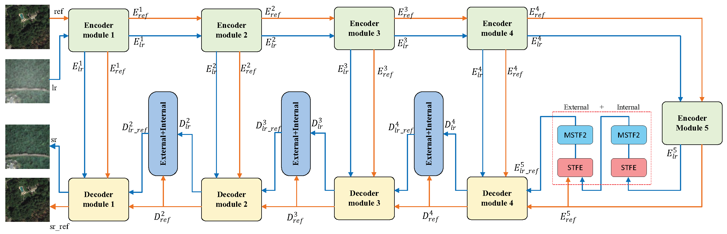
Figure 1 illustrates the overall network architecture of the proposed MSTT-SRNet. We deploy the well-known U-Net architecture as our backbone network. U-Net [35] is widely used in the fields of semantic segmentation and image super-resolution. It is composed of an encoder network (for semantic feature extraction) and a decoder network (for semantic information generation). The peer nodes between the encoder and the decoder are concatenated with each other to integrate semantic information and enhance the generated features. Compared to other backbone networks, U-Net has a relatively symmetrical structure which can well distinguish the low-resolution features from high-resolution features.

Unlike most SR methods, our network has two inputs and two outputs, as shown by the two data flows in Figure 1. The blue data flow indicates that the input is the LR image $I^{lr}$ and the output is the SR image $I^{sr}$. The orange data flow indicates that the input is the Ref image $I^{ref}$ and the output is the SR_Ref image $I^{sr\_ref}$.

In addition, our network combines internal reference and external reference. The input of internal reference is only the LR feature, and the input of external reference includes the LR feature and the Ref feature. These two references both involve two key modules: STFE and MSTF2. The STFE module calculates the similarity relationship between the LR texture feature and the Ref texture feature so as to extract the Ref texture features with high similarity and thus avoid the interference of irrelevant texture features, thereby reducing the complexity of the network. After similar texture feature extraction, the MSTF2 module was designed to transfer the aligned multi-scale Ref texture feature into the LR texture feature. We present the details of these two modules in what follows.

2.2. Similar Texture Feature Extraction Module

Intuitively, common objects from the same class usually share some similarity in texture and have a high similarity in features. To this end, we designed a similar texture feature extraction module to extract the Ref texture features, with high similarity and transferability, which contain the prior knowledge to generate SR results.

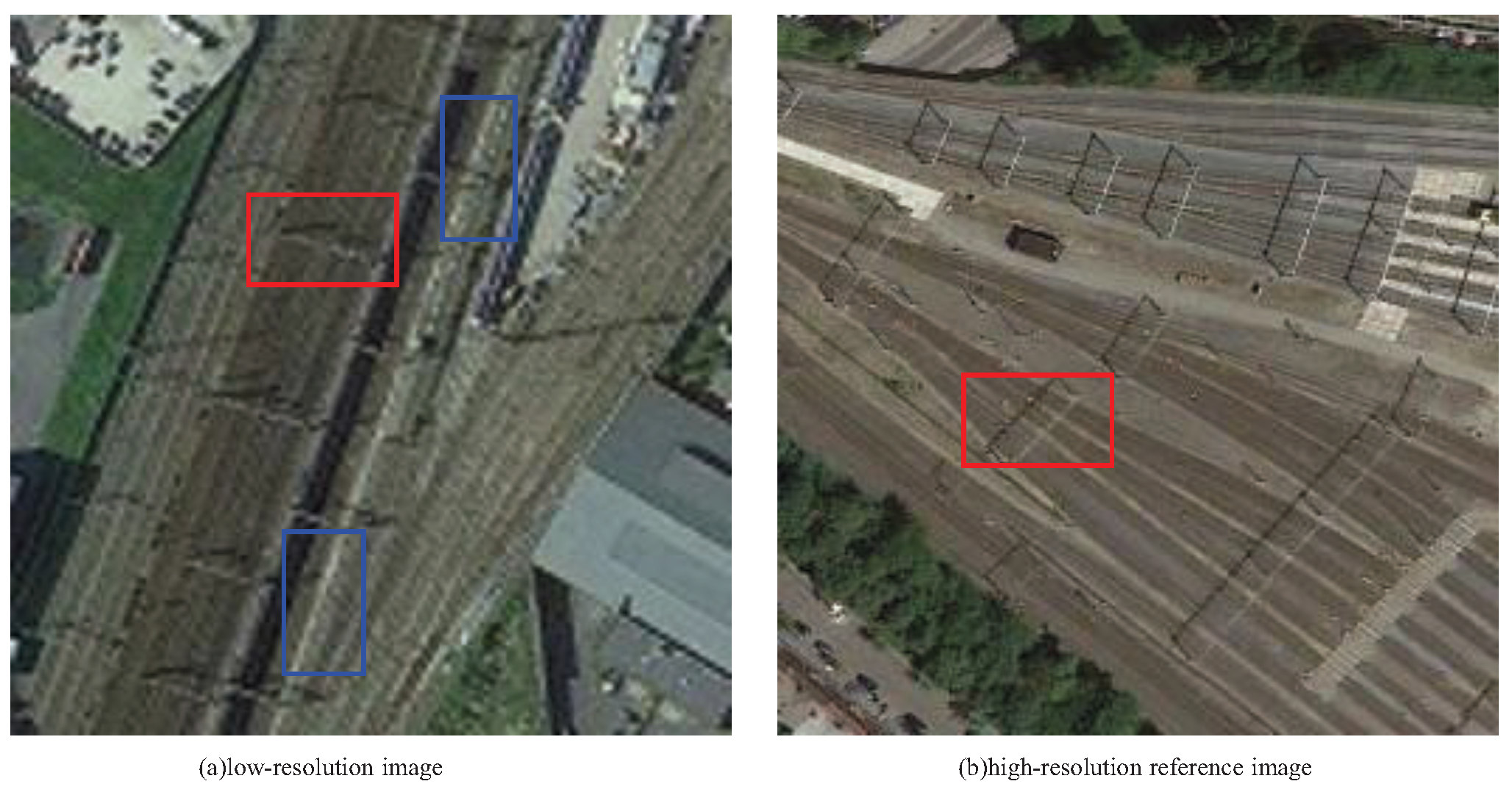
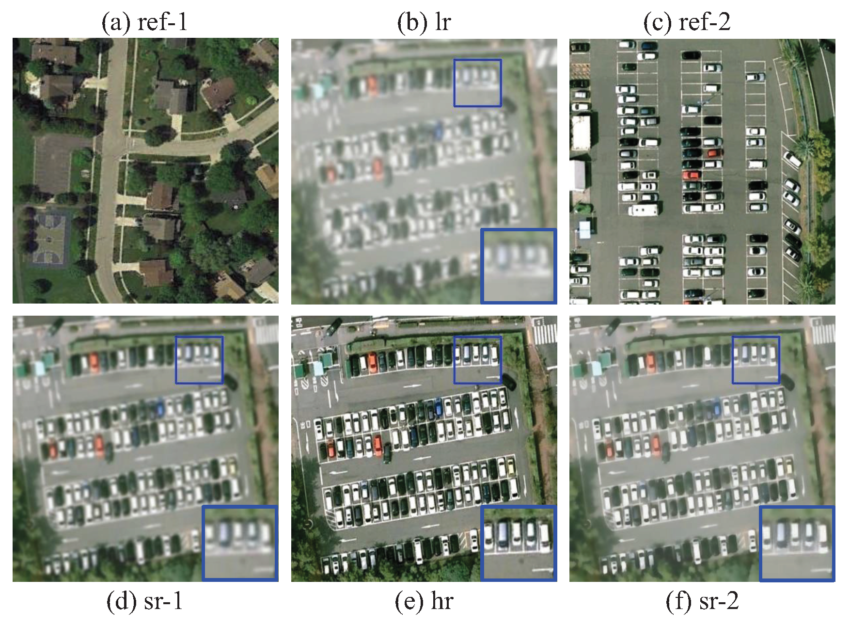
In this paper, the Ref texture features were mainly extracted from two aspects. (1) Internal reference: During the collection of remote sensing images, due to the problems of inappropriate angle, insufficient illumination, and cloud occlusion, the image content may be partially blurred; we can thus extract similar texture features from the image itself. As illustrated in Figure 2, the contents of the two blue boxes are very similar, but the content of the lower blue box is clearer, and thus the latter can be used as the prior knowledge for the content reconstruction of the upper blue box. (2) External reference: If we only rely on internal reference to reconstruct the LR image, the prior knowledge is low-quality and may not contain adequate texture details, limiting the performance in real-world applications. To this end, we leveraged a given high-resolution reference image to provide diverse and rich prior texture knowledge for super-resolution reconstruction, as shown by the two red boxes in Figure 2. The content of the red box in the reference image is very similar to the content of the red box in the low-resolution image, which can help with the content reconstruction.

The combination of internal reference and external reference provides rich and diverse prior knowledge. However, not all prior knowledge is useful for image reconstruction. Irrelevant and redundant texture features can even reduce the effectiveness of reference prior knowledge, making the network too complex to deploy on edge computing devices. The selection and extraction of texture features with high similarity from reference images is essential because accurate and proper texture features assist with the generation of SR images. However, it is challenging to extract such similar and transferable texture features for SR restoration process. Our key idea was to employ the transformer attention mechanism to learn the similarity relationship between LR texture features and Ref texture features, which can guide the extraction of similar texture features. 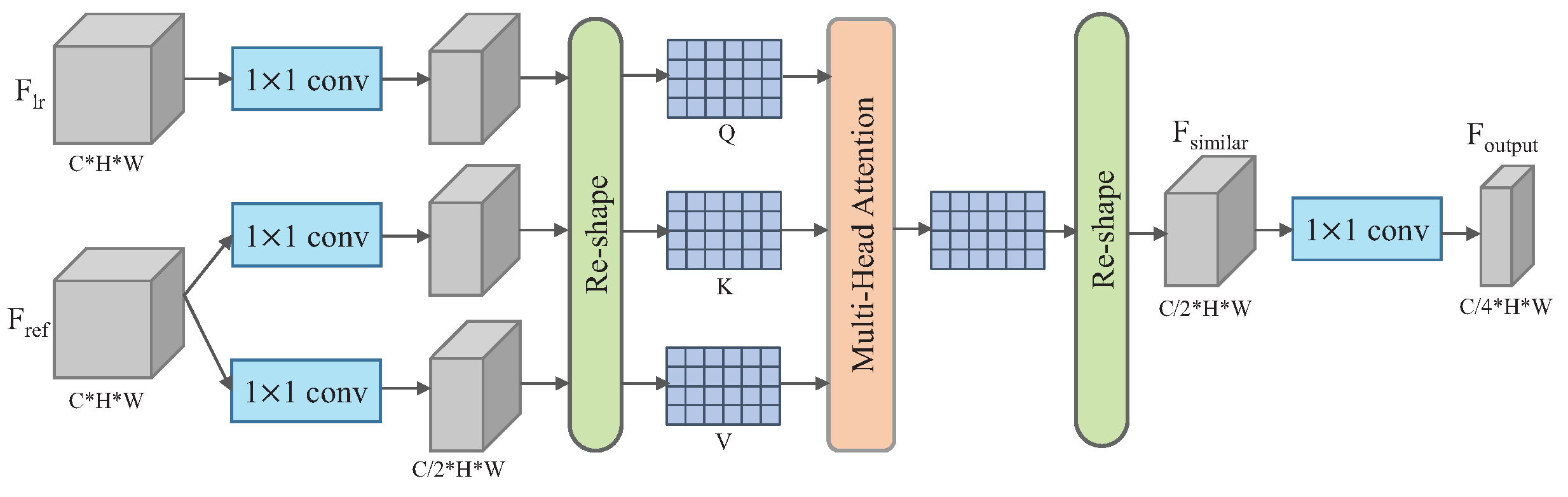Figure 3 illustrates the architecture of the proposed module.

Formally, we denote the LR texture feature as $F_{lr}\in {\mathbb{R}}^{C\times H\times W}$ and the Ref texture feature as $F_{ref}\in {\mathbb{R}}^{C\times H\times W}$, where C, H, and W represent the channel, height, and width of the feature maps, respectively. The transformer attention mechanism uses three learnable linear projection matrices, namely Query Q, Key K, and Value V, to compute the correlation relationship, and extracts the values based on the correlation relationship.

Specifically, in order to reduce the computational complexity and reduce redundant features, we first fed the input features $F_{lr}$ and $F_{ref}$ into different convolution layers to generate feature maps of $F_{lr}^Q$, $F_{ref}^K$, and $F_{ref}^V$. The dimensions of these features were all reduced to $\frac{C}{2}\times H\times W$.

Then, we performed reshape operations on $F_{lr}^Q$, $F_{ref}^K$, and $F_{ref}^V$, and converted the dimension into $HW\times \frac{C}{2}$, respectively. After this, we used these three feature maps to generate the linear projection matrices Q, K, and V to carry out similar texture feature extractions. The process can be formulated as follows:

$$Q=F_{lr}^Q\times W_Q,$$

(1)

$$K=F_{ref}^K\times W_K,$$

(2)

$$V=F_{ref}^V\times W_V,$$

(3)

$$F_{similar}=softmax(\frac{Q{K}^T}{\sqrt{d_k}})V,$$

(4)

where $W_Q$, $W_K$, and $W_V$ are the learnable matrices, respectively. $d_k$ is the normalization factor.

Then, we performed reshape operations on $F_{similar}$, and converted the feature dimension to $\frac{C}{2}\times H\times W$. Finally, we performed feature dimension reduction again to obtain the output Ref texture feature with high similarity, denoted by $F_{output}$; the feature dimension was reduced to $\frac{C}{4}\times H\times W$.

According to different references, in internal reference, $F_{ref}$ is equal to $F_{lr}$. In external reference, $F_{ref}$ is the given reference texture feature. The similar texture feature extraction module enables our model to selectively extract more similar texture features and suppress irrelevant texture features, which can greatly enhance the effectiveness of reference texture features.

2.3. Multi-Scale Texture Feature Fusion Module

After obtaining highly similar Ref texture features, we considered transferring the Ref texture features into the LR texture features to improve the content quality. However, there were two important problems that needed to be solved: one was the texture alignment, the other the texture scale.

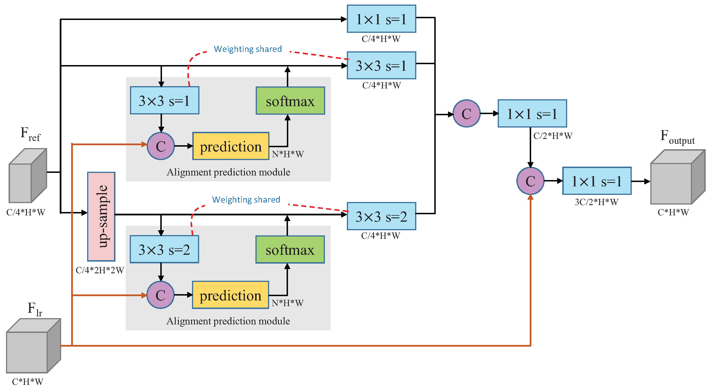
In this section, we propose a novel multi-scale texture feature fusion module for multi-scale Ref texture feature alignment and fusion. As shown in Figure 4, the proposed module adaptively adjusts the texture alignment angles and scales, which can work together to help generate better SR results.

Texture alignment. Since the objects in remote sensing images may appear in any direction and angle, the texture features between the LR image and the Ref image are likely to be misaligned. Therefore, we designed an alignment prediction module to predict the alignment angle for each convolution feature in the Ref features. Specifically, we denote the LR texture feature by $F_{lr}\in {\mathbb{R}}^{C\times H\times W}$ and the Ref texture feature by $F_{ref}\in {\mathbb{R}}^{\frac{C}{4}\times H\times W}$, where C, H, and W represent the channel, height, and width of the feature maps, respectively. We first adopted a $3\times 3$ convolution operation to encode the texture feature, and concatenated it with the LR feature. Then, a $1\times 1\times N$ prediction filter was employed to produce a feature map, with a size of $N\times H\times W$. N represents the alignment angles, which is 8 by default in our paper. Lastly, a softmax function was applied on the feature map to obtain the alignment angles for each feature matrix which will be convoluted in multi-scale texture feature extraction.

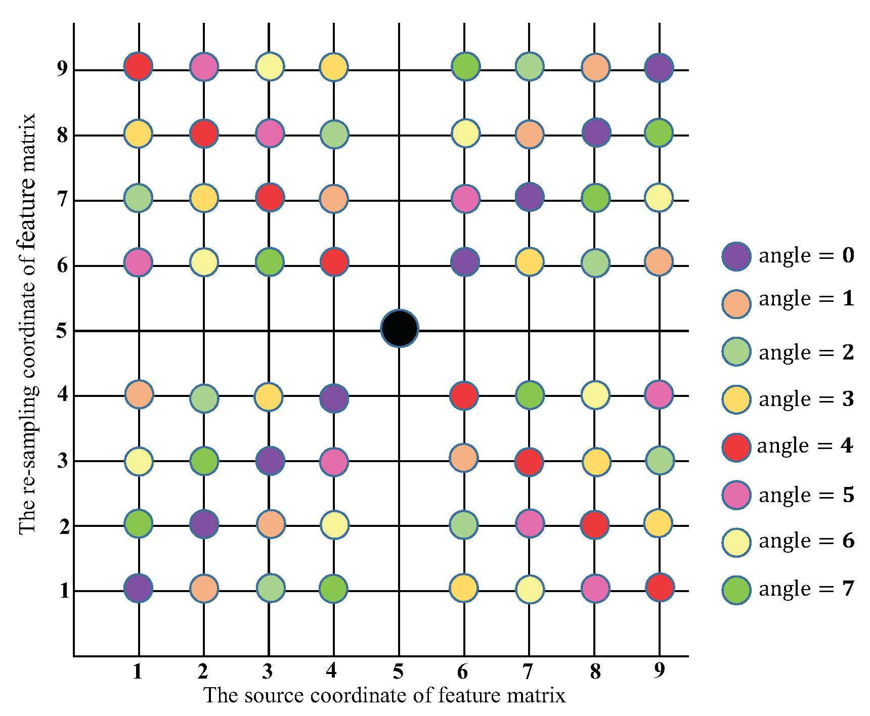
Texture scale. After obtaining the alignment angles, we extracted the multi-scale texture features from three scales. In the first type, we used a $1\times 1$ convolution to extract the Ref texture feature if the scale was equal to the LR texture feature. In the second type, we used a $3\times 3$ convolution with alignment angle to extract the Ref texture feature if the scale was larger than the LR texture feature. In the third type, we first $\times 2$ up-sampled the Ref texture feature by bicubic interpolation, then used a $3\times 3$ convolution with alignment angle to extract the Ref texture feature if the scale was smaller than the LR texture feature, and the stride of the convolution operation was set to 2. The convolution operation with alignment angle is described in the following.

A $3\times 3$ convolution kernel can be expressed as $K=\{k_1,k_2,\dots ,k_n\}$, where n represents the coordinate value in the convolution kernel; it is counted from left to right, then from top to bottom. The maximum value is 9. $k_i$ represents the value of the $i-th$ coordinate point. $F=\{f_1,f_2,\dots ,f_n\}$ represents the corresponding feature matrix which will be convoluted with the $3\times 3$ convolution kernel. A standard 2D convolution operation can be defined as follows:

$$F_{output}=(F\ast K)\left(n\right)={\displaystyle \sum _{i=1}^n}\left(f_i{k}_i\right)$$

(5)

In our study, we needed to rotate the texture feature F before the convolution operation according to the predicted alignment angle to re-sample a new texture feature matrix $\widehat{F}=\{\widehat{f_1},\widehat{f_2},\dots ,\widehat{f_n\}}$. The re-sampling locations of different alignment angles are shown in Figure 5.

In this way, we were able to align the Ref texture feature to the LR texture feature. The new convolution operation can be defined as follows:

$$\widehat{F_{output}}=(\widehat{F}\ast K)\left(n\right)={\displaystyle \sum _{i=1}^n}\left(\widehat{f_i}{k}_i\right)$$

(6)

Then, the aligned multi-scale Ref texture features were concatenated, and fused by a $1\times 1$ convolution operation.

Finally, based on the aligned multi-scale Ref texture feature, a fusion operation was conducted to transfer the Ref texture feature into the LR texture feature, which was then used as the SR feature to generate the SR image.

2.4. Loss Function

In order to obtain better SR results, we used the weighted sum of multiple loss components to calculate the total loss function. The total loss function is defined as follows:

$${\mathcal{L}}_{total}={\lambda }_{cont}{\mathcal{L}}_{cont}+{\lambda }_{per}{\mathcal{L}}_{per}+{\lambda }_{text}{\mathcal{L}}_{text}$$

(7)

where ${\mathcal{L}}_{cont}$ denotes the content loss, ${\mathcal{L}}_{per}$ denotes the perception loss, ${\mathcal{L}}_{text}$ denotes the texture transfer loss, and ${\lambda }_{rec}$, ${\lambda }_{per}$, and ${\lambda }_{text}$ are the balancing weights.

Content loss. The content loss consists of two parts: one is the content loss of the input LR image, and the other is the content loss of the Ref image. We used $L1$ loss to measure the content loss, which was demonstrated better than $L2$ loss and supported easier convergence. The calculation formula is defined as follows:

$${\mathcal{L}}_{cont}=\frac{1}{CHW}{∥I^{sr}-I^{hr}∥}_1+\frac{1}{CHW}{∥I^{sr-ref}-I^{ref}∥}_1$$

(8)

where $I^{sr}$ and $I^{hr}$ denote the reconstructed image and the ground-truth high-resolution image of the input low-resolution image, respectively. $I^{sr-ref}$ and $I^{ref}$ denote the reconstructed reference image and the input high-resolution reference image, respectively. C, H, and W represent the channel, height, and width of the images, respectively.

Perception loss. The content loss was too rigid to measure the content difference by pixel-to-pixel value. Perception loss measures the content difference through high-dimensional semantic features which are closer to the results of human perception. We measured the perception loss through the feature maps extracted by the VGG-19 network. The perception loss also includes two parts: one is the perception loss of the LR image, and the other is the perception loss of the Ref image. The formula is defined as follows:

$${\mathcal{L}}_{per}=\frac{1}{CHW}{∥{\varphi }_i\left(I^{sr}\right)-{\varphi }_i\left(I^{hr}\right)∥}_1+\frac{1}{CHW}{∥{\varphi }_i\left(I^{sr-ref}\right)-{\varphi }_i\left(I^{ref}\right)∥}_1$$

(9)

where $\varphi (·)$ denotes the VGG-19 network, and i represents the i-th layer’s feature map of the VGG-19 network. In this paper, we simply adopted the relu5_1 layer’s feature map. C, H, and W represent the channel, height, and width of the feature map, respectively.

Texture transfer loss. As the content loss and perception loss cannot guarantee that the texture of the SR image is transferred from the Ref image, we introduced a texture transfer loss to enhance the effectiveness of the texture transfer. With our texture transfer loss we attempted to restrict the SR texture feature so that it would be close to the Ref texture feature. We adopted the cosine similarity calculation to measure the texture similarity between the SR texture feature and the Ref texture feature. The texture transfer loss is defined as follows:

$${\mathcal{L}}_{text}={\displaystyle \sum _{j=0}^3}(1-cos(F_j^{sr},F_j^{ref}))$$

(10)

where j denotes the number of the External+Internal module. $cos(·)$ represents the cosine function, the value range is normalized from 0 to 1, and the high value indicates the high similarity. $F_j^{sr}$ denotes the output SR feature of external reference. $F_j^{ref}$ denotes the Ref texture feature which was fed into the external reference.

3. Experimental Results

In this section, we first describe the construction process of the dataset used in this paper and provide the implementation details. Then, we evaluate the performance of our method compared with other SR methods. Then, we fully verify the effectiveness of our designed modules by ablation experiments. Lastly, we test the application effect of our proposed method in smart cities by the task of urban region function recognition.

3.1. Datasets

Since there are no open available datasets for remote sensing images super-resolution with reference images, we chose the AID dataset [36] and WHU-RS19 dataset [37] to construct the training set and test set. These two datasets have relatively high pixel and spatial resolution.

The AID dataset was released by the Huazhong University of Science and Technology and Wuhan University in 2017. It contains 30 classes, with about 220–420 remote sensing images in each class. The total number is 10,000. The pixel resolution is $600\times 600$, and the spatial resolution is 0.5 m∼8 m.

The WHU-RS19 dataset was released by Wuhan University in 2011. It contains 19 classes. Each class has about 50 images with $600\times 600$ pixels. The spatial resolution is 0.5 m. The total number is 1005.

Considering that the similarity between the LR image and the Ref image affects the super-resolution results significantly, we regarded the former image as the original HR image and the latter image as the corresponding Ref image in the same class. This strategy can ensure that the original HR image and the Ref image have a high texture similarity. In this way, we collected 5500 HR–Ref pair samples.

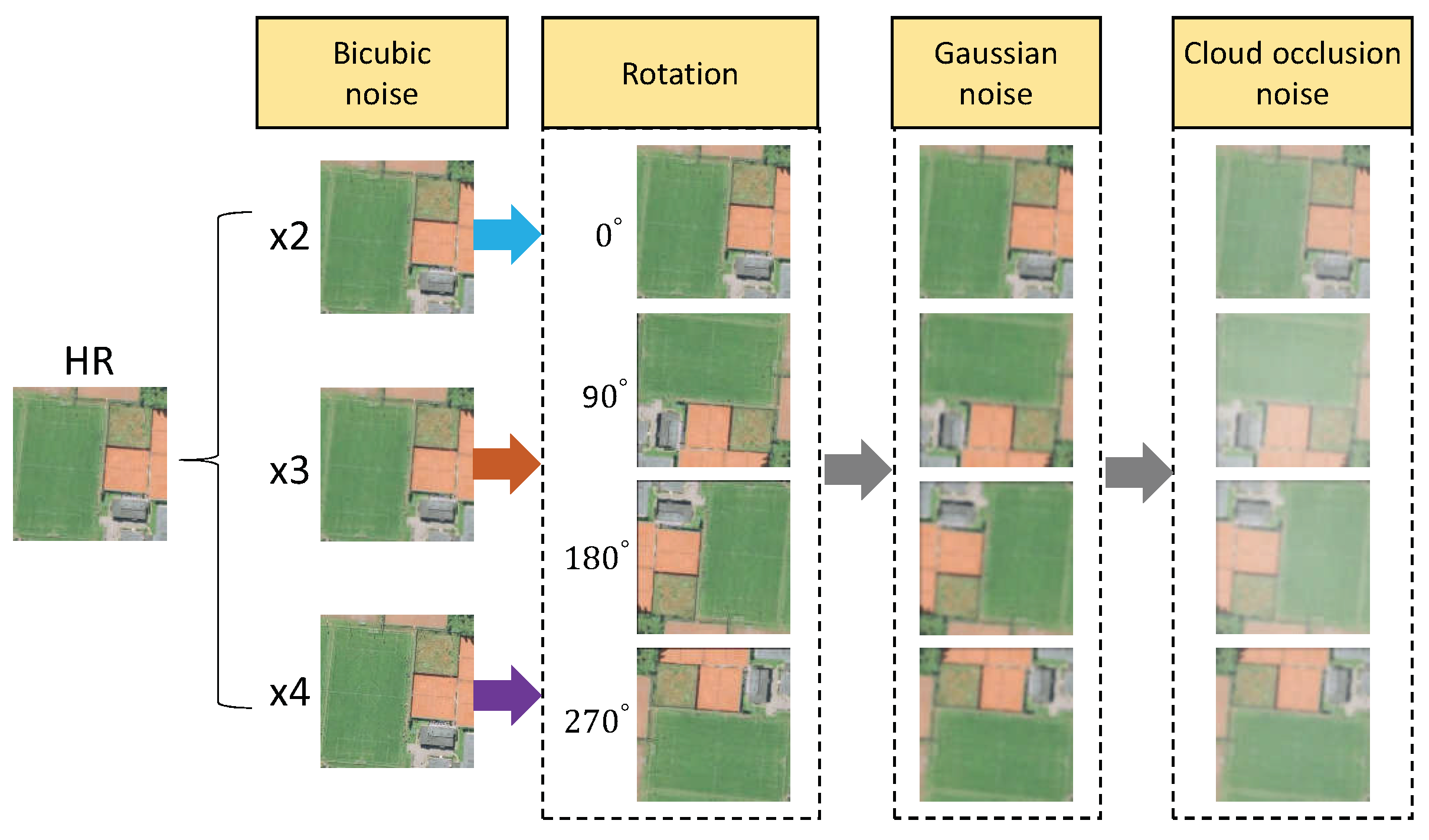
Figure 6 shows the image degradation process in our paper.

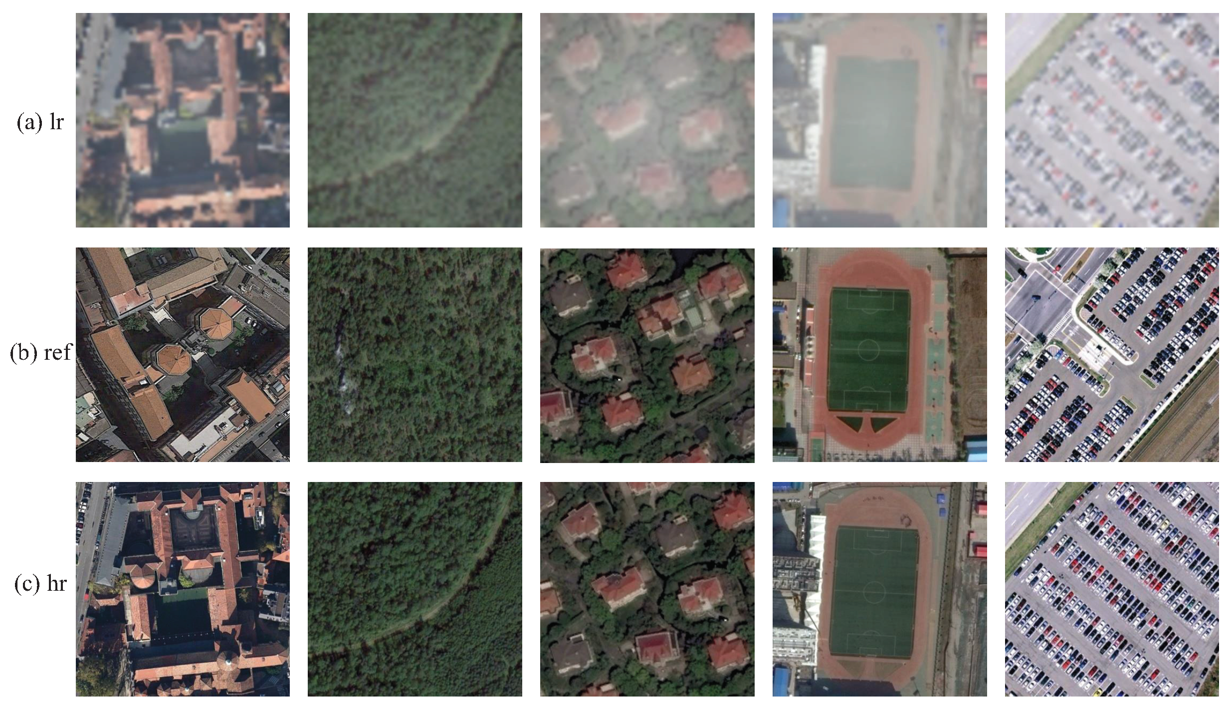
Finally, we obtained 22,000 pair samples in every scaling factor. Each pair sample included a low-resolution image, a reference image, and a high-resolution ground truth image. We selected 20,000 samples for training and 2000 samples for testing. Figure 7 shows some examples in the dataset.

3.2. Metrics

In this paper, we chose two standard evaluation metrics, peak signal-to-noise ration ($PSNR$) and the structural similarity index measure ($SSIM$) [38], as the objective measure indexes to evaluate the performance of our method and other compared SR methods.

We calculated the $PSNR$ as follows:

$$MSE=\frac{1}{mn}{\displaystyle \sum _{i=0}^{m-1}}{\displaystyle \sum _{j=0}^{n-1}}{[X(i,j)-Y(i,j)]}^2,$$

(11)

$$PSNR=10·{log}_{10}(\frac{MA{X}_X^2}{MSE}),$$

(12)

where X denotes the HR image, Y denotes the SR image, $m\times n$ represents the pixel resolution of the image, and $MAX$ denotes the maximum possible pixel value of the image, which was set to 255 in our experiments.

$SSIM$ was calculated from three aspects: brightness, contrast, and structure. The value ranged from 0 to 1. The larger the value, the more similar the structure.

Brightness was calculated by mean as follows:

$$l(X,Y)=\frac{2{\mu }_X{\mu }_Y+c_1}{{\mu }_X^2+{\mu }_Y^2+c_1},$$

(13)

Contrast was calculated by variance as follows:

$$c(X,Y)=\frac{2{\sigma }_X{\sigma }_Y+c_2}{{\sigma }_X^2+{\sigma }_Y^2+c_2},$$

(14)

Structure was calculated by covariance as follows:

$$s(X,Y)=\frac{{\sigma }_{XY}+c_3}{{\sigma }_X{\sigma }_Y+c_3},$$

(15)

where ${\mu }_X$ and ${\mu }_Y$ represent the mean value, ${\sigma }_X$ and ${\sigma }_Y$ represent the standard deviations, and ${\sigma }_{XY}$ denotes the cross-covariance. $c_1={\left(k_{1}L\right)}^2$ and $c_2={\left(k_{2}L\right)}^2$ are two constants to avoid division by zero, where L is set to 255, and $k_1$ and $k_2$ are set to 0.01 and 0.03, respectively, in our experiments.

$SSIM$ can be calculated as follows:

$$SSIM(X,Y)=[l{(X,Y)}^{\alpha }·c{(X,Y)}^{\beta }·s{(X,Y)}^{\gamma }],$$

(16)

Now, with $\alpha =1$, $\beta =1$, $\gamma =1$, and $c_3=\frac{c_2}{2}$, the formula can be changed to:

$$SSIM(X,Y)=\frac{(2{\mu }_X{\mu }_Y+c_1)(2{\sigma }_{XY}+c_2)}{({\mu }_X^2+{\mu }_Y^2+c_1)({\sigma }_X^2+{\sigma }_Y^2+c_2)}.$$

(17)

3.3. Implementation

While training the MSTT-SRNet, the batch size was set to 4. We used Adam [39] as the optimizer with a weight decay of $5\times {10}^{-4}$. We trained the network for 25 epochs. The initial earning rate was 0.001 and it decreased by a factor of 10 every 10 epochs. The multi-head in the transformer was set to 8. The weights of ${\lambda }_{cont}$, ${\lambda }_{per}$, and ${\lambda }_{text}$ were 5.0, 1.0, and 1.0, respectively. Our proposed method was implemented by PyTorch, and all the experiments were run on a NVIDIA Titan XP GPU (12GB memory).

3.4. Comparisons with State-of-the-Art Methods

In order to better demonstrate the effectiveness of our method, we compared our method with several other SR methods. The compared methods were bicubic, FSRCNN [14], EDSR [19], TTSR [31], and DASR [25]. Bicubic is a typical traditional interpolation method. FSRCNN and EDSR are traditional non-blind super-resolution methods. TTSR is also a reference-based super-resolution method. DASR is a blind super-resolution method.

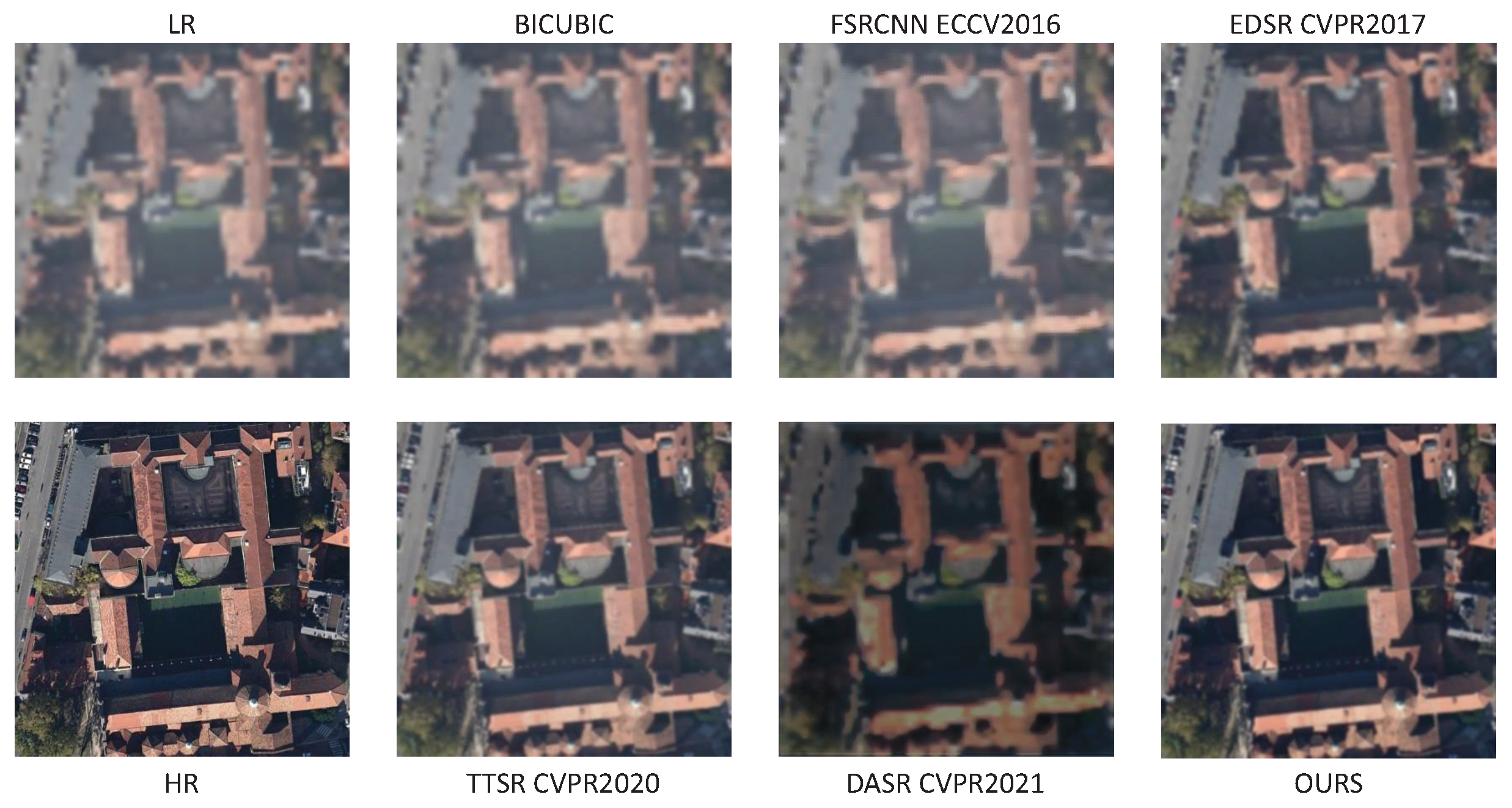
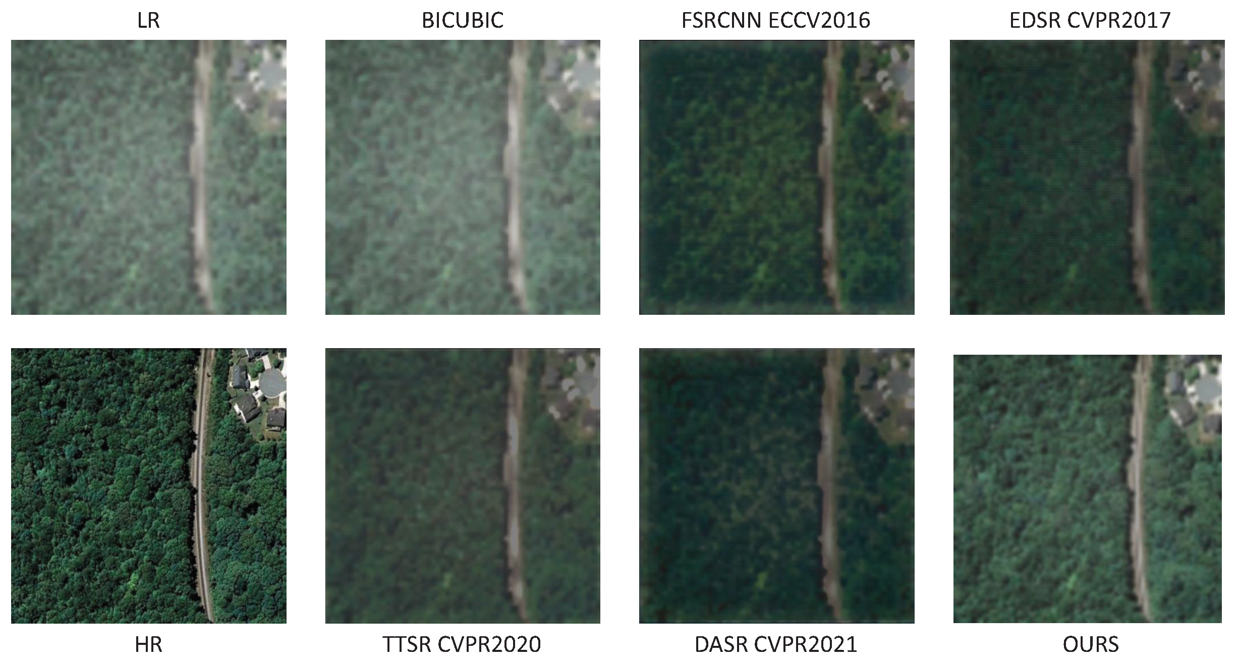
Figure 8 and Figure 9 show the visual reconstruction effect of scaling factors $\times 2$ and $\times 4$, respectively. We can see that: (1) the images reconstructed by the bicubic method are very blurry, the detail information is missing, and the visual effectiveness is poor; (2) the images reconstructed by the FSRCNN method and the EDSR method demonstrate a great improvement in the content details, but there are still many cases where the boundary lines are blurred, and the reconstruction effect is not ideal; (3) The images reconstructed by the DASR method have a certain distortion, especially in the second group of samples, and color distortion occurs, the main reason being that the estimation of the image degradation type by this method does not deal with the degradation problem of cloud occlusion; (4) TTSR is also a reconstruction method based on texture reference, but the effect on remote sensing images is not ideal. The reason may be that the method is based on correlation analysis between low-resolution image features and the same down-sampled reference image features. However, there is no cloud occlusion degradation in the reference image, which affects the correlation learning between low-resolution features and reference features; (5) Our method learns the texture correlation between the reconstruct features and the reference features in the decoder stage, both of which have no cloud occlusion noise. Therefore, compared with other methods, the method proposed in this paper results in the best reconstruction effect, and the texture details are more abundant, which fully verifies the effectiveness of the method.

To further analyze the objective performance of our method, we reported the mean $PSNR$ and $SSIM$ values compared with other methods on test sets of various scaling factors.

Table 1. The mean $PSNR$(dB) and $SSIM$ on a test set with scale factors of $\times 2$, $\times 3$, and $\times 4$.

	Scale	Bicubic	FSRCNN	EDSR	TTSR	DASR	Ours
$PSNR$/dB	$\times 2$	29.71	31.64	31.86	31.94	30.83	32.31
	$\times 3$	27.39	28.21	28.55	29.03	28.87	29.86
	$\times 4$	25.42	26.91	27.01	27.22	26.33	27.65
$SSIM$	$\times 2$	0.895	0.902	0.904	0.913	0.899	0.918
	$\times 3$	0.812	0.845	0.841	0.856	0.854	0.866
	$\times 4$	0.781	0.803	0.811	0.812	0.806	0.831

shows the statistical results. It can be seen from the table that our method achieves better results than other state-of-the-art methods, which demonstrates the effectiveness of our method.

3.5. Analysis of Different Reference Images

In order to better analyze the reconstruction effectiveness as affected by different Ref images, Figure 10 shows the comparison of the generated SR results based on different Ref images. It can be seen from the figure that the texture similarity between the LR image and the Ref image on the left is low and that the SR result is poor, while the Ref image on the right has a high texture similarity with the LR image and the texture details of the corresponding SR result are richer, which fully indicates that it is effective for adopting a Ref image to help with SR reconstruction. At the same time, the Ref image with higher texture similarity has a higher reference value for helping with SR reconstruction.

3.6. Ablation Studies

In this section, we conduct several ablation experiments to verify the effectiveness of the key components in our method, including the similar texture feature extraction module, the multi-scale texture feature fusion module, and the texture transfer loss.

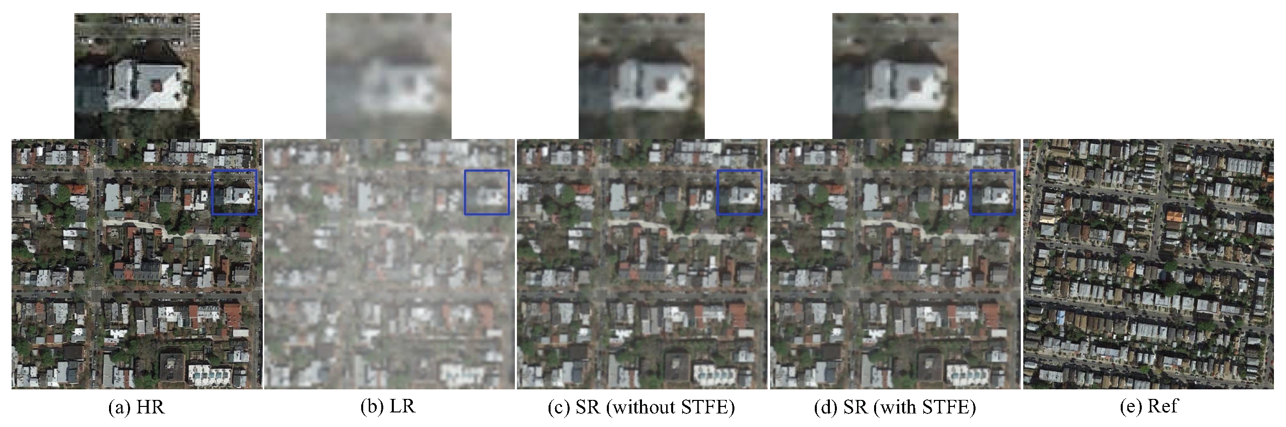
Similar texture feature extraction module. The function of the similar texture feature extraction module (STFE) lies in using a transformer attention mechanism to extract the high similarity texture feature from the Ref image, and in doing so to avoid the interference of irrelevant and redundant texture features to obtain more valuable reference prior knowledge.

To verify the effectiveness of the STFE module, we designed an ablation experiment. We removed the STFE module from the full model. For fairness, we also performed a $1\times 1$ convolution operation on the Ref texture feature to reduce the feature dimension. Then, we fed the Ref texture feature to the MSTF2 module for the SR task.

Figure 11 shows the visual comparison results of scaling factor $\times 2$. We can see that both the LR image and the Ref image contain many objects, and the texture information is complex. Although they have a high texture similarity, the SR result from the network without STFE is poor, while the network with STFE restores richer texture details and a more realistic SR result, demonstrating the superior usefulness of the STFE module in the selection and extraction of Ref texture features.

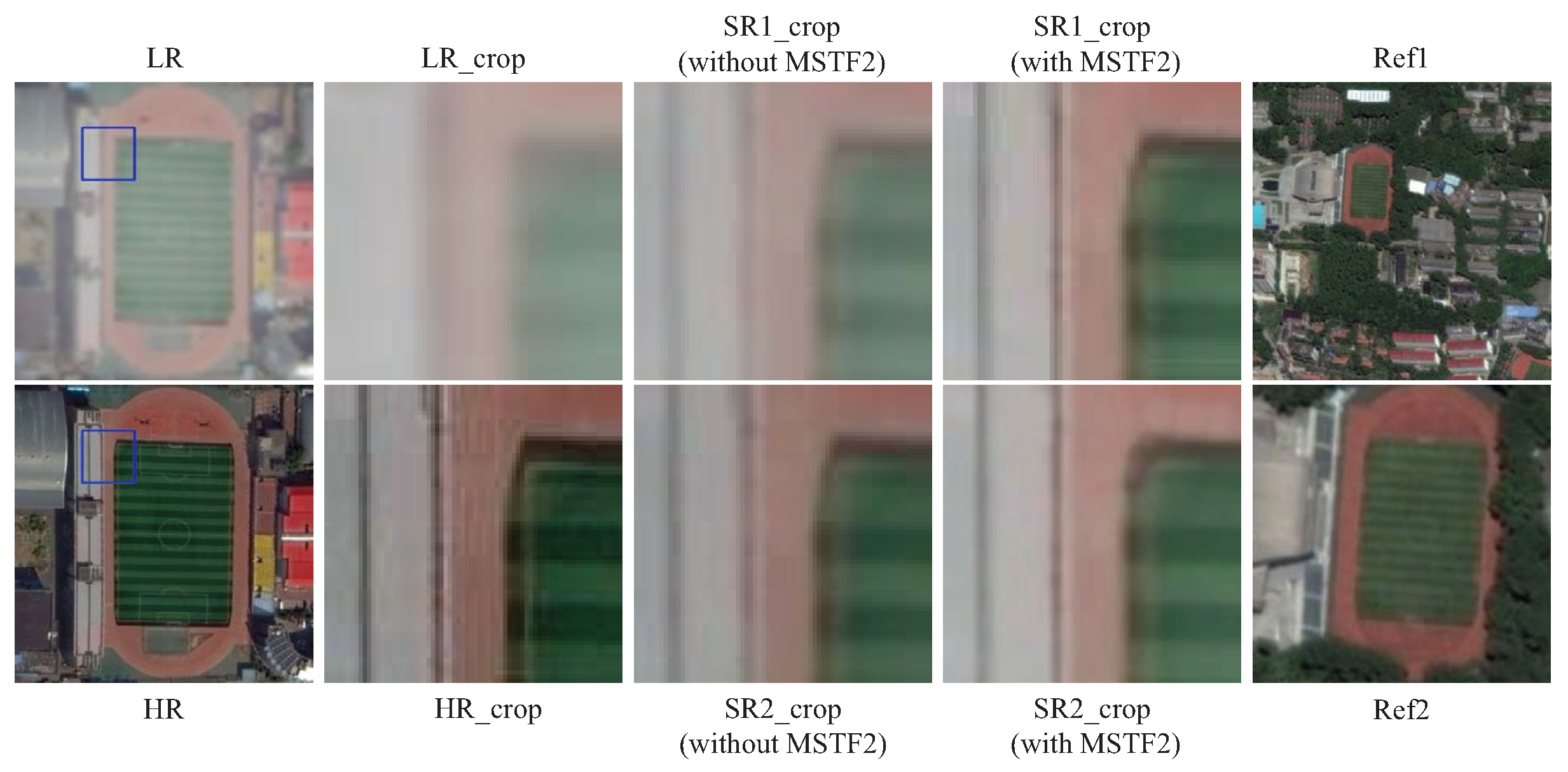
Multi-scale texture feature fusion module. To study the effect of the MSTF2 module, we conducted an experiment by removing the MSTF2 module from the full model, then compared the SR results with those from the full model. In addition, we also conducted an experiment by cutting the playground area from the Ref image and then up-sampling by bicubic interpolation to $600\times 600$ as the new Ref image, which means the different scales of the Ref images, though the experiment is not fully comparable. We show the performance comparison results of these two models based on differently scaled Ref images in Figure 12. As shown in the figure, under the same scale of the Ref image, the model with the MSTF2 module could obtain better SR results compared with the model without the MSTF2 module, which demonstrates the effectiveness of the proposed MSTF2 module. Under the different scales of Ref images, the results of the model without the MSTF2 module are superior when the scale of the Ref image is large, which implies that texture scale matters. By adding the MSTF2 module, the SR results of different scales are relatively approximate. This demonstrates the stronger adaptivity of multi-scale in extracting Ref texture features.

Texture transfer loss. To ensure that the texture transfer loss would benefit our network, we trained the MSTT-SRNet twice. The first training did not include texture transfer loss, while the second training did.

Table 2. The compared mean $PSNR$(dB) and $SSIM$ on a test set trained by MSTT-SRNet without and with texture transfer loss with scale factors of $\times 2$, $\times 3$, and $\times 4$.

Scaling Factor	Texture Transfer Loss	$\mathbf{PSNR}$/dB	$\mathbf{SSIM}$
$\times 2$	without	31.81	0.911
	with	32.31	0.918
$\times 3$	without	29.37	0.857
	with	29.86	0.866
$\times 4$	without	27.31	0.819
	with	27.65	0.831

shows the quantitative comparison results of these two training networks with various scaling factors. We can see that: (1) in the scaling factor $\times 2$, texture transfer loss provides a 0.5 dB improvement in $PSNR$, and a 0.007 improvement in $SSIM$; (2) in the scaling factor $\times 3$, texture transfer loss provides a 0.49 dB improvement in $PSNR$, and a 0.009 improvement in $SSIM$; (3) in the scaling factor $\times 4$, texture transfer loss provides a 0.34 dB improvement in $PSNR$, and a 0.012 improvement in $SSIM$. The above results show the effectiveness of texture transfer loss.

3.7. Application in Smart Cities

In this section, we evaluate the application effect of our proposed SR method in smart cities. We applied our SR method to a challenging large-scale dataset for urban region function recognition (URFR dataset). The dataset was released by the 5th Baidu and XJTU Big Data Contest in 2019. The aim of the contest was to design an urban region function classification model based on remote sensing images and user visit data. The dataset consists of two parts: the first part was provided in the preliminary round, denoted as URFR-1, and includes 40,000 training samples and 10,000 test samples. The second part was provided in the semi-final round, denoted as URFR-2, and included 400,000 training samples and 100,000 test samples. There were nine types of region function labels in the dataset, namely residential area (res.), school (sch.), industrial park (ind.), railway station (rail.), airport (air.), park (park), shopping area (shop.), administrative district (adm.), and hospital (hosp.). In our experiments, we only used the remote sensing images in the training samples with ground truth labels. This dataset was particularly challenging as the resolution of the remote sensing images was $100\times 100$, and the image content was blurry. Some images even had serious cloud occlusion, which led to poor performance based on this dataset.

Table 3. The split settings and per-class numbers of the URFR-1 and URFR-2 datasets.

Dataset	Split	res.	sch.	ind.	rail.	air.	park	shop.	adm.	hosp.	Total
URFR-1	train	8152	6417	3031	1155	2947	4685	2973	2209	2431	34,000
	val	217	188	98	40	85	140	87	68	77	1000
	test	1173	933	461	163	432	682	457	340	359	5000
URFR-2	train	102,211	77,520	43,315	5592	14,000	53,300	17,987	11,191	14,884	340,000
	val	3094	2201	1338	170	410	1558	514	321	394	10,000
	test	15,065	11,332	6362	826	2084	7826	2634	1669	2202	50,000

shows the details of the URFR-1 and URFR-2 datasets.

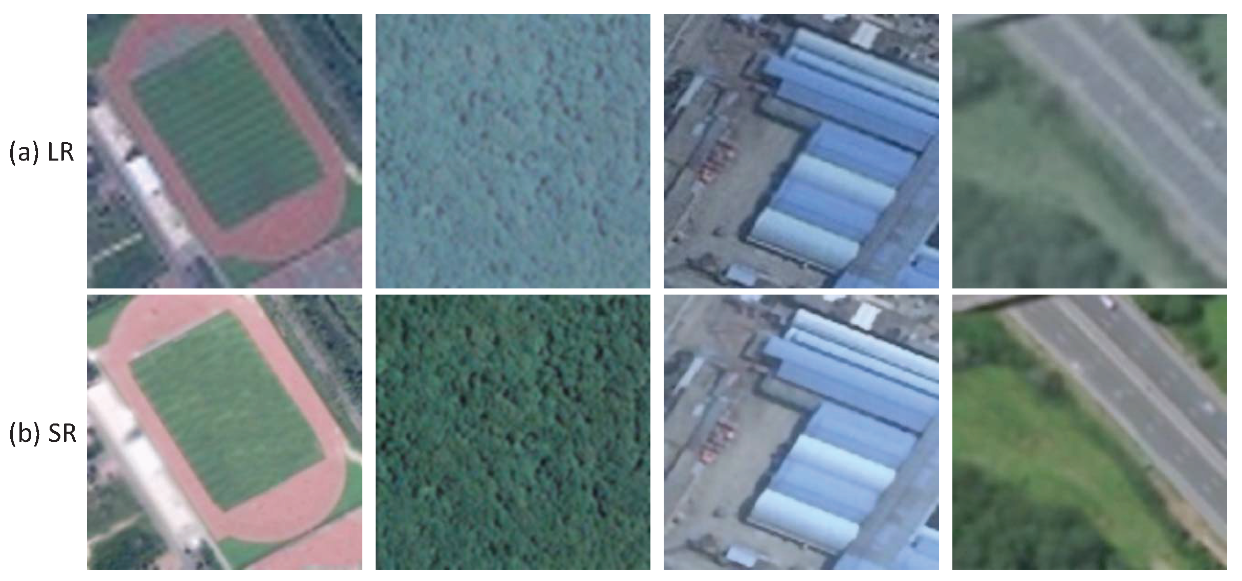
Visual Comparison. Figure 13 shows some remote sensing images in the URFR dataset and the corresponding SR results generated by our proposed method. From the visual comparisons, we can see that the SR results reconstructed by our proposed method have clearer edges and richer textures.

Quantitative Evaluation. We performed the urban region function recognition experiments on three widely used convolutional neural networks, namely VGG-19 [40], ResNet-50 [41], and DenseNet-121 [42], to evaluate the application effect. We conducted a comparative experiment. (1) Before SR: We used the original URFR dataset to train in turn the three classification networks pre-trained on ImageNet. (2) After SR: We applied our proposed SR method to the URFR dataset to generate the SR images. Then, we used the SR URFR dataset to train in turn the three classification networks pre-trained on ImageNet again. In our experiment, we set the same training parameters to the same type of classification network during the two comparative training processes. We adopted the SR results of scaling factor $\times 3$. We resized both the original images and the SR images to $224\times 224$ for training and testing.

Table 4. The accuracy results of the comparative experiments on the URFR-1 and URFR-2 test sets.

Network	Image Type	Accuracy (URFR-1 %)	Accuracy (URFR-2 %)
VGG-19	original images	39.81	53.82
	SR images	42.13	56.34
ResNet-50	original images	44.48	54.72
	SR images	48.59	58.50
DenseNet-121	original images	45.08	55.43
	SR images	49.12	59.84

summarizes the accuracy results of the comparative experiments on the URFR-1 and URFR-2 test sets. From the results, we can see that the accuracy results after SR of the three classification networks all outperformed the results before SR. The accuracy of VGG-19, ResNet-50, and DenseNet-121 on the URFR-1 test set were improved by 2.32%, 4.11%, and 4.04%, respectively. The accuracy of VGG-19, ResNet-50, and DenseNet-121 on the URFR-2 test set were improved by 2.52%, 3.78%, and 4.41%, respectively. This indicates that our proposed SR method can effectively improve remote sensing image quality and enhance the application value in smart-city-related tasks.

4. Discussion and Conclusions

In this paper, to address the problems of insufficient resolution and blurry content of remote sensing images, we proposed a novel SR method, called the multi-scale texture transfer super-resolution network (MSTT-SRNet), which effectively leverages internal and external reference prior knowledge. Particularly, the proposed method introduces the transformer attention mechanism in order to exploit the texture similarity measurement between the LR image and the Ref image to enhance the transfer texture feature representation and reduce the parameters and computation of the network. At the same time, considering the diverse scales and alignment angles of texture features, a multi-scale texture feature fusion module was designed to obtain more accurate reconstruction results. The experimental results show that our proposed method can achieve better subjective and objective performance compared with several state-of-the-art SR methods.

In addition, we also evaluated the application value of our proposed SR method in smart cities through the task of urban region function recognition. The dataset used in this task was particularly challenging as the resolution of the remote sensing images was very low ($100\times 100$) and the image content was blurry; some images even had serious cloud occlusion, which led to poor performance. We applied our proposed SR method to this low-quality dataset. We then conducted comparative experiments between the SR dataset and the original dataset on three widely used convolutional neural networks: VGG-19, ResNet-50, and DenseNet-121. The results show that our proposed SR method can effectively increase the accuracy of urban region function recognition. This indicates that our proposed SR method has high application value in smart cities.

However, we found some problems during the experiment. Compared with real-world datasets, the synthetic dataset in our paper based on the AID and WHU-RS19 datasets did not contain sufficient variant scales. Thus, the texture scale difference between LR and Ref images was small, which led to inadequate learning in the extraction and fusion of multi-scale texture features. In the future, we will explore the variant scales in the process of dataset construction. The possible ways to do this include choosing source datasets with different spatial resolutions and selecting LR–Ref pair samples with scale variation. Moreover, we also need to further test the application effect of our proposed method in more smart city tasks based on remote sensing images.