Enhancement of the HILOMOT Algorithm with Modified EM and Modified PSO Algorithms for Nonlinear Systems Identification

Abstract

Developing a mathematical model has become an inevitable need in studies of all disciplines. With advancements in technology, there is an emerging need to develop complex mathematical models. System identification is a popular way of constructing mathematical models of highly complex processes when an analytical model is not feasible. One of the many model architectures of system identification is to utilize a Local Model Network (LMN). Hierarchical Local Model Tree (HILOMOT) is an iterative LMN training algorithm that uses the axis-oblique split method to divide the input space hierarchically. The split positions of the local models directly influence the accuracy of the entire model. However, finding the best split positions of the local models presents a nonlinear optimization problem. This paper presents an optimized HILOMOT algorithm with enhanced Expectation–Maximization (EM) and Particle Swarm Optimization (PSO) algorithms which includes the normalization parameter and utilizes the reduced-parameter vector. Finally, the performance of the improved HILOMOT algorithm is compared with the existing algorithm by modeling the $N{O}_x$ emission model of a gas turbine and multiple nonlinear test functions of different orders and structures.

1. Introduction

With modern advancements in engineering there is an emerging need to develop well-formulated models. Models have significance in all disciplines of studies. Models help to understand the behavior of a system when it is not feasible to run experiments on a real system. This knowledge can be further employed for numerous purposes, such as simulation, prediction, controller design, fault detection etc. However, modern automated systems are incredibly involved and recondite; hence, the complexity of systems is escalating progressively with time. Thus, finding an analytical model can become tedious or hectic. In such cases, an experimental modeling approach also known as system identification is employed. System identification approximates a relationship between the system’s input and output based on its input and output data. System identification can be classified into linear system identification and nonlinear system identification based on the type of system. Since most practical systems demonstrate nonlinear characteristics, a noteworthy effort is concentrated towards modeling nonlinear systems.

Linear models can approximately represent systems that exhibit weak nonlinearities [1]. Instances where linear models are applied can be found in [2,3,4,5,6,7,8]. However, the performance of these models is substantially reduced when a system features strong nonlinearities [1,9,10]. Although some works have achieved curtailment of these effects by linearizing a nonlinear system about a point of interest, the effectiveness of these models degrades for processes with a wide range of operation and strong nonlinearities [11]. The opportunity cost between the nonlinear model and the linear model is accuracy and complexity [1] (p. 1).

On the other hand, nonlinear identification is employed for highly nonlinear systems. Nonlinear systems modeling presents many challenges due to their diversity in structure, which requires the modeling algorithm to be universal to represent a wide range of systems [12]. Several architectures such as block-oriented [13,14,15,16,17,18], Volterra series [19], and polynomial Nonlinear Auto-regressive Network with Exogenous Inputs (NARXs) [20,21,22,23] can be found in the literature. Although these models have demonstrated effectiveness in numerous diverse scenarios, they have limitations. Notably, the nonlinear structures of these models are rigid to some extent, thus requiring prior knowledge about the system structure. Furthermore, black-box models, for instance, wavelet [24,25], neural networks [26,27,28,29,30], and support vector machines [31,32,33], have also been employed, which lack interpretability and suffer from the curse of dimensionality [34]. Furthermore, due to the lack of transparency of the models, they are not very useful for model-based control system design. A comprehensive study on nonlinear system identification can be found in [35,36].

Another approach to identify and model intricate nonlinear systems is the Multi-Model Framework (MMF) [37,38,39,40,41]. MMF has appeared in variety of contexts, such as regime-based multi-model [42], Piece-Wise Continuous (PWC) systems [43], Local Radial Basis Function Networks (LRBFNs) [44], Takagi–Sugeno (T–S) fuzzy local model [45], and Local Model Networks (LMNs) [46]. Despite constructing input-dependent and less accurate models [47] (p. 29), MMF has been exploited to model systems in several disciplines [48,49,50,51,52,53,54,55,56]. MMF dissolves the entire input space into smaller sub-regions, defined by validity functions, which hold the local models [57]. These local models can have various structures [57]; however, local linear models are essential for controller design because they allow for the transfer of the mature linear control theory to the nonlinear paradigm [58]. Furthermore, with local linear models, there is a fair compromise between the number of required local models and the complexity of the local models [59].

The advantage of the MMF approach relies on the possibility of incorporating specific knowledge about a system by decomposing the entire input space into multiple sub-regions that hold the local models. The local models depict the dynamic of the process in each of these regions. Hence, partitioning the sub-regions is an essential step in determining the model’s efficacy [57].

HILOMOT [59] is an iterative algorithm that uses axis-oblique splitting to hierarchically split the entire input premise. HILOMOT, which is the advancement of the popular LOLIMOT [44] algorithm, is inspired by the Hinging Hyper-plane Trees algorithm [60,61], which is the improvement of the Hinging Hyper-planes algorithm [62,63,64]. The flexibility of the HILOMOT algorithm is the consequence of the axis-oblique split achieved by using the arbitrarily oriented sigmoid functions instead of the orthogonal Gaussian functions. However, this flexibility comes at the cost of an expensive nonlinear optimization which is required to find the optimal partition in relation to the lowest training error.

HILOMOT uses the Nested Optimization (NeO) [59] algorithm to optimize the axis-oblique splits. The nested optimization algorithm also normalizes the parameter vector by its norm to eradicate the impact of optimization on the steepness of transition. Furthermore, the Nested Optimization algorithm was further improved in [65] by providing an analytical gradient and considering a reduced-parameter vector. However, there is no literature to prove it superiority in terms of convergence and not getting stuck in local optima compared to the other popular algorithms. Hence, finding a better optimization algorithm can further improve the HILOMOT algorithm. The Expectation–Maximization (EM) algorithm, which has a good convergence [66,67], has been used to optimize the local model network in [68] and to optimize the hierarchical decomposition of the logistic discriminant function in [69]. Furthermore, Particle Swarm Optimization (PSO) algorithm, which can locate global optimum, has been used to optimize the hierarchical decomposition of the logistic discriminant function in [70]. However, these works did not consider the undesired effect of split-parameter optimization on the steepness of the transition between the validity functions. Furthermore, these works also optimized the full parameter vector, which results in an over-determined problem and may produce a sub-optimal solution.

This paper proposes an improved HILOMOT algorithm with enhanced EM and PSO algorithms which incorporates a normalizing constant to eradicate the effect of optimization on the steepness of transition and uses a reduced-parameter vector to increase the flexibility of the optimization algorithm. The comparison of the performance of the HILOMOT algorithm with the enhanced EM and PSO algorithms is obtained by modeling a practical system and several nonlinear test functions of different orders and structures. Moreover, to highlight the motivation and facilitate the understanding of the partitioning process and thus the optimization process, a brief overview of the partitioning strategies and the HILOMOT algorithm is presented in the following sections.

This paper is arranged as follows: A brief summary of the partitioning strategies is presented in Section 2. Thereafter, the HILOMOT algorithm is presented in Section 3. Subsequently, Section 4 discusses the optimization algorithms. Then, the result and findings of the research are presented in Section 5. Finally, Section 6 concludes the paper by interpreting the results, discussing the limitations of the research, and presenting the scopes of future research.

2. Partition Strategies

LMN is an effective architecture to model nonlinear systems. The objective of a local model network is to dissolve an entire input space of a system into smaller sub-regions that hold the local models that depict the system’s behavior in those regions. Consequently, the aggregation of these local models forms the global model of the system.

Figure 1 illustrates a basic LMN network. Each neuron in the LMN represents a local model, which is defined by the validity function, ${\phi }_i$, and holds a Local Linear Model (LLM) (${\widehat{y}}_i$). Since LMN is also a kind of neuro-fuzzy model, the LLM is regarded as the rule consequent, and the validity function is regarded as the rule premise [59]. LMNs vary in the way the input space is split. A variety of popular partition strategies have appeared in the literature over time. However, every strategy has its associated advantages and disadvantages. The partitioning strategies can be broadly classified into non-prior information-based or prior information-based partitioning. The prior information-based partitioning can be further classified into experimental-based and model-based partitioning, whereas the nonprior information-based partitioning can be termed data-based partitioning [57]. This paper focuses on the nonprior knowledge-based partitioning strategies.

2.1. Grid-Based and Clustering-Based Partitioning

Grid-based partitioning [45] has the advantage of being simple with good interpretability. However, this approach is severely influenced by the curse of dimensionality. Furthermore, distributing the system complexity uniformly over the input space is also not desired as the complexity of a system is not necessarily spread uniformly over the input space [59]. Input space clustering in [71,72] overcame the two major drawbacks of the grid-based strategies. Nonetheless, the major problem of these strategies is that they ignore the process complexity and distribute the complexity according to the data distribution. Hence, only a few validity functions may be placed due to a lack of data where a highly complex process would require a lot of them [59]. On the other hand, product space clustering uses the GK [73] or GG [68] clustering algorithms and overcomes the weaknesses of input space clustering algorithms. These are the most prevalent partitioning methods for LMNs [59]. Regardless, the major drawbacks of these technique are the lack of transparency of the models [59] and the identification of the optimal number of clusters required to represent the system which makes the task from the controller design perspective very hectic [57].

2.2. Data-Based Partitioning

The data-based methods [74,75,76], such as the clustering strategies, also concentrate on the data distribution methods. However, the idea of selecting the partition of unity prior to choosing the model structure in these methods is seriously affected because, after the structure selection, the a priori partition of unity no longer exists, thus ruining the interpretation of fuzzy logic [59]. On the other hand, a computationally expensive yet more promising method was presented in [77], where the placement of the validity functions is guided by local error measures. Another idea presented in [12] is to generate a new validity region by adding more data samples to a validity region until a predetermined accuracy criterion is not violated. The advantage of most data-based methods includes being growing algorithms, flexible, and less sensitive to the curse of dimensionality. Regardless, the major drawbacks of these methods are the high computational effort that increases with data samples and the sensitivity to outliers and noise [59].

2.3. Nonlinear Optimization-Based Partitioning

Optimizing all the parameters of a validity function is also a straightforward approach to partitioning the input space. However, one major drawback is that this approach requires fixing the model complexity in advance. Moreover, this approach is highly susceptible to the curse of dimensionality due to the innumerable parameters for high-dimensional problems and is also prone to local optima if gradient-based optimization algorithms are used instead of global optimization algorithms [59].

2.4. Heuristic Tree-Based Partitioning

The key idea of the heuristic tree construction algorithm, derived from the heuristic tree search algorithm CART [78], is to hierarchically dissolve the input space to sub-regions by axis-orthogonal splits. Furthermore, this idea has inspired the development of many partitioning strategies [38,44,79]. The significant advantages of these algorithms are the easy interpretability, low computational demand, and simplicity. Moreover, these algorithms have a strict separation between the rule premise and the consequent spaces, allowing the easy inclusion of prior knowledge about the system [80]. Furthermore, compared to the flat structure, another advantage of the hierarchical model structure is that the partition of unity is maintained automatically [59]. However, the major impediment lies in the constraints to axis-orthogonal splits which degrade the efficacy of these algorithms at higher dimensions. Nonetheless, recent applications of the LOLIMOT algorithm can be found in [81,82,83,84,85].

Axis-oblique splitting, on the other hand, performs outstandingly on higher-dimen- sional problems. The mechanism is exactly like Multi-Layer Perceptron (MLP) networks that function efficiently on higher-dimensional processes because they optimize the sigmoid functions in the direction of nonlinearity. The objective of the axis-oblique splitting algorithms is to retain the advantages and overcome the drawbacks of the MLP networks [59]. The flexibility of the HILOMOT algorithm is the consequence of utilizing the axis-oblique splits. The next section provides a brief outline of the HILOMOT algorithm.

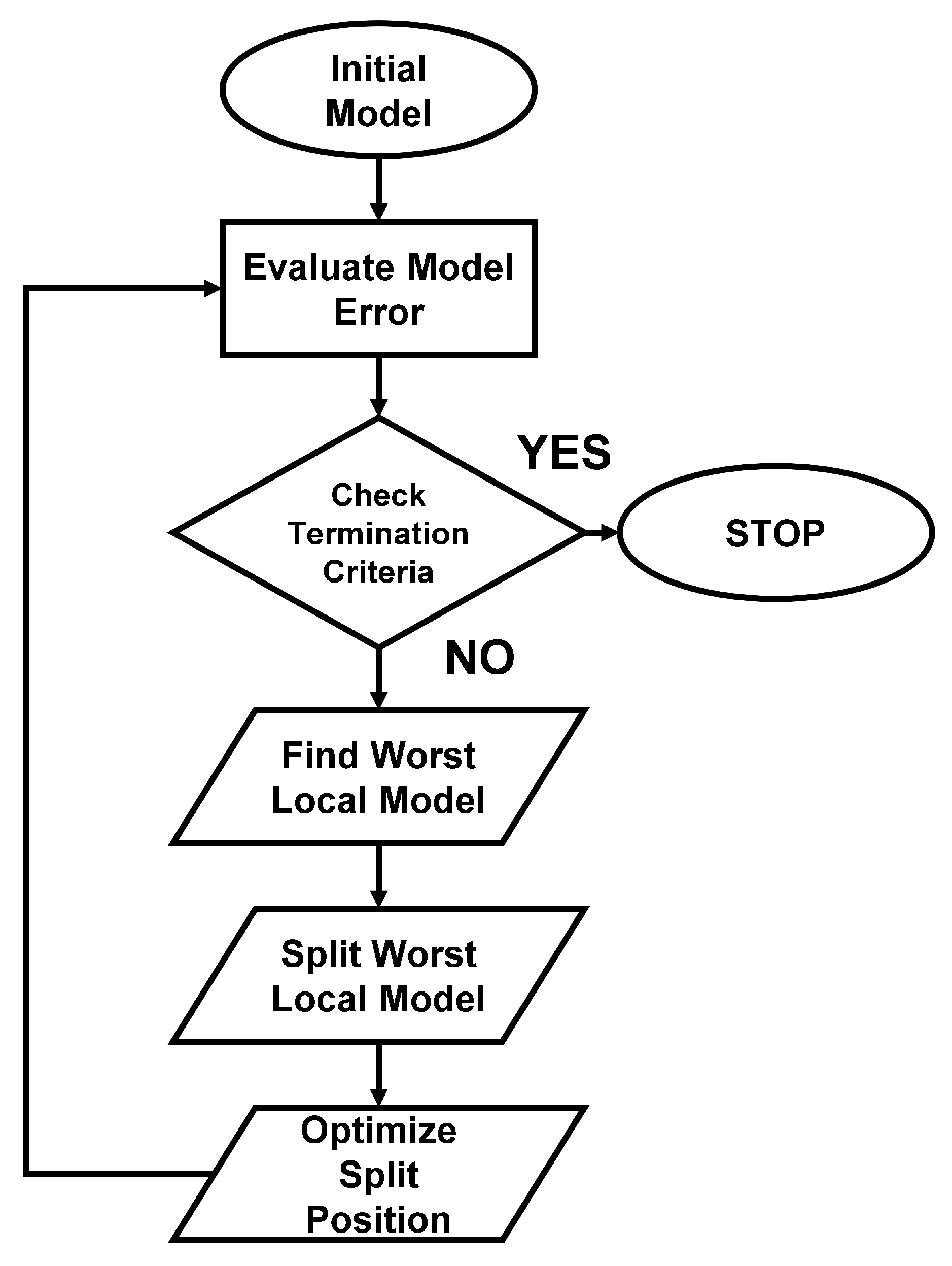
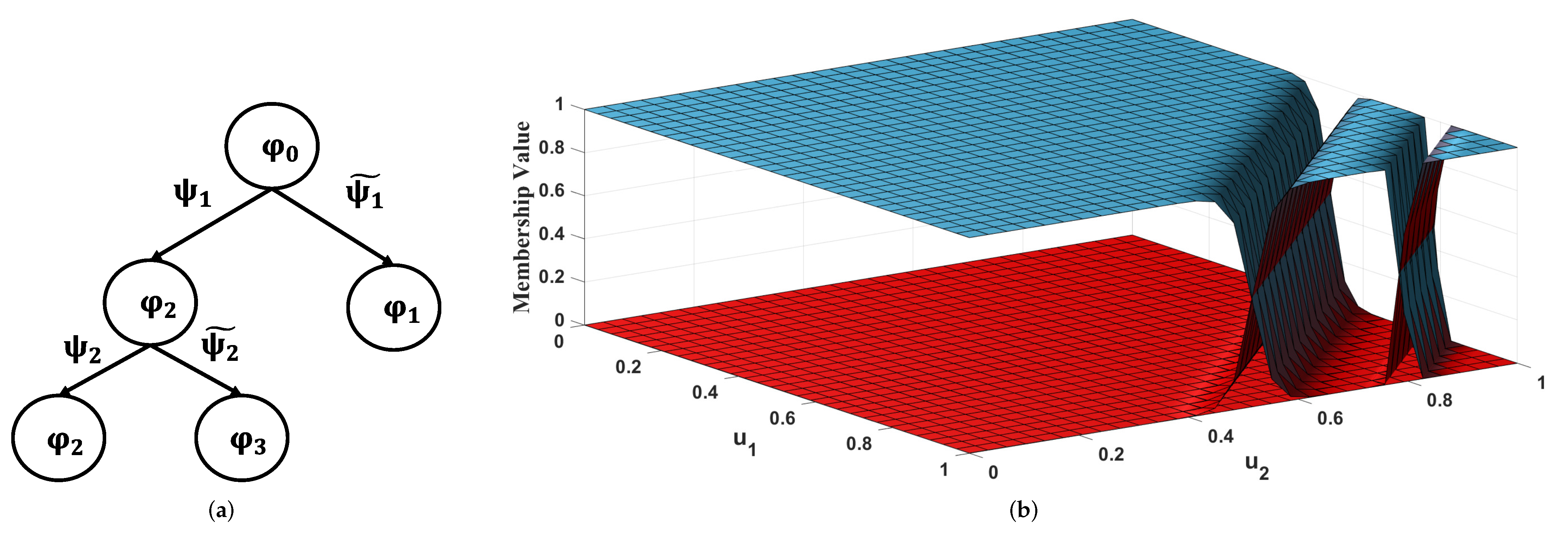
3. HILOMOT Algorithm

The HILOMOT algorithm is an iterative LMN training algorithm presented in [59]. Figure 2 depicts the algorithm flow chart for the HILOMOT algorithm. It is a heuristic tree construction method, which hierarchically divides the input space into sub-regions defined by the validity functions, ${\phi }_i$. Each sub-region holds a Local Linear Model (LLM), ${\widehat{y}}_i$, which portrays the local behavior of the process. Each LLM is defined by:

$${\widehat{y}}_i=\underline{x}·{\underline{w}}_i,$$

(1)

Here, ${\underline{w}}_i$ is the parameter vector for the ith local model and vector $\underline{x}$ spans the local model input space. The aggregation of the outputs of all the local models gives the overall output of the system. Since LMN is also a kind of neuro-fuzzy model, the validity functions are regarded as the rule premises and the LLMs are regarded as the rule consequents and separating the input spaces for the rule space and the consequent space allows the opportunity to include prior knowledge about the system behavior, such as strong nonlinearity, which is a significant feature of nonlinear systems identification [59].

The HILOMOT algorithm replaces the worst local model with new local models at every iteration. Figure 3 demonstrates the hierarchical decomposition of the input space.

For this purpose, the HILOMOT algorithm exploits the sigmoid function as the splitting function, unlike the LOLIMOT algorithm, which employs the orthogonal Gaussian functions. The benefit of using the sigmoid function is that it can be oriented in any direction with flexibility [86]. At every iteration, the input space of the worst local model is divided into two consequent sub-local models whose validity is defined by the new sigmoid, ${\psi }_i$, and its complementary sigmoid, $\tilde{\psi }$, respectively. Thus, at every iteration, the complexity of the model increases and thereby also improves the approximation of the model. A sigmoid function is defined by:

$${\psi }_i\left(\underline{z}\right)=\frac{1}{1+e^{(v_0+v_1{z}_1+\cdots +v_{nz}{z}_{nz})}},$$

(2)

Here, the $\underline{v}$ is the parameter vector, and $\underline{z}$ span the rule premise. The parameter vector influences the orientation of the split, and the split determines the accuracy of the model. Hence, finding the best local models involves estimating the optimal local model parameters, $\underline{w}$, and estimating the optimal sigmoid parameter, $\underline{v}$. The optimal local model parameters can be calculated analytically by using the least square method, whereas estimating the optimal sigmoid parameter vector requires an expensive nonlinear optimization algorithm. However, as the parameter vector $\underline{v}$ also influences the steepness of the sigmoid function, optimizing this parameter vector to optimize the split increases the steepness, which results in the undesired sharp transition between the models. Thus, to eradicate the effect of the parameter vector on the gradient of transition, a parameter, $\kappa$, is introduced which normalizes the parameter vector [59] and affects the sharpness of the transition. It is defined as:

$$\kappa =\frac{20}{\parallel v\parallel ·\parallel \Delta c\parallel ·\sigma },$$

(3)

in [65]. Here, $\parallel v\parallel$ is the norm of the vector v, $\parallel \Delta c\parallel$ is the distance between the centers of the sub-models, and $\sigma$ is a smoothness parameter. The inclusion of the magnitude of the parameter vector normalizes the parameter vector and thus no longer impacts the steepness of the sigmoids. Therefore, finally, the equation of the sigmoid function is:

$$\psi \left(\underline{z}\right)=\frac{1}{1+e^{\kappa (v_o+v_1{z}_1+\cdots +v_{nz}{z}_{nz})}}.$$

(4)

On the other hand, considering the complete parameter vector, v is redundant as only the direction vector, ${\underline{v}}^{*}=[v_1,v_2,\cdots ,v_{nz}]$, influences the direction of the split. The distinction between the direction vector and the parameter vector is $v_0$, where the ratio $v_0/\parallel {\underline{v}}^{*}\parallel$ determines the perpendicular distance between the split position and the origin. Furthermore, the entire parameter vector decreases the efficiency of the optimizer as the optimizer deals with an over-determined problem. Consequently, this causes the calculation to become lengthy and results in a less optimal solution [65]. Thus, to avoid this problem, one parameter of the parameter vector is kept constant during the optimization to increase the flexibility of the optimization. Since $v_0$ is an offset and not associated with the input vector, it is kept constant, thereby increasing the optimizer’s degrees of freedom by one degree, and thus increasing the efficiency of the algorithm. Since the optimization of the split orientation requires an expensive nonlinear optimization algorithm, the following section presents the split optimization algorithms in detail.

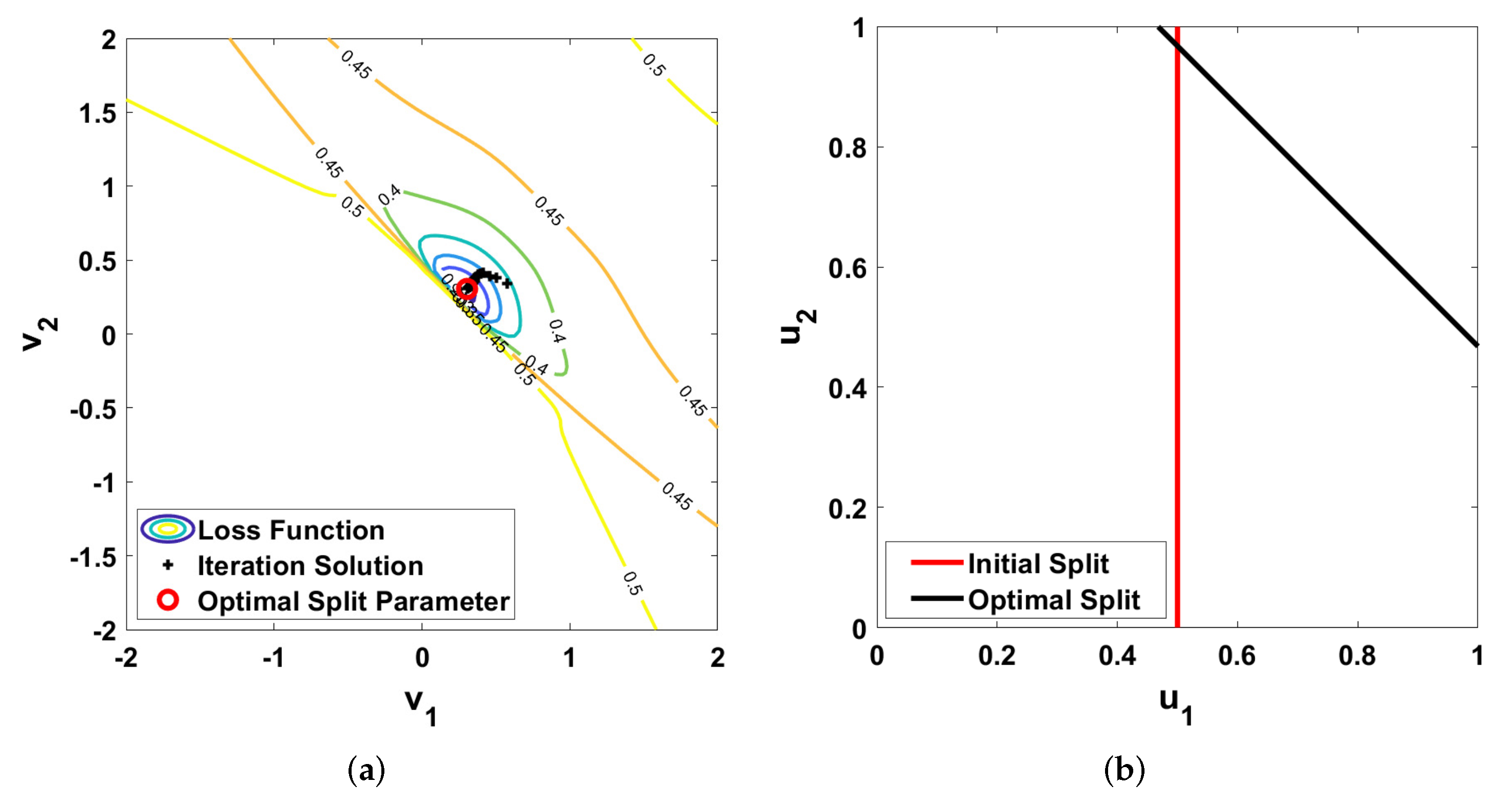
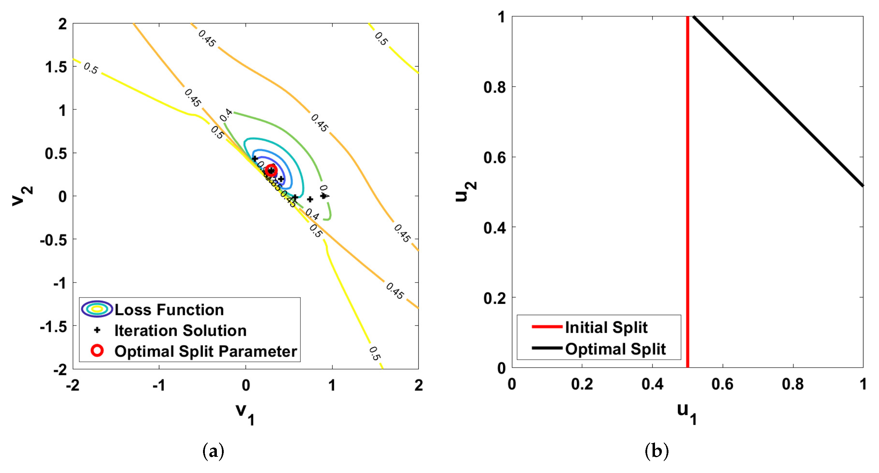
4. Split Optimization Algorithms

The HILOMOT algorithm requires optimization of the sigmoid parameter vector in every iteration to obtain the optimal split position of the validity functions. This presents a nonlinear optimization problem. Nonlinear optimization algorithms can be broadly classified as gradient-based and heuristic search-based algorithms. This paper presents the enhanced EM algorithm which is a gradient-based algorithm and enhanced PSO algorithm which is a heuristic search-based algorithm for the improvement of the HILOMOT training algorithm. A brief description of the optimization algorithms is presented below.

4.1. Expectation–Maximization (EM) Algorithm

The Expectation–Maximization (EM) algorithm is a method to heuristically improve the estimate of maximum likelihood parameters of a model with unobserved hidden variables. The optimal position or the validity of local models is unknown or hidden a priori during the training of LMN. Thus, the EM algorithm has been used to find the optimal split positions of the validity functions, and its convergence has been proven in [68,69]. The goal of the EM algorithm is to find the best model parameters in each iteration that would reduce the error of misclassification. The EM algorithm performs the Expectation (E)-step and then a Maximization (M)-step in each iteration. In the E-step, the local model parameters are calculated based on the current or initial estimate of the parameter vector, v, using the LS algorithm. Then, in the M-step, the reduced parameter vector, ${\underline{v}}^{*}$, is optimized to maximize the expectation of the model by reducing the misclassification error. The following steps formulate the iterative algorithm:

• Initialize $v_0$ and ${\underline{v}}^{*}$.
• Step 1: Calculate the validity functions.
• Step 2: Calculate the local model parameters $w_i$ of the local models.
• Step 3: Optimize the reduced parameter vector ${\underline{v}}^{*}$.
• Step 4: Repeat steps 1 to 4 until the stopping criteria are met.

4.2. Particle Swarm Optimization (PSO) Algorithm

PSO is one of the many nature-inspired meta-heuristic optimization algorithms, which was first used to study social behavior of different species in nature to fulfill their needs. However, further studies with PSO revealed its potential in solving different optimization problems. PSO is a global optimization algorithm which solves the issue of local optima of gradient descent algorithms at the cost of longer computational time. There are numerous variants of PSO, however, the basic variant of PSO initializes a swarm of particles (candidate solution) randomly, with a uniform distribution, over the entire search space. The particles are maneuvered around the input space using a simple mathematical formula. Each particle is assigned a velocity, which is determined by a few factors and affected by a few performance parameters that require heuristic tuning. The factors affecting the future velocity are its current velocity, a random component, the relevant particle’s best attained position, and the best attained position of the swarm. On the other hand, the parameters which greatly affect the performance of the algorithm are often termed as the exploration–exploitation trade off parameters. The exploration parameters help the particles to explore the complete search space in search of a global optimum, whereas the exploitation parameters try to narrow down a search around a promising candidate, to find the optimum precisely. The velocity equation is given by:

$$v_{i,j}^{k+1}=w\times v_{i,j}^k+c_1\times r_1\times (p_{i,j}^k-x_{i,j}^k)+c_2\times r_2\times (g_j^k-x_{i,j}^k)$$

(5)

Here, $v_{i,j}^k$ is the jth velocity component of the ith particle at the kth iteration, $x_{i,j}^k$ is the jth position component of the ith particle at the kth iteration, $p_{i,j}^k$ is the jth component of best position attained by the ith particle at the kth iteration, $g_j^k$ is the jth component of the best position attained in the swarm at the kth iteration, $c_1$ and $c_2$ acceleration parameters influence the experience of the particles, w is the inertial parameter, and $r_1$ and $r_2$ are the parameters adding randomness to the velocity. Finally, the position of the particles is updated using the following equation:

$$x_{i,j}^{k+1}=x_{i,j}^k+v_{i,j}^k,$$

(6)

PSO has been used to train an LMN in [70] due to its potential for finding the global optimum. PSO can be used to find the optimal local model parameters, $\underline{w_i}$, along with the reduced split position parameters, ${\underline{v}}^{*}$, however, this would unnecessarily increase the search space and consequently slow down the optimization process as the local model parameters can be estimated analytically. Hence, PSO is used only to find the optimal reduced split parameter vector and the LS algorithm is used to analytically estimate the local model parameters in each iteration. The termination criteria for the PSO algorithm are the maximum number of iterations or minimum change in error function. The complete PSO algorithm comprises the following steps:

• Select appropriate values for $w_{min}$, $w_{max}$, $c_1$, and $c_2$.
• Initialize position and velocities of the entire swarm.
• Evaluate the objective function and update p and g.
• Step 1: Calculate w.
• Step 2: Calculate velocity of each particle.
• Step 3: Update current position for each particle.
• Step 4: Evaluate the objective function with current position.
• Step 5: Update p and g if required.
• Step 6: Repeat steps 1 to 6 until the termination criteria are met.

4.3. Nested Optimization

Nested optimization, which was introduced in [59] and improved in [65], was used to train the HILOMOT algorithm. In this optimization algorithm, the loss function evaluation includes the evaluation of the local model parameters using the least square algorithm. A gradient descent algorithm is used to minimize the loss function, which is a function of the reduced parameter vector, ${\underline{v}}^{*}$. In every iteration, as the objective loss function is evaluated with the new reduced parameter vector, the new local model parameters are also calculated.

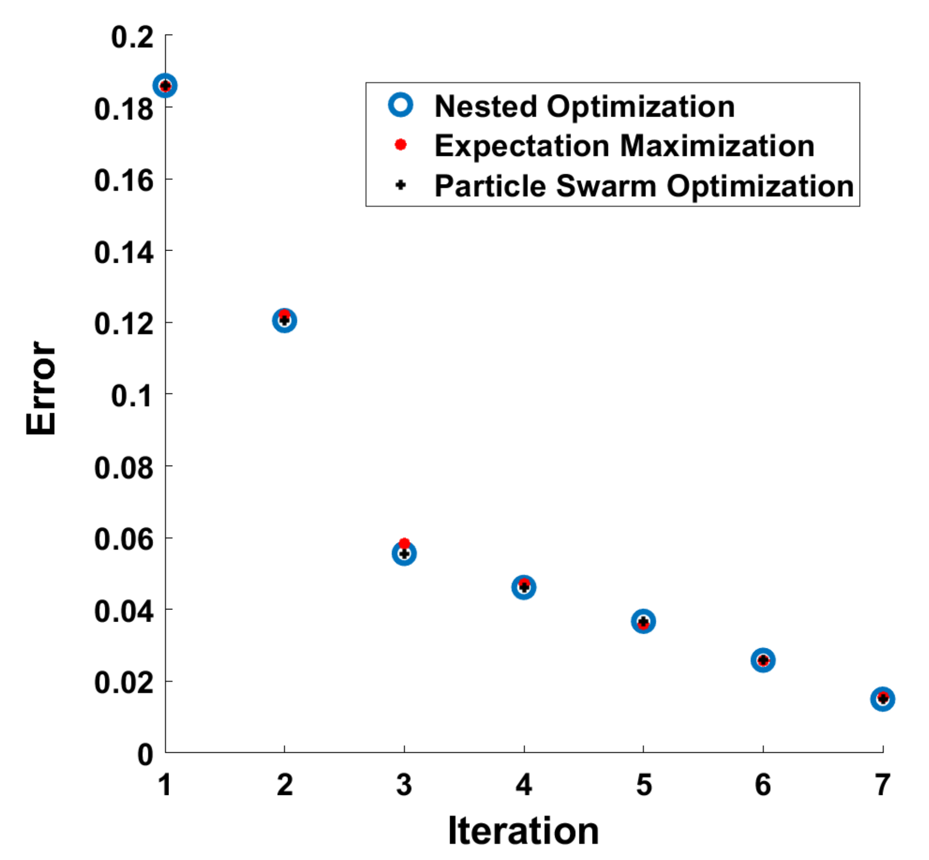
5. Results and Validation

The accuracy of the model approximation determines the performance of the HILOTMOT training algorithm, which further reflects the performance of the optimization algorithms. Hence, to analyze the performance of the optimization algorithms, several highly nonlinear functions with different structures and orders are fitted, and their results are compared. The “quality of solution” is chosen as the parameter to determine the performance of the optimization techniques in optimizing the HILOMOT training algorithm. Several aspects determine the quality of a solution, such as whether the solution reaches the optimum and whether the solution is a global or local optimum. Normalized Root Mean Squared Error (NRMSE), an excellent marker to determine the quality of solution, is chosen as the parameter for comparison in this paper. The equation to compute NRMSE is given by:

$$J\left({\underline{v}}^{*}\right)=\frac{\sqrt{{\displaystyle \sum _{i=1}^n}{e}_i^2\left({\underline{v}}^{*}\right)}}{\sqrt{{\displaystyle \sum _{i=1}^n}{(y_i-\overline{y})}^2}}$$

(7)

Table 1. Performance evaluation functions.

Symbol	Function	Reference
$f_1$	$y=\frac{u_1^3-1.5u_1^2+0.71u_1-5.105}{5}$	[46]
$f_2$	$y=\frac{u_1^4-1.9u_1^3+1.13u_1^2-.221u_1+5.0126}{5}$	[46]
$f_3$	$y=\frac{1}{0.1+\frac{(1-u_1)}{2}+\frac{(1-u_2)}{2}}$	[59,88,89]
$f_4$	$y=cos\left(4u_1\right)sin\left(4u_2\right)$	[46]
$f_5$	$y=\frac{(1-u_1^2)+100{(u_2-u_1^2)}^2}{100}$	[90]

lists the functions used in the evaluation process and

Table 2. Training error.

Function	NRMSE
Symbol	PSO	EM	NeO
$f_1$	0.017499	0.020576	0.018527
$f_2$	0.057793	0.061598	0.083211
$f_3$	0.011538	0.012598	0.013768
$f_4$	0.119732	0.112734	0.113158
$f_5$	0.054929	0.053244	0.055226

Underline and bold indicates the best solution and only bold indicates the second-best solution.

presents the results obtained from the evaluation process to compare and determine the superior optimization algorithm for enhancing the HILOMOT algorithm. The results were obtained using the MATLAB toolbox LMN-Tool [87].

From the results, it is conclusive that the accuracy of the approximated models achieved by different optimization algorithms is similar, with no significant differences. However, it is worth mentioning that for none of the function approximations did the Nested Optimization algorithm produce the best solution, and only for the functions $f_1$, $f_4$, and $f_6$ did the Nested Optimization algorithm produce the second-best solution. On the other hand, EM and Nested Optimization algorithms produced repeatable results, whereas the PSO-produced results were not repeatable due to its random initialization.

Table 3. Mean and standard deviation of the results from PSO algorithm.

Function	Mean	Standard Deviation (${10}^{-5}$)
$f_1$	0.017527	1.6636
$f_2$	0.057820	1.6927
$f_3$	0.011559	1.1638
$f_4$	0.119749	1.2787
$f_5$	0.054952	1.4889

presents the mean and standard deviation of ten optimization results of the PSO algorithm for each function. The standard deviations reveal that the results are concentrated near the mean and thus have a high confidence interval. The lowest optimization value for each function has been used for comparison in Table 2.

Furthermore, as HILOMOT iteratively increases the model’s accuracy, the model complexity increases at every iteration. Hence, the performance of the optimization algorithms is analyzed at different complexity levels. Moreover, as EM and nested algorithms are gradient descent algorithms and there was a difference in the model error, the optimization algorithms are further investigated for being susceptible to local optima. Therefore, the comparison of iterative optimization of the HILOMOT algorithm is presented with the help of an illustrative example. The function selected for demonstration is:

$$y=\frac{1}{0.1+\frac{(1-u_1)}{2}+\frac{(1-u_2)}{2}}$$

(8)

Figure 4 demonstrates the process described by Equation (8), which is highly nonlinear in a particular direction. According to Table 2, the PSO and EM algorithms produce the best and second-best results, respectively, in modeling this process. The reason behind this difference is further investigated and explained with the results demonstrated in Figure 5, Figure 6, Figure 7, Figure 8 and Figure 9.

Figure 5 demonstrates the complete partition plots for the individual optimization techniques. The partition plots show that PSO and EM algorithms placed more partitions in the direction of optimization than the Nested Optimization algorithm, consequently resulting in better approximation. Thus, the partition plots corroborate the findings of Table 2. Furthermore, Figure 6, Figure 7 and Figure 8 illustrate the loss function contour plots and partition plots after each iteration, and Figure 9 demonstrates the convergence of the HILOMOT algorithm with the three different optimization algorithms. The partition plots depict that the optimization algorithms found slightly different optimal splits despite having the same initiation in iteration 1. Hence, these slight differences accumulate over the iterations, resulting in the different partition plots and the overall approximation error. Moreover, the results in Figure 9 and the contour plots in each iteration demonstrate that the convergence rate in every iteration is similar with no significant differences, which further indicates that the algorithms were not prone to getting stuck in local optima. Therefore, finally, it can be concluded that the better approximation of EM and PSO algorithms resulted from their ability to place more partitions in the direction of nonlinearity than the Nested Optimization algorithms.

Finally, the HILOMOT algorithm is used to model the $N{O}_x$ emission process of a gas turbine power plant using the different optimization algorithms. $N{O}_x$ emission, a principal constituent of air pollution, is responsible for environmental problems such as acid rain, smog, ozone layer depletion, and ultimately global warming [91]. Hence, significant research is dedicated to building models for monitoring and controlling such emission processes. A novel data set from static measurement data has been introduced in [92] for Predictive Emission Monitoring System (PEMS) design. The paper discusses a handful of modeling approaches that are appropriate for designing predictive monitoring systems; however, these models do not provide significant insights for control engineers to design control systems that can optimize such processes. In order to compare the performance of the optimization algorithms, a model for the $N{O}_x$ emission as a function of the turbine inlet temperature and compressor discharge pressure from the static measurement data was trained using the HILOMOT algorithm with the three different optimization algorithms.

Table 4. Training error for gas turbine $N{O}_x$ emission model.

Normalized Root Mean Squared Error
PSO	EM	NeO
0.475962	0.479747	0.484005

Underline and bold indicates the best solution and only bold indicates the second-best solution.

presents the results of modeling a practical system for comparison between the performance of the algorithms.

The results demonstrates that PSO produced the best result and the Nested Optimization algorithm produced the worst result in modeling the real system.

However, even though the paper does not explicitly compare the methods for computational speed due to their different operation mechanisms, it is worth mentioning that the Nested Optimization algorithm was significantly faster than the other algorithms owing to its analytical gradient.

6. Conclusions

This paper presents the improved HILOMOT LMN training algorithm with enhanced EM and PSO optimization algorithms. The results are obtained by modeling several test functions and a practical system. The results demonstrate that the HILOMOT algorithm with the EM and PSO algorithms gave better solutions due to their ability to place more partitions in the direction of nonlinearity than the Nested Optimization algorithm. Consequently, despite being the faster algorithm, the Nested Optimization algorithm did not produce the best solution within the boundary of this work. Thus, the results indicate that the PSO and EM algorithms improved the HILOMOT algorithm.

References

1. Novak, A.; Simon, L.; Kadlec, F.; Lotton, P. Nonlinear system identification using exponential swept-sine signal. IEEE Trans. Instrum. Meas. 2009, 59, 2220–2229. [Google Scholar] [CrossRef] [Green Version]
2. Westwick, D.T.; Perreault, E.J. Closed-loop identification: Application to the estimation of limb impedance in a compliant environment. IEEE Trans. Biomed. Eng. 2010, 58, 521–530. [Google Scholar] [CrossRef] [PubMed] [Green Version]
3. Zhao, Y.; Westwick, D.T.; Kearney, R.E. Subspace methods for identification of human ankle joint stiffness. IEEE Trans. Biomed. Eng. 2010, 58, 3039–3048. [Google Scholar] [CrossRef] [PubMed]
4. Lai, C.Y.; Xiang, C.; Lee, T.H. Data-based identification and control of nonlinear systems via piecewise affine approximation. IEEE Trans. Neural Netw. 2011, 22, 2189–2200. [Google Scholar]
5. Talmon, R.; Kushnir, D.; Coifman, R.R.; Cohen, I.; Gannot, S. Parametrization of linear systems using diffusion kernels. IEEE Trans. Signal Process. 2011, 60, 1159–1173. [Google Scholar] [CrossRef] [Green Version]
6. Bloch, G.; Lauer, F. Reduced-size kernel models for nonlinear hybrid system identification. IEEE Trans. Neural Netw. 2011, 22, 2398–2405. [Google Scholar]
7. Chen, H.F. New approach to recursive identification for ARMAX systems. IEEE Trans. Autom. Control 2010, 55, 868–879. [Google Scholar] [CrossRef]
8. Chen, X.M.; Chen, H.F. Recursive identification for MIMO Hammerstein systems. IEEE Trans. Autom. Control 2010, 56, 895–902. [Google Scholar] [CrossRef]
9. Er-Wei, B. Non-Parametric Nonlinear System Identification: An Asymptotic Minimum Mean Squared Error Estimator. IEEE Trans. Autom. Control 2010, 55, 1615–1626. [Google Scholar] [CrossRef]
10. Han, M.; Fan, J.; Wang, J. A dynamic feedforward neural network based on Gaussian particle swarm optimization and its application for predictive control. IEEE Trans. Neural Netw. 2011, 22, 1457–1468. [Google Scholar] [CrossRef]
11. Kolodziej, J.R.; Mook, D.J. Model determination for nonlinear state-based system identification. Nonlinear Dyn. 2011, 63, 735–753. [Google Scholar] [CrossRef]
12. Jakubek, S.; Keuth, N. A local neuro-fuzzy network for high-dimensional models and optimization. Eng. Appl. Artif. Intell. 2006, 19, 705–717. [Google Scholar] [CrossRef]
13. Pottmann, M.; Pearson, R.K. Block-oriented NARMAX models with output multiplicities. AIChE J. 1998, 44, 131–140. [Google Scholar] [CrossRef]
14. Pearson, R.K.; Pottmann, M. Gray-box identification of block-oriented nonlinear models. J. Process Control 2000, 10, 301–315. [Google Scholar] [CrossRef]
15. Greblicki, W. Nonparametric identification of Wiener systems by orthogonal series. IEEE Trans. Autom. Control 1994, 39, 2077–2086. [Google Scholar] [CrossRef]
16. Eskinat, E.; Johnson, S.H.; Luyben, W.L. Use of Hammerstein models in identification of nonlinear systems. AIChE J. 1991, 37, 255–268. [Google Scholar] [CrossRef]
17. Hou, J.; Chen, F.; Li, P.; Zhu, Z. Gray-Box Parsimonious Subspace Identification of Hammerstein-Type Systems. IEEE Trans. Ind. Electron. 2021, 68, 9941–9951. [Google Scholar] [CrossRef]
18. Abba, S.; Abdulkadir, R.; Gaya, M.; Sammen, S.S.; Ghali, U.; Nawaila, M.; Oğuz, G.; Malik, A.; Al-Ansari, N. Effluents quality prediction by using nonlinear dynamic block-oriented models: A system identification approach. Desalin. Water Treat. 2021, 218, 52–62. [Google Scholar] [CrossRef]
19. Kashiwagi, H.; Rong, L. Identification of Volterra Kernels of Nonlinear Van do Vusse Reactor. Trans. Control Autom. Syst. Eng. 2002, 4, 109–113. [Google Scholar]
20. Chen, S.; Billings, S.A.; Luo, W. Orthogonal least squares methods and their application to non-linear system identification. Int. J. Control 1989, 50, 1873–1896. [Google Scholar] [CrossRef]
21. Piroddi, L.; Spinelli, W. An identification algorithm for polynomial NARX models based on simulation error minimization. Int. J. Control 2003, 76, 1767–1781. [Google Scholar] [CrossRef]
22. Di Nunno, F.; de Marinis, G.; Gargano, R.; Granata, F. Tide prediction in the Venice Lagoon using nonlinear autoregressive exogenous (NARX) neural network. Water 2021, 13, 1173. [Google Scholar] [CrossRef]
23. Di Nunno, F.; Granata, F.; Gargano, R.; de Marinis, G. Prediction of spring flows using nonlinear autoregressive exogenous (NARX) neural network models. Environ. Monit. Assess. 2021, 193, 1–17. [Google Scholar] [CrossRef] [PubMed]
24. Billings, S.A.; Wei, H.L. A new class of wavelet networks for nonlinear system identification. IEEE Trans. Neural Netw. 2005, 16, 862–874. [Google Scholar] [CrossRef] [Green Version]
25. Nash, D.A.; Ragsdale, D.J. Simulation of self-similarity in network utilization patterns as a precursor to automated testing of intrusion detection systems. IEEE Trans. Syst. Man Cybern. Part A Syst. Hum. 2001, 31, 327–331. [Google Scholar] [CrossRef]
26. Zhao, H.; Zhang, J. Nonlinear dynamic system identification using pipelined functional link artificial recurrent neural network. Neurocomputing 2009, 72, 3046–3054. [Google Scholar] [CrossRef]
27. Majhi, B.; Panda, G. Robust identification of nonlinear complex systems using low complexity ANN and particle swarm optimization technique. Expert Syst. Appl. 2011, 38, 321–333. [Google Scholar] [CrossRef]
28. De Veaux, R.D.; Psichogios, D.; Ungar, L. A comparison of two nonparametric estimation schemes: MARS and neural networks. Comput. Chem. Eng. 1993, 17, 819–837. [Google Scholar] [CrossRef]
29. Sahu, B.N.; Bisoi, R.; Samal, D. Identification of nonlinear dynamic system using machine learning techniques. Int. J. Power Energy Convers. 2021, 12, 23. [Google Scholar] [CrossRef]
30. Kumar, R.; Srivastava, S. A novel dynamic recurrent functional link neural network-based identification of nonlinear systems using Lyapunov stability analysis. Neural Comput. Appl. 2021, 33, 7875–7892. [Google Scholar] [CrossRef]
31. Gretton, A.; Doucet, A.; Herbrich, R.; Rayner, P.J.; Scholkopf, B. Support vector regression for black-box system identification. In Proceedings of the 11th IEEE Signal Processing Workshop on Statistical Signal Processing (Cat. No. 01TH8563), Singapore, 8 August 2001; pp. 341–344. [Google Scholar]
32. Dewapura, P.W.; Jayawardhana, K.; Harsha, A.M.; Abeykoon, S. Object Identification using Support Vector Regression for Haptic Object Reconstruction. In Proceedings of the 2021 3rd International Conference on Electrical Engineering (EECon), Colombo, Sri Lanka, 24 September 2021; pp. 144–150. [Google Scholar]
33. Salat, R.; Awtoniuk, M.; Korpysz, K. Black-box identification of a pilot-scale dryer model: A Support Vector Regression and an Imperialist Competitive Algorithm approach. IFAC-PapersOnLine 2017, 50, 1559–1564. [Google Scholar] [CrossRef]
34. Ažman, K.; Kocijan, J. Dynamical systems identification using Gaussian process models with incorporated local models. Eng. Appl. Artif. Intell. 2011, 24, 398–408. [Google Scholar] [CrossRef]
35. Yassin, I.M.; Taib, M.N.; Adnan, R. Recent advancements & methodologies in system identification: A review. Sci. Res. J. 2013, 1, 14–33. [Google Scholar]
36. Lee, Y.S.; Tsakirtzis, S.; Vakakis, A.F.; Bergman, L.A.; McFarland, D.M. A time-domain nonlinear system identification method based on multiscale dynamic partitions. Meccanica 2011, 46, 625–649. [Google Scholar] [CrossRef]
37. Babuška, R.; Verbruggen, H. Neuro-fuzzy methods for nonlinear system identification. Annu. Rev. Control 2003, 27, 73–85. [Google Scholar] [CrossRef]
38. Johansen, T.A.; Foss, B.A. Identification of non-linear system structure and parameters using regime decomposition. Automatica 1995, 31, 321–326. [Google Scholar] [CrossRef]
39. Johansen, T.A.; Foss, B.A. A NARMAX model representation for adaptive control based on local models. MIC J. 1992, 13, 25–39. [Google Scholar] [CrossRef]
40. Kumar, M.; Kumar, B.; Rani, A. Neuro-fuzzy based estimation of rotor flux for Electric Vehicle operating under partial loading. J. Intell. Fuzzy Syst. 2021, 41, 5653–5663. [Google Scholar] [CrossRef]
41. Wu, X.; Han, H.; Liu, Z.; Qiao, J. Data-Knowledge-Based Fuzzy Neural Network for Nonlinear System Identification. IEEE Trans. Fuzzy Syst. 2020, 28, 2209–2221. [Google Scholar] [CrossRef]
42. Johansen, T.A.; Foss, B.A. State-space modeling using operating regime decomposition and local models. IFAC Proc. Vol. 1993, 26, 39–42. [Google Scholar] [CrossRef]
43. Xu, J.; Huang, X.; Wang, S. Nonlinear model predictive control using adaptive hinging hyperplanes model. In Proceedings of the 48h IEEE Conference on Decision and Control (CDC) Held Jointly with 2009 28th Chinese Control Conference, Shanghai, China, 15–18 December 2009; pp. 2598–2603. [Google Scholar]
44. Nelles, O.; Sinsel, S.; Isermann, R. Local basis function networks for identification of a turbocharger. In Proceedings of the UKACC International Conference on Control, Control ’96, Exeter, UK, 2–5 September 1996. [Google Scholar]
45. Takagi, T.; Sugeno, M. Fuzzy identification of systems and its applications to modeling and control. IEEE Trans. Syst. Man Cybern. 1985, 1, 116–132. [Google Scholar] [CrossRef]
46. Nelles, O.; Fink, A.; Isermann, R. Local linear model trees (LOLIMOT) toolbox for nonlinear system identification. IFAC Proc. Vol. 2000, 33, 845–850. [Google Scholar] [CrossRef]
47. Billings, S.A. Models for Linear and Nonlinear Systems. In Nonlinear System Identification; John Wiley & Sons: Hoboken, NJ, USA, 2013; Chapter 2; pp. 17–59. [Google Scholar] [CrossRef]
48. Li, J.; Bo, C.; Zhang, J.; Du, J. Fault diagnosis and accommodation based on online multi-model for nonlinear process. In International Conference on Intelligent Computing; Springer: Berlin/Heidelberg, Germany, 2006; pp. 661–666. [Google Scholar]
49. Selmic, R.R.; Lewis, F.L. Multimodel neural networks identification and failure detection of nonlinear systems. In Proceedings of the 40th IEEE Conference on Decision and Control (Cat. No. 01CH37228), Orlando, FL, USA, 4–7 December 2001; Volume 4, pp. 3128–3133. [Google Scholar]
50. Toivonen, H.T.; Sandström, K.V.; Nyström, R.H. Internal model control of nonlinear systems described by velocity-based linearizations. J. Process Control 2003, 13, 215–224. [Google Scholar] [CrossRef]
51. Cai, G.B.; Duan, G.R.; Hu, C.H. A velocity-based LPV modeling and control framework for an airbreathing hypersonic vehicle. Int. J. Innov. Comput. Inf. Control 2011, 7, 2269–2281. [Google Scholar]
52. Hartmann, B.; Nelles, O.; Belič, A.; Zupančič-Božič, D. Local model networks for the optimization of a tablet production process. In International Conference on Artificial Intelligence and Computational Intelligence; Springer: Berlin/Heidelberg, Germany, 2009; pp. 241–250. [Google Scholar]
53. Zhou, C.; Huang, S.; Xiong, N.; Yang, S.H.; Li, H.; Qin, Y.; Li, X. Design and analysis of multimodel-based anomaly intrusion detection systems in industrial process automation. IEEE Trans. Syst. Man Cybern. Syst. 2015, 45, 1345–1360. [Google Scholar] [CrossRef]
54. Vasu, J.Z.; Deb, A.K.; Mukhopadhyay, S. MVEM-based fault diagnosis of automotive engines using Dempster—Shafer theory and multiple hypotheses testing. IEEE Trans. Syst. Man Cybern. Syst. 2015, 45, 977–989. [Google Scholar] [CrossRef]
55. Tirado, J.M.; Higuero, D.; Isaila, F.; Carretero, J. Multi-model prediction for enhancing content locality in elastic server infrastructures. In Proceedings of the 2011 18th International Conference on High Performance Computing, Bengaluru, India, 18–21 December 2011; pp. 1–9. [Google Scholar]
56. Yager, R.R.; Grichnik, A.J.; Yager, R.L. A soft computing approach to controlling emissions under imperfect sensors. IEEE Trans. Syst. Man Cybern. Syst. 2013, 44, 687–691. [Google Scholar] [CrossRef]
57. Adeniran, A.A.; El Ferik, S. Modeling and identification of nonlinear systems: A review of the multimodel approach—Part 1. IEEE Trans. Syst. Man Cybern. Syst. 2016, 47, 1149–1159. [Google Scholar] [CrossRef]
58. Ltaief, M.; Abderrahim, K.; Abdennour, R.B.; Ksouri, M. Contributions to the multimodel approach: Systematic determination of a models’ base and validities estimation. Int. J. Autom. Syst. Eng. 2008, 2, 213–220. [Google Scholar]
59. Nelles, O. Axes-oblique partitioning strategies for local model networks. In Proceedings of the 2006 IEEE Conference on Computer Aided Control System Design, 2006 IEEE International Conference on Control Applications, 2006 IEEE International Symposium on Intelligent Control, Munich, Germany, 4–6 October 2006; pp. 2378–2383. [Google Scholar]
60. Ernst, S. Hinging hyperplane trees for approximation and identification. In Proceedings of the 37th IEEE Conference on Decision and Control (Cat. No. 98CH36171), Tampa, FL, USA, 18 December 1998; Volume 2, pp. 1266–1271. [Google Scholar]
61. Tao, Q.; Xu, J.; Li, Z.; Xie, N.; Wang, S.; Li, X.; Suykens, J.A.K. Toward Deep Adaptive Hinging Hyperplanes. IEEE Trans. Neural Netw. Learn. Syst. 2021. [Google Scholar] [CrossRef]
62. Breiman, L. Hinging hyperplanes for regression, classification, and function approximation. IEEE Trans. Inf. Theory 1993, 39, 999–1013. [Google Scholar] [CrossRef] [Green Version]
63. Pucar, P.; Millnert, M. Smooth Hinging Hyperplanes—An Alternative to Neural Nets; Linköping University: Linköping, Sweden, 1995. [Google Scholar]
64. Pucar, P.; Sjoberg, J. On the hinge-finding algorithm for hingeing hyperplanes. IEEE Trans. Inf. Theory 1998, 44, 1310–1319. [Google Scholar] [CrossRef] [Green Version]
65. Fischer, T.; Hartmann, B.; Nelles, O. Increasing the performance of a training algorithm for local model networks. In Proceedings of the World Congress of Engineering and Computer Science (WCECS), San Francisco, CA, USA, 25–27 October 2012. [Google Scholar]
66. Kuroda, M. Fast Computation of the EM Algorithm for Mixture Models. In Computational Statistics and Applications; IntechOpen: London, UK, 2021. [Google Scholar]
67. Panić, B.; Klemenc, J.; Nagode, M. Improved Initialization of the EM Algorithm for Mixture Model Parameter Estimation. Mathematics 2020, 8, 373. [Google Scholar] [CrossRef] [Green Version]
68. Gath, I.; Geva, A.B. Unsupervised optimal fuzzy clustering. IEEE Trans. Pattern Anal. Mach. Intell. 1989, 11, 773–780. [Google Scholar] [CrossRef]
69. Hametner, C.; Jakubek, S. Neuro-fuzzy modelling using a logistic discriminant tree. In Proceedings of the 2007 American Control Conference, New York, NY, USA, 9–13 July 2007; pp. 864–869. [Google Scholar]
70. Hametner, C.; Jakubek, S. Comparison of EM algorithm and particle swarm optimisation for local model network training. In Proceedings of the 2010 IEEE Conference on Cybernetics and Intelligent Systems, Singapore, 28–30 June 2010; pp. 267–272. [Google Scholar]
71. Moody, J.; Darken, C.J. Fast learning in networks of locally-tuned processing units. Neural Comput. 1989, 1, 281–294. [Google Scholar] [CrossRef]
72. Stokbro, K.; Umberger, D.; Hertz, J.A. Exploiting neurons with localized receptive fields to learn chaos. Complex Syst. 1990, 4, 603–622. [Google Scholar]
73. Gustafson, D.E.; Kessel, W.C. Fuzzy clustering with a fuzzy covariance matrix. In Proceedings of the 1978 IEEE Conference on Decision and Control including the 17th Symposium on Adaptive Processes, San Diego, CA, USA, 10–12 January 1979; pp. 761–766. [Google Scholar]
74. Wang, L.X.; Mendel, J.M. Fuzzy basis functions, universal approximation, and orthogonal least-squares learning. IEEE Trans. Neural Netw. 1992, 3, 807–814. [Google Scholar] [CrossRef] [PubMed] [Green Version]
75. Hohensohn, J.; Mendel, J.M. Two-pass orthogonal least-squares algorithm to train and reduce fuzzy logic systems. In Proceedings of the 1994 IEEE 3rd International Fuzzy Systems Conference, Orlando, FL, USA, 26–29 June 1994; pp. 696–700. [Google Scholar]
76. Mastorocostas, P.; Theocharis, J.; Kiartzis, S.; Bakirtzis, A. A hybrid fuzzy modeling method for short-term load forecasting. Math. Comput. Simul. 2000, 51, 221–232. [Google Scholar] [CrossRef]
77. Murry-Smith, R. A Local Model Network Approach to Nonlinear Modeling. Ph.D. Thesis, University of Strathclyde, Strathclyde, UK, 1994. [Google Scholar]
78. Breiman, L.; Friedman, J.H.; Olshen, R.A.; Stone, C.J. Classification and Regression Trees; Routledge: New York, NY, USA, 2017. [Google Scholar]
79. Sugeno, M.; Kang, G. Structure identification of fuzzy model. Fuzzy Sets Syst. 1988, 28, 15–33. [Google Scholar] [CrossRef]
80. Nelles, O. Nonlinear System Identification; IOP Publishing: Bristol, UK, 2002. [Google Scholar]
81. Glass, L.; Hilali, W.; Nelles, O. Compressing Interpretable Representations of Piecewise Linear Neural Networks using Neuro-Fuzzy Models. In Proceedings of the 2021 IEEE Symposium Series on Computational Intelligence (SSCI), Orlando, FL, USA, 5–7 December 2021; pp. 1–8. [Google Scholar]
82. Zavřel, J.; Jílek, M.; Šika, Z.; Beneš, P. Dexterity Optimization for Tensegrity Structures Using Local Linear Model Trees. In Proceedings of the 2021 9th International Conference on Control, Mechatronics and Automation (ICCMA), Luxembourg, 11–14 November 2021; pp. 46–49. [Google Scholar]
83. Ramezani-Khansari, E.; Tabibi, M.; Moghadas Nejad, F. Estimating Lane Change Duration for Overtaking in Nonlane-Based Driving Behavior by Local Linear Model Trees (LOLIMOT). Math. Probl. Eng. 2021, 2021, 4388776. [Google Scholar] [CrossRef]
84. Tabatabaei, M.; Kimiaefar, R.; Hajian, A.; Akbari, A. Robust outlier detection in geo-spatial data based on LOLIMOT and KNN search. Earth Sci. Inform. 2021, 14, 1065–1072. [Google Scholar] [CrossRef]
85. Schüssler, M.; Münker, T.; Nelles, O. Local model networks for the identification of nonlinear state space models. In Proceedings of the 2019 IEEE 58th Conference on Decision and Control (CDC), Nice, France, 11–13 December 2019; pp. 6437–6442. [Google Scholar]
86. Hartmann, B.; Nelles, O. Advantages of hierarchical versus flat model structures for high-dimensional mappings. In Proceedings of the 19th Workshop on Computational Intelligence Publication Series of the Institute for Applied Computer Science / Automation Technology, Dortmund, Germany, 2–4 December 2009; Volume 19, pp. 87–100. [Google Scholar]
87. Hartmann, B.; Ebert, T.; Fischer, T.; Belz, J.; Kampmann, G.; Nelles, O. LMNTOOL—Toolbox zum automatischen Trainieren lokaler Modellnetze. In Proceedings of the 22th Workshop Computational Intelligence, Dortmund, Germany, 27–28 November 2014; pp. 341–355. [Google Scholar]
88. Hartmann, B.; Nelles, O.; Skrjanc, I.; Sodja, A. Supervised hierarchical clustering (SUHICLUST) for nonlinear system identification. In Proceedings of the 2009 IEEE Symposium on Computational Intelligence in Control and Automation, Nashville, TN, USA, 30 March–2 April 2009; pp. 41–48. [Google Scholar]
89. Bänfer, O.; Hartmann, B.; Nelles, O. Comparison of different subset selection algorithms for learning local model networks with higher degree polynomials. In Proceedings of the 2010 11th International Conference on Control Automation Robotics & Vision, Singapore, 7–10 December 2010; pp. 30–35. [Google Scholar]
90. Trelea, I.C. The particle swarm optimization algorithm: Convergence analysis and parameter selection. Inf. Process. Lett. 2003, 85, 317–325. [Google Scholar] [CrossRef]
91. Skalska, K.; Miller, J.S.; Ledakowicz, S. Trends in NOx abatement: A review. Sci. Total Environ. 2010, 408, 3976–3989. [Google Scholar] [CrossRef] [PubMed]
92. Kaya, H.; Tüfekci, P.; Uzun, E. Predicting co and no x emissions from gas turbines: Novel data and a benchmark pems. Turk. J. Electr. Eng. Comput. Sci. 2019, 27, 4783–4796. [Google Scholar] [CrossRef]
Figure 1. LMN structure with M neurons for n inputs [65].
Electronics 11 00729 g001
Figure 2. Algorithm flowchart for the HILOMOT algorithm.
Electronics 11 00729 g002
Figure 3. (a) The model tree and (b) the corresponding hierarchical decomposition.
Electronics 11 00729 g003
Figure 4. Function in Equation (8).
Electronics 11 00729 g004
Figure 5. Complete partition plots for the optimization techniques. (a) Complete partition with NA. (b) Complete partition with EM algorithm. (c) Complete partition with PSO.
Electronics 11 00729 g005aElectronics 11 00729 g005b
Figure 6. The loss function and model partition for EM algorithm after iteration 1. (a) Loss function. (b) Model partition.
Electronics 11 00729 g006
Figure 7. The loss function and model partition for NeO algorithm after iteration 1. (a) Loss function. (b) Model partition.
Electronics 11 00729 g007
Figure 8. The loss function and model partition for PSO algorithm after iteration 1. (a) Loss function. (b) Model partition.
Electronics 11 00729 g008
Figure 9. Convergence of the HILOMOT algorithm.
Electronics 11 00729 g009