Application of IoT Quadrotor Dynamics Simulation

Abstract

With the development of consumer-grade drone products, drones have been good carriers for many IoT (Internet of Things) applications, especially as a part of edge computing to deliver things, collect data, or monitor objects. This paper develops a Unity3D-based quadrotor dynamics simulation component on the original platform. In order to complete the simulation, a force analysis is performed for the quadrotor to establish a physical model based on Newtonian mechanics and Euler angles, and a PID (Proportion Integral Differential)-based control model is developed based on this physical model, which performs a fixed-point control for the simulation. The component introduces weather impact factors into the physical model through an environmental computational model and presents weather effects to the user interface. In addition, we add a scene customization function and a multi-aircraft formation flight function to the original simulation, and optimize the interface presentation scheme for multi-aircraft formation flight. The quadrotor simulation model in this paper solves the problem that the original simulation system is not realistic enough and significantly improves the usability and stability of quadrotors working in the IoT area.

1. Introduction

Breguet made the first quadrotor in 1907. For the first time, he proposed the solution that uses four rotors to provide power to offset a craft’s own moment of inertia. However, it was not widely applied because of its difficult control, complex mechanical structure, and large size. In the 1990s, miniaturized electronic sensors, micro controllers, miniaturized batteries, and many other technologies have improved quadrotors. Thus, multirotors, especially quadrotors, become a research hot spot [1]. In Japan, the small quadrotor, Kenyence Gyrosaucer, appeared in the market as a toy in the early 21st century [2].

In August 2013, the PX4 developer team and 3D Robotics developed the opensource autopilot hardware Pixhawk, which raised the reliability of the craft. In the past 10 years, UAV (Unmanned Aerial Vehicle, also known as drone) manufacturers, such as DJI, Parrot, and Yuneec, have released many mini quadrotor drones.

There is also a large demand for UAVs in the IoT (Internet of Things) area, such as in edge computing and fog computing area [3], communication area [4], and many other fields. Installing a UAV or collections of UAVs has become a reality for applications in many fields [5]. For instance, we can use UAVs to deliver goods [6], monitor storehouses, maintain public safety, etc.

UAVs are vulnerable to certain weather conditions when flying outdoors [7], ergo it is necessary to consider weather conditions when building a simulation model for UAVs.

We carried out the force analysis for the flying quadrotor. We established a physical model based on Newtonian mechanics and Euler angles. Thus, a PID-based control model is established according to the physical model. We perform fixed-point control on the quadrotor in a physical simulation to complete the entire simulation.

In this paper, the weather-influencing factors are introduced into the physical model through an environmental calculation model, and a method to estimate the environmental parameters based on the weather is provided, thus completely adding the weather-influencing factors.

2. Related Work

According to the power position, the structure of quadrotors is divided into two types: a cross shape and X-shape. The cross-shaped quadrotor is cross-symmetrical, and its four rotors are distributed in four directions: front, rear, left, and right. The X-shape quadrotor is X-shaped symmetrical, with the main part in the center of the X-shape, and the four rotors distributed on the four corners.

In the past 10 years, there have been many researches about the dynamic model of quadrotors. Some of these researches [8,9,10,11,12] use the Newton–Euler method, which calculates dynamics and motion equations based on Newton’s second law and Euler law, to create a simulation. Others [12,13,14] use the Euler–Lagrange method, which calculates a dynamics model using Lagrangian mechanics to express the quadrotor as a physical system with six degrees of freedom.

Research has been conducted in relation to the simulation of quadrotors under wind conditions. Khan proposed a dynamic model of the rotor moving in wind [15]. The model obtains the differential thrust model though MT (Momentum Theory) and BET (Blade Element Theory) to calculate induction speed in real time. Khan then differentiates the thrust of the blade airfoil section and integrates so as to obtain the total thrust.

Fernando [16] uses the Newton–Euler method to model quadrotor dynamics. Tran [17] and Massé [12] proposed a look-up table method for calculating the total force of the rotor and wind interaction based on Khan’s model. Refs. [8,14] used a method based on a PID controller. The work of [9] adopted an adaptive inverse control method. Ref. [11] used the ADRC (Active Disturbance Rejection Control) algorithm to build models.

3. Theoretical Basis of the Components

3.1. Representation of the Coordinate System

Our simulation model will be implemented with Unity. As Unity’s coordinate system design will be used, which has a left-handed coordinate system with the x-axis to the right, the y-axis up, and the z-axis forward.

This model will use Euler angles to define the attitudes of the quadrotor. The Euler angle is an intuitive rigid body attitude representation method. By decomposing the rigid body rotation into three basic rotations around a fixed axis, the rotation state is converted into a three-dimensional vector representation [8].

In flight control, the order of yaw-pitch-roll is usually used to decompose the overall rotation to define the Euler angle of the rotation. Therefore, defined by the above left-handed coordinate system, the Euler angles are defined as follows:

$$\mathrm{\Theta }={(\theta ,\psi ,\varphi )}^T$$

(1)

where $\theta$ refers to the pitch angle of the quadrotor (down direction from the quadrotor’s front perspective is positive), $\psi$ refers to the yaw angle (clockwise direction from above is positive), and $\varphi$ refers to the roll angle (down direction from the left-side perspective is positive).

Calculated by triangular transformation, the relation between the angular velocity $\omega ={\left({\omega }_x,{\omega }_y,{\omega }_z\right)}^T$ and Euler angle’s rate of change $\dot{\mathrm{\Theta }}$ is:

$$\left(\begin{array}{c}{\omega }_x\\ {\omega }_y\\ {\omega }_z\end{array}\right)=\left(\begin{array}{ccc}1& 0& -sin\theta \\ 0& cos\varphi & sin\varphi cos\theta \\ 0& -sin\varphi & cos\varphi cos\theta \end{array}\right)\left(\begin{array}{c}\dot{\theta }\\ \dot{\psi }\\ \dot{\varphi }\end{array}\right).$$

(2)

It can be calculated through triangular transformation, defined by the Euler angle, the vector ${\left(x^{\prime },y^{\prime },z^{\prime }\right)}^T$ in the body coordinate system can be converted to the vector ${\left(x,y,z\right)}^T$ in the geodetic coordinate system:

$$\left(\begin{array}{c}x\\ y\\ z\end{array}\right)=\left(\begin{array}{ccc}sin\varphi sin\psi sin\theta +cos\varphi cos\psi & -sin\varphi cos\psi +sin\psi sin\theta cos\varphi & sin\psi cos\theta \\ sin\varphi cos\theta & cos\varphi cos\theta & -sin\theta \\ sin\varphi sin\theta cos\psi -sin\psi cos\varphi & sin\varphi sin\psi +sin\theta cos\varphi cos\psi & cos\psi cos\theta \end{array}\right)\left(\begin{array}{c}{x}^{\prime }\\ y^{\prime }\\ z^{\prime }\end{array}\right).$$

(3)

3.2. Physical Model of the Quadrotor

3.2.1. Force Analysis of the Quadrotor

This paper will use the Newtonian mechanics method to build the dynamics model of the quadrotor.

At first, the force analysis of the quadrotor in the running state is shown in Figure 1.

Figure 1 shows the force generated by the four drone rotors of the quadrotor drone from the top view. It can be seen that the four rotors rotate in different directions, the adjacent rotors rotate in opposite directions, and the oblique rotors rotate in the same direction.

According to the aerodynamic model, when a single rotor turns, it provides an upward lift proportional to the square of the rotor’s angular velocity. With ${\omega }_i$ representing the angular velocity of the four rotors, and $T_i$ representing the lift of the four rotors, there are:

$$T_i=K_T·{\omega }_i^2.$$

(4)

The direction of lift appears to be upward along the quadrotor coordinate system.

According to Newton’s third law and aerodynamic model [8], when the rotor turns, it also produces a counter-torque to the drone in the opposite direction of rotation $Q_i$:

$$Q_i=K_Q·{\omega }_i^2.$$

(5)

The direction of the counter torque is opposite to the rotation direction of the corresponding rotor, that is, counterclockwise (downward) when i is an odd number, and clockwise (upward) when i is an even number.

In addition, due to the gyroscopic effect, a gyroscopic moment will also be generated when the attitude of the quadrotor changes:

$$M_{gyro}=J_M{\mathsf{\Omega }}_M\times {\omega }_i$$

(6)

where $J_M$ refers to moment of inertia of the motor shaft and propeller, ${\mathsf{\Omega }}_M$ refers to the angular velocity of the current rotation of the body, that is, the angular velocity of the procession of the gyro axis.

From Figure 2 we can know that the lift will provide a moment for the quadrotor:

$$L_i=R_i\times T_i$$

(7)

where $R_i$ refers to the displacement from the geometric center of the quadrotor to the rotation position of the rotor.

As shown in Figure 2, the quadrotor is also affected by gravity. Since the point of action of gravity can be equivalently regarded as the center of gravity, and there is a slight height difference between the center of gravity of the drone and the geometric center of gravity of the drone, the gravity will also generate a moment in which the quadrotor is tilted. From this, we can gain the gravity and gravitational moment of the object:

$$G=mg$$

(8)

$$M_G=d_i\times G$$

(9)

where m refers to the total weight of the quadrotor, g refers to the gravitational acceleration, and $d_i$ refers to the vector from the geometric center to the center of gravity of the quadrotor.

Based on the above mechanical model, the dynamics model of the quadrotor can be further calculated. Thus, the resultant force and moment of the quadrotor can be calculated. Then, the acceleration and angular acceleration of the quadrotor can be calculated.

3.2.2. Model of Wind Influence

The influence of air resistance is not discussed in the physical model in Section 3.2.1.

The resistance caused by air to the quadrotor is proportional to the speed of the air relative to the quadrotor [14].

The speed of the quadrotor relative to the air can be produced by subtracting the speed of the wind relative to the ground from the speed of the quadrotor relative to the ground.

Therefore, let $C_{drag}$ be the drag coefficient of the quadrotor; the air resistance can be:

$$D=C_{drag}·\left(v_{wind}-v\right)$$

(10)

where v refers to the velocity of the quadrotor, and $v_{wind}$ refers to the velocity of the wind.

Besides, the rotors are also affected by wind. Ref. [17] constructed a look-up table method according to the differential reasoning model of the additional force and moment that [15] exerts on the wind rotor. The method can be used to calculate the lateral thrust, extra lift, and extra moment of rotors with different speeds under different winds.

Table 1. APC 10 × 4.7SF rotor’s side thrust in the wind.

Side Thrust (N)	Wind Speed (m/s)	1	2	3	4	5
Rotating Speed (rpm)
2500		0.0107	0.0211	0.0318	0.0429	0.0541
3000		0.0131	0.0253	0.0380	0.0511	0.0645
3500		0.0154	0.0296	0.0443	0.0593	0.0748
4000		0.0178	0.0340	0.0506	0.0676	0.0850
4500		0.0201	0.0384	0.0570	0.0760	0.0953

shows the the side thrust table of the method.

3.2.3. Atmospheric Density Mechanics Model

In the equations above, coefficients $K_T$, $K_Q$, and $C_{drag}$ are all proportional to atmospheric density $\rho$.

Assume that the three coefficients are the values under standard atmospheric pressure, which meas ${\rho }_0$ = 1.293 kg/m${}^3$. Thus, when the atmospheric density is $\rho$, (4), (5), and (10) should be modified:

$$T_i=\frac{\rho }{{\rho }_0}{K}_T·{\omega }_i^2$$

(11)

$$Q_i=\frac{\rho }{{\rho }_0}{K}_Q·{\omega }_i^2$$

(12)

$$D=\frac{\rho }{{\rho }_0}{C}_{drag}·\left(v-v_{wind}\right).$$

(13)

3.2.4. Determination of Model Parameters

A large number of model coefficients are involved in the physical model. As for these coefficients, we used the presetting coefficients of the quadrotor “APC 10 × 4.7SF quadrotor-450 mm-1.5 kg-25 min-JFRC” provided by [18].

Some parameters are shown in

Table 2. Model parameters of the quadrotor.

Mark	Meaning	Value
m	Multicopter Mass	1.5 kg
g	Acceleration of Gravity	9.8 m/s${}^2$
j	Total Moment of Inertia	diag (1.318 × 10${}^{-2}$ kg·m${}^2$, 2.365 × 10${}^{-2}$ kg·m${}^2$, 1.318 × 10${}^{-2}$ kg·m${}^2)$
R	Distance of Motor to Center	0.225 m
$K_T$	Propeller Integrated Thrust Coef.	1.253 × 10${}^{-5}$ N/(rad/s)${}^2$
$K_Q$	Propeller Integrated Moment Coef.	1.852 × 10${}^{-7}$ N·m/(rad/s)${}^2$
$J_M$	Motor-Propeller Inertia	5.51 × 10${}^{-5}$ kg·m${}^2$
$C_{drag}$	Air-Drag Coef.	6.579 × 10${}^{-2}$ N/(m/s)
$v_{h,max}$	Max. Forward Speed	12.3 m/s
$n_{m}ax$	Max. Rotors Speed	6634.3 rpm

.

3.2.5. Conclusion of Dynamics Model

Decompose the above forces and moments into the world coordinate system. Merge (8), (11), and (13) separately in three dimensions and transform the force defined in the quadrotor coordinate system using (3), we can obtain the value of the combined force in three dimensions in the world coordinate system:

$$F_x=\frac{\rho }{{\rho }_0}{C}_{drag}\left(v_{wind,x}-v_x\right)+\frac{\rho }{{\rho }_0}{K}_T{\omega }^2\left(-sin\varphi cos\psi +sin\psi sin\theta cos\varphi \right)$$

(14)

$$F_y=\frac{\rho }{{\rho }_0}{C}_{drag}\left(v_{wind,y}-v_y\right)+\frac{\rho }{{\rho }_0}{K}_T{\omega }^{2}cos\varphi cos\theta -mg$$

(15)

$$F_z=\frac{\rho }{{\rho }_0}{C}_{drag}\left(v_{wind,z}-v_z\right)+\frac{\rho }{{\rho }_0}{K}_T{\omega }^2\left(sin\varphi sin\psi +sin\theta cos\varphi cos\psi \right).$$

(16)

3.3. Quadrotor Control Model

The control model established by this component for the quadrotor is generally based on the model provided by [18]. The principle of the control model will be explained below.

3.3.1. PID Controller

PID (Proportional Integral Derivative) controller consists of a proportional unit, integral unit, and derivative unit.

The input of the PID controller is the error value of the controlled quantity $e\left(t\right)$, and the output is $u\left(t\right)$. They are all functions of time t. A typical PID controller can be expressed by the following formula:

$$u\left(t\right)=K_{p}e\left(t\right)+K_i{\int }_0^{t}e\left(\tau \right)\mathrm{d}\tau +K_d\frac{\mathrm{d}}{\mathrm{d}t}e\left(t\right)$$

(17)

where $K_p$, $K_i$, and $K_d$, all non-negative, denote the coefficients for the proportional, integral, and derivative terms, respectively.

The proportional unit is the main part that responds to deviations in control. When there is a deviation, the proportional unit can change quickly to control the controlled quantity, so that the controlled quantity is corresponding.

The integral unit is to eliminate the accumulated error when the control reaches equilibrium. When there is a deviation, if there is a cumulative error in the value of the controlled quantity, only using the proportional coefficient will make the controlled quantity reach a balance within a certain fixed error. After adding the integral unit, the controlled quantity can reach the expected value.

The differential unit has the function of preventing overshoot.

Sometimes no integral unit or differential unit is needed, and the controller can complete the control on its own. A controller containing only a proportional unit is called a P controller, and similarly there are PI controls and PD controls.

For discrete time interval controllers, continuous integration of the integral unit and instant differentiation of the derivative unit are impossible. Therefore, this type of controller generally uses summation instead of integral and difference instead of differentiation:

$$u\left(t\right)=K_{p}e\left(t\right)+K_i\sum _{\tau =0}^{t}e\left(\tau \right)+K_d\left(e\left(t\right)-e\left(t-1\right)\right).$$

(18)

This formula can be simplified in the calculation. Subtract $u\left(t-1\right)$ from $u\left(t\right)$ to get:

$$u\left(t\right)-u\left(t-1\right)=K_p\left(e\left(t\right)-e\left(t-1\right)\right)+K_{i}e\left(t\right)+K_d\left(e\left(t\right)-2e\left(t-1\right)+e\left(t-2\right)\right).$$

(19)

Therefore, $u\left(t\right)$ becomes a value only related to $u\left(t-1\right)$, $e\left(t\right)$, $e\left(t-1\right)$, and $e\left(t-2\right)$. The content that needs to be stored while calculating is greatly simplified.

In the following, we use the letter P with different subscripts to refer to different PID controller functions that change over time, which can be written as $u\left(t\right)=P\left(e\left(t\right)\right)$.

3.3.2. Small-Angle Assumptions of the Model

A quadrotor can only fly normally when the tilt angle is very small. If the Euler angle is too large, the motion state of the quadrotor will be extremely unstable. If the quadrotor is turned upside down for a long time, it is no longer possible to control the rotor to climb upward because the lift’s direction is the same as the gravity’s. Thus, the quadrotor will inevitably enter a state of falling down with positive feedback. Therefore, in the following derivation of the control model, we believe that during the flight of the quadrotor, the pitch and roll angles are both small angels, which satisfies:

$$sin\varphi \approx \varphi ,cos\varphi \approx 1,sin\theta \approx \theta ,cos\varphi \approx 1.$$

(20)

Meanwhile, in the control of the quadrotor, this component should also try to avoid a situation in which the small angle assumption is destroyed or the quadrotor is out of control. This will be done by adding saturation to the control parameters.

3.3.3. Deductions from Physical Model

It can be seen from (14) and (16) that the acceleration of the quadrotor in the horizontal direction is composed of the acceleration of the air resistance and the acceleration of the lift provided by the propeller. It should be noted that if we take m and $C_{drag}$ from Table 2, and take the simulation time interval $t=0.02$ s, the change value of the air resistance item is always $-0.08\%$ of the force value calculated in the previous simulation time interval (before $0.02$ s).

For the PID control model, such a small change ratio value makes it possible to regard the air resistance part of a constant with disturbance, which is solved by the integral unit in the PID control. If the air resistance term is regarded as a constant, the acceleration value of the UAV is directly related to the trigonometric function value of the attitude angle when the total lift provided is certain. According to the small angle hypothesis in Section 3.3.2, the trigonometric function value of the attitude angle can be understood as $\varphi$, $\theta$ itself, that is to say, the acceleration value of the drone in the horizontal direction can be compared with the attitude The angle value itself is directly related. Due to the proportional characteristics of PID, the attitude angle can be directly equivalent to the horizontal force to add to the control. With this, the control of the quadrotor can be decomposed into two parts: position control and attitude control.

3.3.4. Control Goal

Firstly, before processing the control model, we need to determine the control goal of this component. Therefore, we must proceed from the requirements and observe what kind of instructions the component needs to support. The instructions that this component needs to support are shown in

Table 3. Instructions of the quadrotor.

Instruction	Meaning	Return Value
takeoff	Let the quadrotor take off	ok/error
land	Let the quadrotor land	ok/error
emergency	Stop the motor immediately	ok/error
up x	fly upward x cm (x = 20∼500)	ok/error
down x	fly downward x cm (x = 20∼500)	ok/error
forward x	fly forward x cm (x = 20∼500)	ok/error
back x	fly backward x cm (x = 20∼500)	ok/error
cw x	Rotate clockwise x° (x = 1∼360)	ok/error
ccw x	Rotate anticlockwise x° (x = 1∼360)	ok/error
go x y z	Fly to coordinate (x, y, z) (x, y, z = 20∼500)	ok/error
speed x	Set the current speed to x m/s x = 0.1–10	ok/error

.

It can be seen that our goal is to move the quadrotor to a certain point, or to make the yaw attitude of the quadrotor reach a certain fixed value. If we let the quadrotor’s location be $\left(x,y,z\right)$, yaw attitude be $\psi$, target location be $\left(x_d,y_d,z_d\right)$, and target yaw attitude be ${\psi }_d$, our control goal can be written as:

$$t\to \infty ,\left(x,y,z\right)-(x_d,y_d,z_d)=\left(0,0,0\right),\psi -{\psi }_d=0.$$

(21)

3.3.5. Position Controller

The position controller aims at completing the first half of the Formula (21) so that the quadrotor can finally reach the target position. For this reason, this component divides the position control into two parts, the horizontal position channel and the vertical position channel according to the horizontal and vertical movement characteristics of the quadrotor.

On the horizontal position channel, as described by Section 3.3.3, the attitude angle can be directly equivalent to the horizontal force as the input of the position part. For the stability of the system, we adopt a PID controller composed of a two-stage PID. The expected speed is obtained from the position deviation via the outer loop PID, and then the expected force is obtained from the speed deviation via the inner loop PID, which is converted into the expected Euler angle:

$$\left(v_{xd},v_{zd}\right)=P_{hv}\left(\left(x,z\right)-\left(x_d,z_d\right)\right)$$

(22)

$$\left(-{\varphi }_d,{\theta }_d\right)\left(\begin{array}{cc}cos\psi & sin\psi \\ -sin\psi & cos\psi \end{array}\right)=P_{hf}\left(\left(v_x,v_z\right)-\left(v_{xd},v_{zd}\right)\right)$$

(23)

where $(x,z)$ refers to the quadrotor’s true horizontal position, $\left(x_d,z_d\right)$ refers to the expected horizontal position, $\left(v_{xd},v_{zd}\right)$ refers to the expected horizontal velocity, $\left(v_x,v_z\right)$ refers to the true horizontal velocity, ${\varphi }_d$ refers to the expected roll angle, and ${\theta }_d$ refers to the expected pitch angle. When ${\varphi }_d$ is positive, there will be an acceleration in the $-z$ direction ($\psi =0$), therefore we need to add a minus sign before ${\varphi }_d$.

The vertical position channel also adopts the cascade PID controller:

$$v_{yd}=P_{vv}\left(y-y_d\right)$$

(24)

$$f_t-G=P_{vf}\left(v_y-v_{yd}\right)$$

(25)

where $f_t$ refers to the expected lift and G refers to the impact of gravity.

When the fixed point is far away, the calculation result will make the two angle values of ${\theta }_d$ and $-{\varphi }_d$ too large, which will destroy the assumption of the small angle and the quadrotor will become abnormal. Therefore, in the horizontal position channel, it is necessary to saturate the velocity value that appears, that is, when the expected horizontal velocity $\left(v_{xd},v_{zd}\right)$ (the module length) exceeds the predetermined velocity (the value specified by the speed command) or the quadrotor maximum forward speed ($v_{h,max}$ in Table 2), we should limit the speed.

Similarly, the value of $\left({\theta }_d,-{\varphi }_d\right)$ also needs to be saturated, so that the size of the two angles does not exceed 30° (at this time, ${30}^{°}=0.5236$ rad, $\sin {30}^{°}=0.5$, the small angle assumption is still basically valid). In order to prevent the throttle speed from approaching the maximum throttle speed or being too small, making the speed too large or too small, and losing control space for the attitude control of the quadrotor (see Section 3.3.7 below for the reason), the vertical position channel also needs to be similarly saturated.

3.3.6. Altitude Controller

The attitude change is similar to the position situation, that is, the quadrotor’s torque in three directions can control its angular velocity, and the angular velocity further affects the attitude. In the physical model, the change in yaw angle is mainly produced by the changes in the anti-torque produced by the rotors rotating in different directions, while the pitch and roll angles are mainly produced by the lift moments produced by the different side rotors. The conversion paths of the two are quite different. Therefore, we divide the attitude controller into a pitch-roll channel and a yaw channel for processing.

For the pitch-roll channel, a similar cascade PID controller can be used:

$$\left({\omega }_{xd},{\omega }_{zd}\right)=P_{h\omega }\left(\left(\theta ,\varphi \right)-\left({\theta }_d,{\varphi }_d\right)\right)$$

(26)

$$\left({\tau }_{xd},{\tau }_{zd}\right)=P_{h\tau }\left(\left({\omega }_x,{\omega }_z\right)-\left({\omega }_{xd},{\omega }_{zd}\right)\right)$$

(27)

where ${\tau }_{xd}$ and ${\tau }_{zd}$ refer to the expected moment on the two axes. In order to maintain the control space for the quadrotor attitude, these two quantities also need to be saturated.

For the yaw channel, observe the cw and ccw commands. When the required rotation angle exceeds 180 degrees, if we control it directly, the controller will tend to make the drone rotate from the other side with a smaller rotation angle. Therefore, we need to saturate $\psi -{\psi }_d$ so that its absolute value does not exceed 90 degrees, and enter the radian value of the saturated angle $\Delta {\psi }_{sat}$ into the controller:

$$\Delta {\psi }_{sat}=max(min(\psi -{\psi }_d,90),-90)$$

(28)

$${\omega }_{yd}=P_{v\omega }\left(\Delta {\psi }_{sat}\right),{\tau }_y=P_{v\tau }\left({\omega }_y-{\omega }_{yd}\right).$$

(29)

3.3.7. Control Distributor

In Section 3.3.5 and Section 3.3.6, we present the calculation scheme of the controller to calculate the four control variables of expected lift $f_t$, pitching moment ${\tau }_x$, rolling moment ${\tau }_{zr}$, and yaw moment ${\tau }_y$.

Next, we need to assign the four mechanical parameters to the four rotors of the quadrotor.

Fortunately, the four control variables are the results of the PID controller. If the three coefficients of $K_p$, $K_i$, and $K_d$ are multiplied by a coefficient value, and then the output result of the PID controller is divided by this control value, the final result is exactly the same. In other words, the proportional coefficient of the PID controller itself can be used to eliminate the difference in coefficients in the control distributor.

Therefore, if the proportional coefficients between the square of the rotor speed and the mechanical quantities are integrated into the three control coefficients of the controller, the four control quantities passed into the control distributor can be regarded as relative values $f_{tr}$, ${\tau }_{xr}$, ${\tau }_{yr}$, and ${\tau }_{zr}$.

In this way, the influence coefficient of the same rotor on different control variables can be ignored.

Furthermore, our control model only needs to ensure that the relative proportions of different rotors to the same control quantity remain unchanged. By analyzing the contribution of each rotor to the various control variables, we get the control distribution model from the speed to the control variable:

$${\omega }_1^2=f_{tr}-{\tau }_{xr}+{\tau }_{zr}-{\tau }_{yr}$$

(30)

$${\omega }_2^2=f_{tr}+{\tau }_{xr}+{\tau }_{zr}+{\tau }_{yr}$$

(31)

$${\omega }_3^2=f_{tr}+{\tau }_{xr}-{\tau }_{zr}-{\tau }_{yr}$$

(32)

$${\omega }_4^2=f_{tr}-{\tau }_{xr}-{\tau }_{zr}+{\tau }_{yr}.$$

(33)

In an actual quadrotor, each rotor is driven by an electric motor. The power of the motor and the speed under load naturally have an upper limit. Therefore, in this paper, the rotor speed is saturated between 0 and the maximum speed (that is, ${\omega }_{max}$ in Table 2). If we allow a certain control quantity to expand or contract, it will cause all the control values to be stuck at the maximum value or drop below 0, causing the control of other control quantities to be unsuccessful. Therefore, in the previous article, the four control variables are also saturated before input.

3.3.8. Determination of PID Parameters

After completing the design of the PID control model, it is necessary to determine the control coefficients in the PID model. We use Python to build a physical model and a control model [19], so as to more conveniently observe the quality of PID parameters.

The PID control parameters obtained in this paper are shown in

Table 4. PID control parameters.

Controller	$K_P$	$K_I$	$K_D$
$P_{hv}$	0.28	0	0
$P_{hf}$	3.7	0.04	0.003
$P_{vv}$	1.4	0	0
$P_{vf}$	80	1	0.3
$P_{h\omega }$	1.6	0	0
$P_{h\tau }$	0.7	0.02	0.01
$P_{v\omega }$	1.4	0	0
$P_{v\tau }$	12	2	0.1

.

3.4. Environmental Model

According to the previous model, the environmental factors that mainly affect UAV flight include wind and atmospheric density.

However, compared to other environmental conditions such as weather, temperature, and air pressure, atmospheric density itself is not a very intuitive physical attribute.

In order to improve the usability of the system, so that users can easily add weather influence factors, we present an environmental model, which can be used to estimate the atmospheric density through other environmental information.

The final formula for deriving atmospheric density is based on the Ideal Gas Law:

$$pV=nRT$$

(34)

where p refers to the pressure, V refers to the volume, n is the amount of substance of gas, R is the ideal gas constant, and T is the absolute temperature.

Considering that when M is taken as the average relative molecular mass of the gas, $\rho$ is the density of air, and m is the total mass of the gas, there are:

$$\rho V=m=nM.$$

(35)

The calculation formula of atmospheric density $\rho$ can be deduced:

$$\rho =\frac{p}{T}·\frac{M}{R}$$

(36)

where M is the average relative molecular mass of air, and its value is in a relatively stable state, so $\frac{M}{R}$ can be regarded as a constant $R_{specific}$. Through the ideal environment parameters (

Table 5. Ideal environment parameters.

Parameter	Value
Temperature T	25${}^{°}$/298.15 K
Atmospheric Pressure p	101.325 kPa
Atmospheric Density	1.1839 kg/m${}^3$

), the value of $R_{specific}$ can be calculated to complete the calculation of atmospheric density.

4. Component Implementation Scheme

4.1. Architecture Design

4.1.1. Simulation Technology

The quadrotor simulation component is embedded in a web page as a WebGL page element.

WebGL (short for Web Graphics Library) is a JavaScript API for rendering interactive 2D and 3D graphics within any compatible web browser without the use of plug-ins. WebGL elements can be mixed with other HTML elements and composited with other parts of the page or page background [20].

Unity is a cross-platform game engine developed by Unity Technologies for the development of 3D games. The engine already supports almost all desktop, mobile, smart TV, game console, and virtual reality platforms, and supports packaging as WebGL components. The engine is also gradually expanding from games to other fields, and has been widely used in the film industry, transportation industry, architecture, engineering construction industry, and education industry [21].

We mainly use Unity to build the model, and finally package it as a WebGL component, which is integrated with other parts of the system to run on the web.

4.1.2. MVC-Like Architecture

The main structure of this component is similar to the MVC software architecture. MVC (Model View Controller) is a widely used software architecture model. Typical MVC software architecture is shown in Figure 3.

The software system using this architecture consists of the following three basic components:

• Model: In a general software system, the model part includes algorithms for designing business logic and database management for storing business data, which is the core logic component of the system. In our component, the model part is equivalent to a weather model, control model, physical model, and continuously updated runtime information.
• View: In ordinary software, the view part is the graphical interface part of the system, which contains all the data information displayed to the user. For our component, the view port is equivalent to the simulation interface rendered by Unity3D and the text content on the user interface.
• Controller: For general systems, the controller component is responsible for forwarding requests and processing the requests; for this component, the controller includes the part that sends and receives instructions from the main system and the part of the web page outside the component where the user enters the instruction information on the web page.

4.2. Specific Modules

The quadrotor simulation section contains the following submodules:

• Internal interactive module: Similar to controller components, it is responsible for processing internal interaction of other parts of the system, including initializing using configuration file, reading instructions, and returning when completing instructions.
• Motion computing module: Is part of the model component, including the physical model and control model. It receives instructions, and calculates the control and physical movement of the quadrotor. Thereby, it completes the simulation of the quadrotor.
• Environment module: Is also a part of the model component. It is responsible for saving and updating the environment status and sending weather condition information to the raining, snowing, and fogging system, which visualizes the weather condition.
• Camera control module: The module belongs to the view component, which is responsible for finding the best camera position, and performs the simulation display.

In addition, the view component also includes a function module with scene rendering and special effects display. These tasks are completed by the Unity engine.

4.3. Data Processing Flow

The data flow diagram in Figure 4 describes the general structure and data flow of our simulation component. It can be seen from Figure 4 that the initial configuration information and each instruction data are processed from the bottom-end web page terminals when running this simulation component. The initial configuration file is read through the internal interactive module, and then forwards to the motion status storage, physical model and control model part, and environment model part, to complete the initial scene arrangement.

During the simulation process, when a quadrotor flight instruction is read, it is processed by the instruction interactive module first, and is sent to the physical model and control model. The physical model and control model will update the quadrotor’s motion state based on the instruction information and environment condition. Then the motion state will be sent to view the display module and rendered by the Unity engine.

4.4. Internal Interactive Module

This module include two parts of work: environmental settings for simulated scenes and distribution of control instructions during the initial phase.

When the model is started and during the simulation, the web page can use the Unity’s own information transmitting scheme to trigger internal functions to send data to it, and call some internal methods.

We design a configuration file for initializing the environment in this module. The configuration file contains four parts: The metadata of the configuration file itself, necessary environment information that simulation needs, the initial scene information of the simulation, and the basic weather information. The configuration file is transferred into the model in the form of JSON.

In the initialization phase, the quadrotor object and obstacle objects will be placed in the scene. The environment information is then stored to the environment class. The weather information is sent to the special effect processing class.

During the flight, the module receives quadrotor flying instructions. After truncation of each individual instruction and judging correctness of the instruction, the module will forward the instruction to the instruction queue in the control model. If the instruction is incorrect, the module will report an error.

4.5. Motion Module

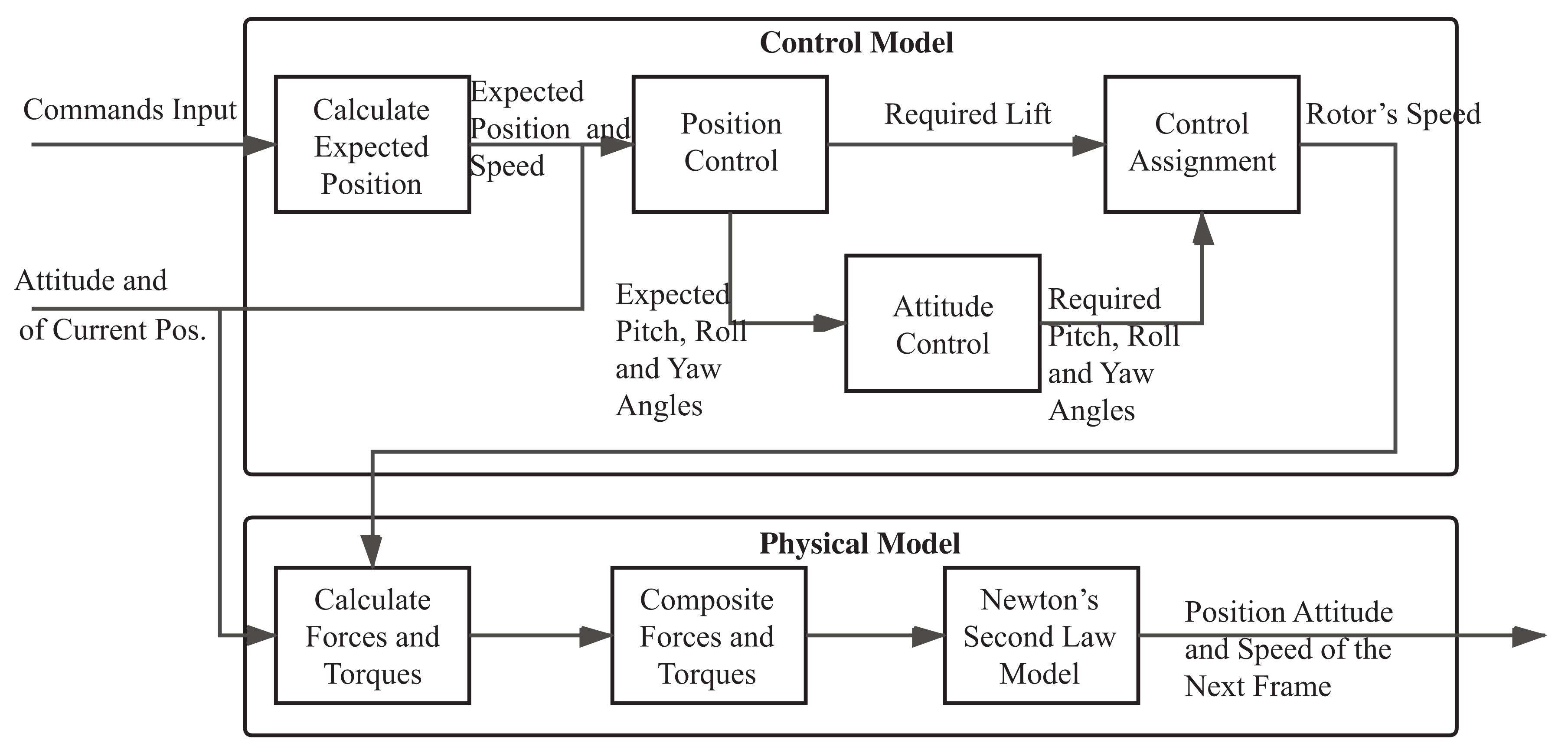
This module implements the physical model and control model described above. The computing process is as shown in Figure 5.

4.5.1. Implements of the Control Model

As Figure 5 shows, the calculation of the controller contains four steps:

• Calculate the target position as the expected position according to the content of the command.
• Control the location of the quadrotor: Based on the expected position, the current position, the expected speed, and the current speed, the casual PID controller with a two-layer PID controller is used to establish the position control model of the quadrotor. Then the three-dimensional acceleration vector is calculated, as required of the quadrotor.
• Control attitude of the quadrotor: The acceleration component, which is calculated by the position controller, of the two directions will be placed into a pitch and a roll expected attitude. Combined with the expected yaw attitude of the input, we use another casual PID controller with a two-layer PID controller to establish the model of the attitude control. Finally we calculate the angular acceleration on the three attitude required for the quadrotor.
• The angular acceleration value of the lift acceleration, pitch, yaw, and rolling are allocated to the four rotors. Finally, the rotor speed can be obtained.

4.5.2. Implements of the Physical Model

As shown in Figure 5, the calculation steps of the physical model are as follows:

• Calculate the force and torque of the quadrotor according to the formulas mentioned before.
• Composite the forces and torques.
• Obtain acceleration and angular acceleration using forces, torques, mass, and inertia torque. Then, the speed and angular velocity, position, and rotation is calculated.

When calculating the next frame, the result of the physical model will be sent to the control model. Then the model will continue calculating.

4.6. Camera Control Module

Design of Steps of Camera Controlling

Since we also support a multi-quadrotor flight, how to ensure that each quadrotor is in the lens display is a problem. The control scheme of the camera designed for this situation will be explained below. Control of the camera is divided into four steps:

• First, from the position of each quadrotor, set a distance range (10 m), which will be the range that must be displayed, such as Figure 6 shows.
• Then, the camera is forwarded to the right front 15 degree. Convert the coordinates to the camera parallel coordinate system and calculate the maximum value of the four directions, that must-display the range in the parallel coordinate system of the camera. Then use the cuboid range as the new must-display range, as shown in Figure 7.
• Calculate the minimum distance with the new range included, and the target position of the camera is derived, such as in Figure 8.
• Finally, move the camera smoothly by interpolation, using the components provided by Cinecamera.

4.7. Environment Module

4.7.1. Design of the Environment Module

We allow users to omit when providing parameters, and we provide a processing scheme that estimates atmospheric density values based on weather conditions and other physical quantities. When all environment information values are omitted, the workflow of the environment model is shown in Figure 9.

4.7.2. Result of the Environment Module

Using our physical model, control model, and environment model, it is possible to simulate the quadrotor flying in different weather conditions.

Figure 10 compares the movement of a quadrotor affected by the west wind and another not affected by wind.

Figure 11 shows that if the north wind appears suddenly, and the nature of the quadrotor’s movement.

Figure 12 compares that the movement of quadrotors between the quadrotors fly in normal air (the left one) and low-density air.

5. Test and Validation of the Simulation Model

According to the physical model and control model proposed above, we test and validate the simulation model without a weather condition and under various weather conditions.

Model Control Effect without Weather Condition

When the quadrotor is executing the command ”up 20”, the height change is shown in Figure 13.

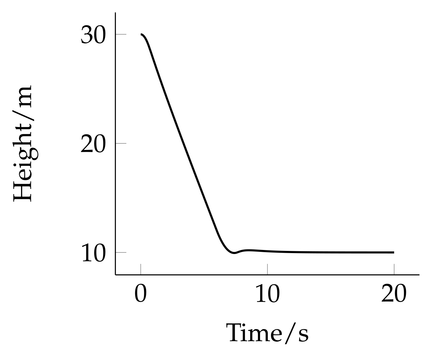
It can be seen that the quadrotor can rise stably and smoothly. Similarly, the command “down 20” is executed at a height of 30, and the height change is as shown in Figure 14.

As can be seen from Figure 14, although there is a slight shock, the land of the drone is still relatively stable.

Horizontal movement has similar control results. Assume that the quadrotor is flying to the right, executing “right 10”. The quadrotor’s X-axis position changes, and the attitude angle changes with time, as shown in Figure 15 and Figure 16.

During the right flight, the quadrotor first tilts to the right to accelerate, and then turns left to slow down and stop. For a quadrotor, the forward, left, and rear directions are all similar to the right, ergo there is no requirement to go into detail.

It can be seen from the above cases that in this model, the quadrotor can fly well under control without weather conditions and can reach the target position.

Model Control Effect under Weather Influencing Factors

First, we test that if the quadrotor will stabilize in a certain position in the event of a sudden wind. Assume that when the quadrotor is stationary in a state of no wind, wind from the rear with a speed of 8 m/s occurs. Influenced by the wind, the quadrotor’s position and attitude change as shown in Figure 17 and Figure 18.

It can be seen that the position of the quadrotor returns to its previous position under a slight disturbance. In terms of attitude, the pitch angle of the quadrotor finally stabilizes at a positive value after the appearance and callback to resist the thrust brought by the wind. The peak in the attitude angle image in Figure 18 must exist, otherwise the quadrotor cannot eliminate the cumulative error in the position.

Figure 19 shows the quadrotor’s movement when it begins to move in the northeast 45° (positive x-axis and positive z-axis) and a sudden wind occurs from the quadrotor’s left.

Figure 20 shows the quadrotor’s movements when the quadrotor moves in the northeast 45° (positive x-axis and positive z-axis) for 2 s and a different sudden wind occurs from the quadrotor’s left.

The following shows the effect of air density on the quadrotor’s flight. Under different air densities, the quadrotor rises 10 m by the same command, and its height changes with time as shown in Figure 21.

In summary, the model can perform stable flight under the influence of environmental factors, and can well demonstrate the difference in the movement of the quadrotor under the influence of environmental factors.

6. Conclusions

We developed a Unity3D-based quadrotor dynamic simulation component on the original simulation platform. Based on Newtonian mechanics and Euler angles, the physical model is established. The model performs a fixed-point control for the simulation. We also introduced weather impact factors into the model through an environmental computational model. The model worked well, and realistically simulated the quadrotors’ motion under many situations.

We believe our simulation component could be useful in the IoT area. A quadrotor, used as a sensor or data collector, is an important part in edge computing. Our simulation model can be used to improve controlling logic or stability of quadrotors, whether they are controlled by operators or self-controlled.

In the future, we will introduce more environmental factors into our model. For instance, how a quadrotor will be affected in a small space and where the airflow made by a quadrotor itself can not be ignored. In addition, in such a small space, how quadrotors will affect each other is another topic worth researching.

References

- Gaponov, I.; Razinkova, A. Quadcopter design and implementation as a multidisciplinary engineering course. In Proceedings of the IEEE International Conference on Teaching, Assessment, and Learning for Engineering (TALE), Takamatsu, Japan, 8–11 December 2012. [Google Scholar]
- Gyrosucer by Keyence. Available online: https://www.oocities.org/bourbonstreet/3220/gyrosau.html (accessed on 7 April 2021).
- Al-Khafajiy, M.; Baker, T.; Hussien, A.; Cotgrave, A. UAV and Fog Computing for IoE-Based Systems: A Case Study on Environment Disasters Prediction and Recovery Plans. In Unmanned Aerial Vehicles in Smart Cities; Springer International Publishing: Cham, Switzerland, 2020; pp. 133–152. [Google Scholar]
- Huo, Y.; Lu, F.; Wu, F.; Dong, X. Multi-Beam Multi-Stream Communications for 5G and beyond Mobile User Equipment and UAV Proof of Concept Designs; IEEE: Piscataway, NJ, USA, 2019. [Google Scholar]
- Marchese, M.; Moheddine, A.; Patrone, F. IoT and UAV Integration in 5G Hybrid Terrestrial-Satellite Networks. Sensors 2019, 19, 3704. [Google Scholar] [CrossRef] [PubMed] [Green Version]
- Google Plans Drone Delivery Service for 2017. Available online: https://www.bbc.com/news/technology-34704868 (accessed on 20 December 2021).
- Ren, Z.; Li, H.; Zhao, Y.; Di, Z. The study of wind resistance testing equipment for unmanned helicopter. In Proceedings of the Advanced Information Technology, Electronic & Automation Control Conference, Chongqing, China, 25–26 March 2017. [Google Scholar]
- Chen, J. Research on Quado-Rator UAV Dynamics Modelling and Controlling Technology. Master’s Thesis, Nanjing University of Science and Technology, Nanjing, China, 2016. [Google Scholar]
- Li, J. Research on Adaptive Inverse Control of a Small Scale Unmanned Quad-rotor Helicopter. Master’s Thesis, Shanghai Jiao Tong University, Shanghai, China, 2014. [Google Scholar]
- De Jesus Rubio, J.; Humberto, P.; Zamudio, Z.; Salinas, A.J. Comparison of two quadrotor dynamic models. IEEE Lat. Am. Trans. 2014, 12, 531–537. [Google Scholar] [CrossRef]
- Wu, X. Research on Flight Control System of Quadrotor UAV. Master’s Thesis, Dalian University of Technology, Dalian, China, 2018. [Google Scholar]
- Masse, C.; Gougeon, O.; Nguyen, D.T.; Saussie, D. Modeling and Control of a Quadcopter Flying in a Wind Field: A Comparison between LQR and Structured ∞ Control Techniques. In Proceedings of the 2018 International Conference on Unmanned Aircraft Systems (ICUAS), St. Dallas, TX, USA, 12–15 June 2018. [Google Scholar]
- Das, A.; Subbarao, K.; Lewis, F. Dynamic inversion of quadrotor with zero-dynamics stabilization. In Proceedings of the IEEE International Conference on Control Applications, San Antonio, TX, USA, 3–5 September 2008. [Google Scholar]
- Quan, Q. Introduction to Multicopter Design and Control; Springer: Berlin/Heidelberg, Germany, 2017. [Google Scholar]
- Khan, W.; Nahon, M. A propeller model for general forward flight conditions. Int. J. Intell. Unmanned Syst. 2015, 3, 72–92. [Google Scholar] [CrossRef]
- Fernando, H.; De Silva, A.; De Zoysa, M.; Dilshan, K.; Munasinghe, S. Modelling, simulation and implementation of a quadrotor UAV. In Proceedings of the 2013 IEEE 8th International Conference on Industrial and Information Systems, Kandy, Sri Lanka, 17–20 December 2013; pp. 207–212. [Google Scholar]
- Tran, N.K.; Bulka, E.; Nahon, M. Quadrotor control in a wind field. In Proceedings of the International Conference on Unmanned Aircraft Systems, Denver, CO, USA, 9–12 June 2015. [Google Scholar]
- Quan, Q.; Dai, X. Flight Evaluation. Available online: https://flyeval.com (accessed on 15 April 2021).
- Zhai, Y.J.; Lin, Z.Y. Design of Software-Defined-Satellite-based PID Attitude Control Application in Python. In Proceedings of the 2018 IEEE 4th Information Technology and Mechatronics Engineering Conference (ITOEC), Chongqing, China, 14–16 December 2018; pp. 133–137. [Google Scholar]
- WebGL: 2D and 3D Graphics for the Web. Available online: https://developer.mozilla.org/en-US/docs/Web/API/WebGL_API (accessed on 23 June 2021).
- Unity Real-Time Development Platform. Available online: https://unity.com (accessed on 23 June 2021).
Figure 1.
This is the schematic diagram of the force of the quadrotor from the top view. The four rotors rotate in different directions.
Figure 2.
This is the schematic diagram of the force of the quadrotor from the side view which shows the force of the quadrotor in a tilted state. It can be seen that the point of application of the upward lift provided by the rotors is obviously not at the geometric center of the quadrotor.
Figure 3.
Schematic diagram of typical MVC (Model View Controller) architecture.
Figure 4.
Data flow diagram. The dotted line indicates that the relevant tasks are completed by the Unity engine.
Figure 5.
Design of the control model and physical model. Formulas deducted in Section 3 are used to control the quadrotor’s attitude and action under specific weather conditions.
Figure 6.
Schematic diagram of quadrotors distance range (top view).
Figure 7.
The new range (top view).
Figure 8.
Target position of the camera (top view).
Figure 9.
Calculating the flow of the environment model.
Figure 10.
Comparison of movement of quadrotors (top view). The right quadrotor is affected by the west wind. The two quadrotors have the same target position.
Figure 11.
Quadrotors affected by a sudden wind (top view).
Figure 12.
Quadrotors affected by air density.
Figure 13.
The quadrotor goes upward.
Figure 14.
The quadrotor goes downward.
Figure 15.
Horizontal position changes when flying to the right.
Figure 16.
Roll angle changes when flying to the right.
Figure 17.
Position changes caused by wind.
Figure 18.
Attitude changes caused by wind.
Figure 19.
Flight under the influence of different side wind speeds.
Figure 20.
Flight when wind speed changes.
Figure 21.
Flight in different air densities.