Processing at the Edge: A Case Study with an Ultrasound Sensor-Based Embedded Smart Device

Abstract

In the current context of the Internet of Things, embedded devices can have some intelligence and distribute both data and processed information. This article presents the paradigm shift from a hierarchical pyramid to an inverted pyramid that is the basis for edge, fog, and cloud-based architectures. To support the new paradigm, the article presents a distributed modular architecture. The devices are made up of essential elements, called control nodes, which can communicate to enhance their functionality without sending raw data to the cloud. To validate the architecture, identical control nodes equipped with a distance sensor have been implemented. Each module can read the distance to each vehicle and process these data to provide the vehicle’s speed and length. In addition, the article describes how connecting two or more CNs, forming an intelligent device, can increase the accuracy of the parameters measured. Results show that it is possible to reduce the processing load up to 22% in the case of sharing processed information instead of raw data. In addition, when the control nodes collaborate at the edge level, the relative error obtained when measuring the speed and length of a vehicle is reduced by one percentage point.

1. Introduction

Intelligent systems, based on embedded devices, have been the focus of attention in intelligent city environments. The use of cheap and efficient micro-controllers with high connectivity features allows the devices’ integration into almost all types of urban elements. These interconnected elements have given rise to the concept of the Internet of Things (IoT) [1]. Having many distributed devices implies a large amount of data to manage to obtain information to make some decisions. This distributed chain, sensor-decision-act, is aimed to provide an optimisation of system performance and to provide optimal services [2]. This optimisation has given rise to the concept of distributed intelligence, usually based on distributed knowledge [3].

Among the fields of application of distributed intelligence, mobility environments, both in cities and on roads, are one of the most widely used. Environments can apply intelligence in everyday aspects such as optimising traffic or managing the power consumption of road lighting [4]. Using embedded systems with distributed intelligence to coordinate non-daily aspects, such as accident prevention, detection or management, is also a challenge. In all cases, intelligent environment management requires devices to detect, characterise, predict, or act on the behaviour of both elements—vehicles and pedestrians. Beyond intelligent devices appears the concept of collaborative intelligence in the edge based on the connection between close devices. For example, if some streetlights can detect vehicles, they can alert traffic lights about their characteristics such as size or speed. With this information, traffic lights can adjust the time they will stay green or red to minimise the waiting time for vehicles. For example, several streets can send enough information to provide a picture of the traffic in an area and to be able to predict traffic congestion situations intelligently.

There are many methods of detecting and characterising vehicles on roads. The most efficient methods use complex devices, such as cameras [5] or even drones [6]. These devices can be tempting for vandalism, in addition to not having the availability of a high processing or communicating capacity [7]. As an alternative to the previous systems, cheap solutions have been proposed. The use of simple sensors implies that the information provided by complex sensors, such as cameras, must be supplied through intelligence. In [8], two classes of neural networks are considered, multi-layer perceptron (MLP) and convolutional neural network (CNN), to analyse the audio signal.

To implement intelligence within embedded devices, we use a minimum element called a ’control node’ (CN). A control node is an element that can read from sensors and write to actuators, or both. The core of a control node is a micro-controller with communication capabilities that must perform basic processing of the data obtained from the sensors. Consequently, the computational and communication capabilities embedded into the CNs implies that a set of CNs can provide an intelligent distributed system.

In this context, an interesting question emerges: Is it worth distributing if a single CN can provide an acceptable result? If CNs distribute their raw data, the messages load the communications system. A high load of messages implies a high probability of errors such as high latency or variable jitter, among others. Moreover, an increased communication load implies that the CN must handle more incoming and outgoing messages. Due to the limited computational resources of the CN, an increase in communication activity can limit the micro-controller resources dedicated to computational algorithms. To answer the previous question, it is necessary to know the processing response time that a CN could provide, considering both control and communication processing requirements. The measurement of this response time will involve knowing the reaction times and how the action or information provided is adequate to the requirements. For example, in the experiment presented in this article, a concrete CN is used to measure the speed of a vehicle using an ultrasound sensor. A single sensor has a considerable error; however, if the system has multiple sensors, it is possible to improve the accuracy of the measurement by distributing the data from each CN.

This article proposes a distributed paradigm where the control nodes (CN) have intelligence dedicated to a specific functionality. Only the relevant data are distributed instead of classical hierarchical models where the CN are only raw data providers. The article depicts how the CN works as the primary element based on this paradigm. Additionally, the article describes how connecting two or more CN, forming an intelligent device, can improve the accuracy of the parameters measured. We developed a smart device that detects vehicles’ speed and length. Different CNs compound the intelligent devices. Each CN has an ultrasonic (US) sensor that detects distance. Changing the ultrasound signal’s emission angle makes it possible to accurately detect the vehicle speed or length.

The experiments measured the data processing time (to obtain distances) and the processing time to generate the information (speed and length). The results show that reducing the overall processing time is possible if the modules undergo previous processing and provide information to other modules instead of providing the raw data. This article has been organised as follows. The following section shows the proposed paradigm from the classical pyramid to the inverted pyramid. Additionally, as the CN is the basis of the architecture, we provide a CN description and characterisation to measure the optimisation experiment. Section 3 presents the case study consisting of a device composed of three CN modules with an ultrasound sensor at each one. In addition to acquiring distances, these CN modules can process and calculate both vehicle speed and length. Section 4 presents a CN module simulation to have a proof of concept. Section 5 presents the experiments made with a device with two different CN modules configurations. In the first case experiment, two CN modules send the raw distance data to a third CN module dedicated to calculating the vehicle speed and length in the first case. In the second case, each CN module processes its data and produces a candidate speed value. The speed value is transmitted to the third CN module that obtains the vehicle length. Finally, the article ends with the conclusions and possible studies to be carried out in future research.

2. Background and Related Work

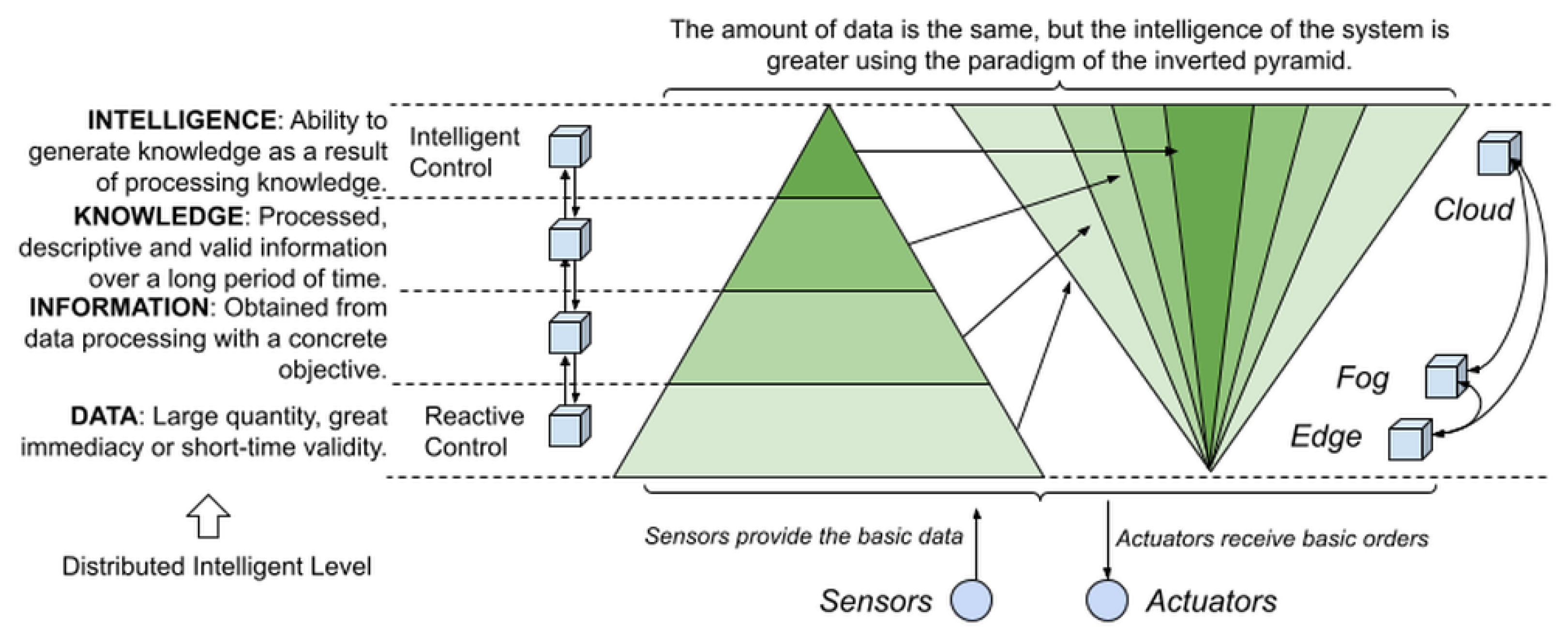
2.1. Placing Elements at Different Levels

This subsection shows the shift between the intelligent hierarchical control pyramid and how embedded devices generate a new inverted pyramid model [9]. The vision of the ’pyramid of knowledge’ in intelligent control systems implies an analogy with the CN of each level (Figure 1). A description and review of such a pyramid can be obtained in [10]. The data source (pyramid base) is the sensors that provide raw data representing physical values measured by parameters. Raw data are processed to obtain basic information. For example, a series of isolated temperature measurements can provide an average value and error or a trend in temperature change. The processed information can produce knowledge. For example, different temperature oscillations over several days can estimate the existing climate. Finally, the knowledge is used to generate intelligence. For example, knowledge of the climate in a location allows predicting changes and taking preventive action. This process is known as learning and is the basis of advanced machine learning methods.

At the low level of the pyramid, the primary data characteristic is the short period in which the data are valid. For example, a vehicle detection sensor will report the vehicle presence at a specific time moment and in a particular place. As the elements of the system grow, specifically in lower layers of the classical pyramid (i.e., a large number of CNs), a considerable amount of data is available. Many connected elements that provide this massive data have led to the emergence of the Internet of Things (IoT) or Industry 4.0 paradigm. Including the IoT and Industry 4.0 paradigm in distributed intelligent systems implies reviewing the knowledge pyramid, such as the one proposed in [11]. Currently, there is a consensus to divide distributed systems in a layer close to the physical environment (fog, edge in the hardware) and cloud to provide massive data processing, advanced computing or machine learning. These layers (or ’areas’) have changed the design of system architectures, forcing a turn away from the hierarchical models towards highly connected horizontal models. In these new models, intelligence becomes distributed and not exclusively at the top of the classic pyramid of knowledge model (Figure 1). Consequently, a system architecture must support intelligence at the edge level but provide all available data to the cloud level. Edge elements, as CNs, can provide some intelligent processing that helps fog and cloud obtain the data processed and avoid the fog and cloud elements from making decisions that a CN can make.

This process is known as edge computing and is a concept linked to the emergence of the Internet of Things [12]. Edge computing is performed by devices in direct contact with the data source or sensors allowing more direct communication between devices. This article is about devices where sensors that require simple computation, such as infrared or ultrasonic, can provide relevant information. The use of these devices is useful in a lot of scenarios, mainly dedicated to road safety [13]. To achieve this security, it is necessary to be able to detect and characterise aspects such as speed or type of vehicle through the use of sensors. Most detection and characterisation systems use a combination of different types of sensors. For example, infrared and ultrasonic are used in [14]. It is also possible to use only one type of sensor for speed detection. In the case of [15], speed detection is based on ultrasonic sensors to detect speed violations. Based on the previous work, the next subsection presents the analysis of these types of devices.

2.2. Control Node Characterisation at the Edge Level

It is necessary to measure the time spent to control processing and communication tasks to compare the performance of a single CN and a set of CNs working collaboratively. Figure 2 broadly shows the times involved in control and communication actions inside a single CN. The inputs of a CN are the communications ’Comm’ that receive service requests from other CN or upper elements and the sensor data provided by the corresponding hardware elements. In turn, the outputs of the CN are the communications ’Comm’ services to other edge nodes or system elements (cloud or fog) and the actuators ’Hw (actuators)’.

In this context, a CN can have different configurations. A CN without incoming or outgoing communications is an autonomous reactive node; it is not usual, but there are, for example, irrigation systems without remote monitoring or configuration. A CN that only senses is the basis of distributed wireless sensor networks (WSN), systems widely used in human environments [16]. In the same way, a CN without sensors and actuators also does not make sense in the context of distributed control.

Regardless of the configuration used in a CN, one must measure its performance to understand its ability to assimilate some intelligent algorithms. Absolute and relative errors measure the efficiency of the control action. Low error values imply effective control, even though the processing and the communications load can amount to 100% of micro-controller use. Consequently, high efficiency could mean high electricity consumption [17]. Therefore, the cost of such efficiency may be higher than the efficiency achieved. However, for a CN, or set of CNs, the goal is to obtain a low response time and low micro-controller processing load, in addition to common error values. Thanks to data processing, the control error can be decreased from other CN. In that case, it is convenient to evaluate whether it is efficient to wait for the remote data or to act locally with a more significant error. When a CN must communicate through a shared communications system, you have a distributed system. In this case, in addition to the times considered in Figure 2, the times invested in the communication tasks between nodes should be considered as an integral part of the CN response time. Figure 3 shows all times involved due to the use of connected CN devices.

The times involved in this case depend on the system architecture. When nodes are on the edge or fog, in other words, they share a communication medium, these times are usually shorter than the times involved in cloud communication. From times outlined in Figure 3, depending on the system errors, it is possible to customise from a CN to a distributed intelligent system to spend optimal time to pre-process data. The following section will use these times to characterise a simple system and check which formulas can answer whether it is better to act fast with a specific error or wait a while to act but with a minor absolute or relative error.

3. The Proposed Solution

This section presents a case study based on an intelligent device consisting of a smart device with some CN modules. The aim of the device tested is to measure the speed and the length of a vehicle based on the work presented in [18].

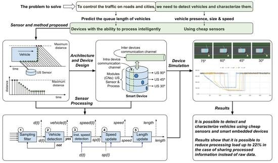
3.1. Vehicle Detection and Characterisation Method

The way to measure vehicle speed and length is to compare different distance measurements of a vehicle as it approaches the US sensor. Figure 4a shows how a sensor with an inclination of 45° to the road axis can detect the front and side of a vehicle. These distance measurements are the maximum possible when no vehicle is present. The distance measurement becomes a downward ramp when the front of a vehicle is detected. Next, the measurement becomes a constant distance as soon as the side is detected. Finally, when the vehicle disappears, the measurement becomes the maximum possible again.

The device consists of three interconnected CNs. The CN has been built from the JSN-SRT04 ultrasonic (US) sensor module. This US sensor is waterproof and widely used in industry, mainly for measuring the liquid tank level or the distance between elements in outdoor environments [19]. The sensor has a detection range from 0.20 to 6 m. This range makes it suitable for covering both road and street lane vehicle profiles. The resolution of the distance is 0.01 m, so it allows relevant variations of vehicle distance so that the detection algorithm can work efficiently. The relative error detected in the measurements is 0.74% on average [20] with a linear relation between distance and error [21]. The sensor sampling rate used in the device was 500 KHz in the experiments. The sensors have been connected to an Arduino Nano, which communicates with the device’s CNs via an Inter-Integrated Circuit (I2C). This channel allows serial communication between a master and several slaves at speeds between 100 Kbits/s and 3.4 Mbits/s [22]. I2C is a channel widely used in embedded systems due to its simplicity to manage it. Figure 4b shows the experimental device. This experimental device has three modules or CNs. Each of them has a specific orientation. Depending on the orientation angle in which the ultrasound sensor is tilted concerning the road’s longitudinal axis, there is a specific distance profile along the time for each detected vehicle. The different orientations can obtain a different measurement profile over time. Figure 5 shows the three measurement profiles with US sensors oriented to 30°, 45° and 90°. Below each module orientation, the signal profile obtained from distance over time is shown. With the module oriented at 30° degrees, the number of samples in which the vehicle’s front cuts the US ray is greater than with the module oriented at 45° degrees. Comparing the 30° and 45° degree modules, the 30° modules can obtain a more accurate calculation of speed. As the 90° module cannot detect the front of the vehicle, it can only estimate the length of the vehicle measuring its side. Therefore, the 90° module cannot calculate the vehicle speed directly. As long as the 90° module has a speed value from another CN, it can calculate the length of the vehicle crossing in front of its US sensors.

Each of the CNs for the device shown in Figure 5 is similar and depend on their orientation to provide speed or distance with concrete accuracy. When a vehicle has been detected, the module calculates the vehicle’s speed based on the change between the front and side of the vehicle. When the sensor returns to provide the maximum distance, it is considered that the transition of the vehicle has already been completed.

3.2. Vehicle Detection and Characterisation Process

The processes that a module performs to detect and characterise a vehicle are shown in Figure 6. As shown in this figure, a module that acts as a CN can detect a vehicle and determine its speed, as well as the length of it.

As previously discussed, Figure 4 illustrates how vehicle detection is initiated when the sensor starts to detect a distance less than the maximum distance determined. Consequently, the first step is to sample and filter the data, because the ultrasound signal is subject to many problems, including echoes and material-dependent responses. This first step (1 in Figure 4) consists of sampling five distances and calculating their average to obtain the main data, distance $d\left(t\right)$. Not all samples are correct, for example, echoes can produce false measurements. The raw data are filtered to identify any values that could lead to erroneous measurements. Filtering is performed by discarding the samples that do not comply with the sensor minimum and maximum constraints or that differ by 10% from a window of five previous samples. Additionally, if the filter detects two continuous erroneous samples, five-window samples are discarded. In the second phase (2 in Figure 4), the vehicle is detected. Vehicle detection occurs when the values $d\left(t\right)>d(t+1)$ over N consecutive operation cycles. Initially, N is set to two. In order to characterise both the spatial and kinematic properties of a vehicle during its detection phase, a non-parametric method called frame differences [23] is required. The spatial characteristics of the vehicle are its length, while the kinematic characteristic is its speed. The module changes to instantaneous speed detection when an approaching vehicle has been detected (phase 3 in Figure 4). During instantaneous detection, the speed is calculated by comparing the two distances obtained by consecutive measurements of the vehicle’s front. Since the difference of distances detected and time between these distances is available, the vehicle speed calculation is immediate. From the instantaneous speed detected, the fourth phase (4, in Figure 4) updates the speed value. As a result of this update, an average speed and standard deviation can be detected. Additionally, this phase can recognise specific patterns, such as acceleration and deceleration of the vehicle. When the difference between two consecutive distances is less than a certain threshold, 5% in the experiments, the side of the vehicle is considered detected. From this point on-wards, the length update phase, 5 in Figure 4, starts. Based on the speed calculated in the previous phase, this phase works while the vehicle is being detected to determine the vehicle length. According to the needs of other control nodes, the control node can send them raw or processed data. This aspect allows CNs to decrease their process load but increases the network throughput. Due to this, all phases can offer their outputs to other control nodes (phase 6 in Figure 4).

4. Experiments and Results

As explained in the previous sections, one of the goals of edge computing is to determine whether the ratio of processing load to the accuracy of the result is acceptable. In light of this, checking the processing and communication load for different device configurations is essential. To test all previous concepts, we have developed a device with several modules, each of which is a CN. The experimentation has been carried out in two phases: simulation and prototyping. The simulation has been performed on the measurement accuracy of a single CN with a US sensor. The simulation aimed to determine which angles are the most appropriate to be implemented in a prototype. Based on the simulation results, the prototyping performed consists of a single device, using three different CNs with the US sensor oriented with the angles: 30°, 45°, and 90°, as described in Figure 5.

4.1. Simulations

The simulation has been carried out using the simulator presented in [24] and coded in Python. Based on the Pygame environment [25], we extend the simulator code to introduce the CN with a US sensor. The experimental environment consists of an entry vehicle with a fixed speed that can be varied to generate different cases. A US sensor that allows the entry angle to be varied is also included. This US sensor detects the distance between the sensor exit ray and the collision point in the vehicle. The vehicle simulated has a size of 100 cm for the front and 180 for the side. A constant speed of 2.25 m/s is applied to the vehicle. Figure 7 shows the sensor with different angles and the corresponding data collected of the distances.

As can be seen in Figure 7, the angles closer to the road axis obtain a more significant amount of data from the front of the vehicle. This amount of data means that more possible speeds are available, which generates a minor relative error in the calculation.

Table 1. Simulation data obtained. Average of the valid samples in the detection of the front and side of the vehicle and calculated speed, together with the corresponding errors.

	90°	75°	60°	45°	30°
Samples front	-	12	25	44	76
Samples side	84	83	83	82	81
Calculated Speed	-	2.06 m/s	2.16 m/s	2.20 m/s	2.22 m/s
Relative Error	-	8.44%	4.00%	2.22%	1.33%

shows the parameters obtained from simulating five vehicles with the same characteristics for each angle.

From the simulation data, it seems appropriate to use control modules with angles close to the road axis. Consequently, angles of 30° and 45° are selected for experimentation on the prototype. The length calculation is based on the lateral samples. In all cases, the number of samples is similar, although the shortest distances are obtained with the angles perpendicular to the road axis, i.e., with the angles of 75° and 90°. Since the 75° speed error is the largest, it seems appropriate to use only one sensor at 90° for the calculation of the vehicle length.

4.2. Prototyping

A vehicle with a length of 3.7 m was used for the experiment. The vehicle has been passed through the measuring module ten times for angles of 30°, 45° and 90°. For each angle, the vehicle speed was 10 m/s (36 km/h). Measured times are all in milliseconds (ms). The device aims to measure the vehicle speed and length accurately. To achieve this accuracy, the CNs must collaborate among them. The modules configured with 30° and 45° can obtain vehicle speed accurately. The module configured with 90° can obtain the vehicle length using the speed obtained from the previous angled CNs. Two different cases have been tested. The first case represents central processing and the second case represents distributed processing. In the first case, the 30° and 45° modules transmit the raw data of the measured distances to the 90° module. This case corresponds to a hierarchical model in which the angled CNs are dedicated to data collection. In contrast, the 90° node is dedicated to collecting data and calculating the resulting speed and length. Results are shown in

Table 2. Results obtained from two control nodes (CN30 and CN45) sending raw data to the third module (CN90).

	CN30	CN45	CN90
tControl(AVG)	32.34 ms	28.97 ms	235.73 ms
tControl (STD)	3.85 ms	2.15 ms	18.93 ms
tResponse (AVG)	51.38 ms	31.38 ms	276.54 ms
tResponse (STD)	3.18 ms	2.18 ms	20.49 ms
tLatency (AVG)	1340.81 ms	1362.25 ms	-
tLatency (STD)	90.90 ms	87.34 ms	-
Speed (AVG)	-	-	10.12 m/s
Speed (STD)	-	-	1.17 m/s
Speed (Rel.E)	-	-	5.79%
Length (AVG)	-	-	3.76 m
Length (STD)	-	-	0.15 m
Length (Rel.E)	-	-	1.61%

.

In the second case, the 30° and 45° degrees CNs calculate the speed and length average, in conjunction with the standard deviation, and this information is sent to the 90° degree module. Results are shown in

Table 3. Results were obtained from the three CNs processing data and sharing the information obtained. The third module (CN90) uses the speeds calculated by the modules CN30 and CN45 to calculate the vehicle length and the vehicle speed.

	CN30	CN45	CN90
tControl(AVG)	45.51 ms	49.65 ms	113.04 ms
tControl (STD)	5.34 ms	1.44 ms	1.06 ms
tResponse (AVG)	105.16 ms	56.67 ms	132.22 ms
tResponse (STD)	1.77 ms	4.77 ms	12.06 ms
tLatency (AVG)	1339.41 ms	1362.65 ms	-
tLatency (STD)	92.30 ms	85.94 ms	-
Speed (AVG)	10.55 m/s	12.92 m/s	10.08 m/s
Speed (STD)	1.01 m/s	1.18 m/s	0.97 m/s
Speed (Rel.E)	5.79%	17.77%	4.12%
Length (AVG)	-	-	3.71 m
Length (STD)	-	-	0.09 m
Length (Rel.E)	-	-	0.78%

.

5. Discussion

The results obtained show how the speed and length calculated by the CN90 module have similar accuracy to the previous case. This result is expected but is not the aim of the experiment. We need to compare the total time involved in both cases. If we calculate the overall time that the device dedicates to the process, we obtain 315.04 ms in the first case, but the total process time is 208.00 ms in the second case.

Indeed, if we consider the response time, thus it is the sum of communications and process times, the results are 359.3 ms in the first case and 294.05 ms in the second one. This result means that distributed processing saves around 22% of processing and communications time. The results show how distributing the processing between CNs in the device decreases the overall processing time. Although the latency time has no significant changes, since modules work in an I2C network, there is considerable data transferred in the first case. Due to this, five messages must be sent with the measured distances for each message with the instantaneous speed transmitted. This difference is even more significant in the case of transmitting only the final speed or the final transmitted length.

Reducing messages and processing data before sending it has relevant implications, especially for power consumption due to the processing time and network load. The power consumption has been measured, at the module level, in order to check the energy savings. The three modules implied in the first case have a total consumption average of 0.5269 W per second, whereas the second case has a total consumption of 0.5141 W per second. The difference in consumption is small because communications are a major part of the time consumed. However, processing consumption is relevant. This indicates the importance of optimising processing to reduce communications.

6. Conclusions

This article has presented a paradigm that allows modules to share data and process information. Based on the paradigm presented, a module called a control node (CN) has been presented and characterised. A CN has been implemented as part of a device that obtains the speed and the length of vehicles using ultrasonic sensors. These low-cost and high-error sensors provide data that improve the accuracy of the devices that receive this information instead of raw data being processed and distributed as a piece of information. It is possible to prove how the collaboration of modules at the edge level improves the quality of the information, measured in terms of the relative error.

Experiments have proven that processing data close to the CN reduces the overall time dedicated to processing in global terms. These results open the door to future experiments where information is shared through the fog between devices in addition to sharing information within a device. The overall power consumption of the system can be reduced. This reduction implies that studying how to process data close to the edge level is a good starting point for new experiments. Additionally, some parameters can be used to tune the system. Aspects such as message transmission policy based on the relative error to reduce non-relevant information can optimise the system performance. As a future research line, we propose implementing CN as cells of a distributed neural network that, dynamically, can select which kind of information suits to be distributed.

References

1. Xia, F.; Yang, L.T.; Wang, L.; Vinel, A. Internet of things. Int. J. Commun. Syst. 2012, 25, 1101. [Google Scholar] [CrossRef]
2. Amurrio, A.; Azketa, E.; Javier Gutierrez, J.; Aldea, M.; Parra, J. A review on optimization techniques for the deployment and scheduling of distributed real-time systems. Rev. Iberoam. Autom. Inform. Ind. 2019, 16, 249–263. [Google Scholar] [CrossRef]
3. Zare, R.N. Knowledge and distributed intelligence. Science 1997, 275, 1047–1048. [Google Scholar] [CrossRef]
4. Poza-Lujan, J.L.; Sáenz-Peñafiel, J.J.; Posadas-Yagüe, J.L.; Conejero, J.A.; Cano, J.C. Use of Receiver Operating Characteristic Curve to Evaluate a Street Lighting Control System. IEEE Access 2021, 9, 144660–144675. [Google Scholar] [CrossRef]
5. Sun, Z.; Bebis, G.; Miller, R. On-road vehicle detection using optical sensors: A review. In Proceedings of the 7th International IEEE Conference on Intelligent Transportation Systems (IEEE Cat. No. 04TH8749), Washington, WA, USA, 3–6 October 2004; pp. 585–590. [Google Scholar]
6. Li, W.; Li, H.; Wu, Q.; Chen, X.; Ngan, K.N. Simultaneously detecting and counting dense vehicles from drone images. IEEE Trans. Ind. Electron. 2019, 66, 9651–9662. [Google Scholar] [CrossRef]
7. Lozano Dominguez, J.M.; Mateo Sanguino, T.J. Review on V2X, I2X, and P2X Communications and Their Applications: A Comprehensive Analysis over Time. Sensors 2019, 19, 2756. [Google Scholar] [CrossRef] [PubMed] [Green Version]
8. Golovnin, O.; Privalov, A.; Stolbova, A.; Ivaschenko, A. Audio-Based Vehicle Detection Implementing Artificial Intelligence. In International Scientific and Practical Conference in Control Engineering and Decision Making; Springer: Berlin/Heidelberg, Germany, 2020; pp. 627–638. [Google Scholar]
9. Poza-Lujan, J.L.; Uribe-Chavert, P.; Sáenz-Peñafiel, J.J.; Posadas-Yagüe, J.L. Distributing and Processing Data from the Edge. A Case Study with Ultrasound Sensor Modules. In International Symposium on Distributed Computing and Artificial Intelligence; Springer: Berlin/Heidelberg, Germany, 2021; pp. 190–199. [Google Scholar]
10. Körner, M.F.; Bauer, D.; Keller, R.; Rösch, M.; Schlereth, A.; Simon, P.; Bauernhansl, T.; Fridgen, G.; Reinhart, G. Extending the automation pyramid for industrial demand response. Procedia CIRP 2019, 81, 998–1003. [Google Scholar] [CrossRef]
11. Jennex, M.E. Big data, the internet of things, and the revised knowledge pyramid. ACM SIGMIS Database 2017, 48, 69–79. [Google Scholar] [CrossRef]
12. Shi, W.; Dustdar, S. The promise of edge computing. Computer 2016, 49, 78–81. [Google Scholar] [CrossRef]
13. Hadi, S.N.; Murata, K.T.; Phon-Amnuaisuk, S.; Pavarangkoon, P.; Mizuhara, T.; Jiann, T.S. Edge computing for road safety applications. In Proceedings of the 2019 23rd International Computer Science and Engineering Conference (ICSEC), Phuket, Thailand, 30 October–1 November 2019; pp. 170–175. [Google Scholar]
14. Odat, E.; Shamma, J.S.; Claudel, C. Vehicle classification and speed estimation using combined passive infrared/ultrasonic sensors. IEEE Trans. Intell. Transp. Syst. 2017, 19, 1593–1606. [Google Scholar] [CrossRef]
15. Liu, J.; Han, J.; Lv, H.; Li, B. An ultrasonic sensor system based on a two-dimensional state method for highway vehicle violation detection applications. Sensors 2015, 15, 9000–9021. [Google Scholar] [CrossRef] [PubMed] [Green Version]
16. Mendoza Merchán, E.V.; Benitez Pina, I.F.; Núñez Alvarez, J.R. Network of multi-hop wireless sensors for low cost and extended area home automation systems. RIAI-Rev. Iberoam. Autom. Inform. Ind. 2020, 17, 412–423. [Google Scholar]
17. D’Andrea, R.; Dullerud, G.E. Distributed control design for spatially interconnected systems. IEEE Trans. Autom. Control. 2003, 48, 1478–1495. [Google Scholar] [CrossRef] [Green Version]
18. Hernández Bel, A. Dispositivo Modular Configurable para la Detección de Vehículos, y Viandantes, y con Soporte a la Iluminación de la Vía e Información de Tráfico. Master’s Thesis, DISCA, UPV, Valencia, Spain, 2020. [Google Scholar]
19. Panagopoulos, Y.; Papadopoulos, A.; Poulis, G.; Nikiforakis, E.; Dimitriou, E. Assessment of an Ultrasonic Water Stage Monitoring Sensor Operating in an Urban Stream. Sensors 2021, 21, 4689. [Google Scholar] [CrossRef] [PubMed]
20. Andang, A.; Hiron, N.; Chobir, A.; Busaeri, N. Investigation of ultrasonic sensor type JSN-SRT04 performance as flood elevation detection. In IOP Conference Series: Materials Science and Engineering; IOP: Bandung, Indonesia, 2019; Volume 550, p. 012018. [Google Scholar]
21. Prasetyono, A.; Adiyasa, I.; Yudianto, A.; Agit, S. Multiple sensing method using moving average filter for automotive ultrasonic sensor. In Journal of Physics: Conference Series; IOP: Bristol, UK, 2020; Volume 1700, p. 012075. [Google Scholar]
22. Semiconductors, P. The I2C-bus specification. Philips Semicond. 2000, 9397, 00954. [Google Scholar]
23. Weng, M.; Huang, G.; Da, X. A new interframe difference algorithm for moving target detection. In Proceedings of the 2010 3rd International Congress on Image and Signal Processing, Yantai, China, 16–18 October 2010; Volume 1, pp. 285–289. [Google Scholar]
24. Gandhi, M.M.; Solanki, D.S.; Daptardar, R.S.; Baloorkar, N.S. Smart Control of Traffic Light Using Artificial Intelligence. In Proceedings of the 2020 5th IEEE International Conference on Recent Advances and Innovations in Engineering (ICRAIE), Jaipur, India, 1–3 December 2020; pp. 1–6. [Google Scholar] [CrossRef]
25. McGugan, W. Beginning Game Development with Python and Pygame: From Novice to Professional; Apress: New York, NY, USA, 2007. [Google Scholar]
Figure 1. The different intelligence levels are related to the classic vision of the pyramid of knowledge (left side of the figure) and the relationship with intelligent control (right side of the figure).
Electronics 11 00550 g001
Figure 2. Times related to communications and processing of a single control node (CN).
Electronics 11 00550 g002
Figure 3. Times related to communications between two different control nodes (CN) connected in the fog or the cloud.
Electronics 11 00550 g003
Figure 4. Method to detect the vehicle’s front and side using US rays (a), and the device implemented with US modules (b).
Electronics 11 00550 g004
Figure 5. Selected configurations that provide a reasonably accurate estimation of vehicle characteristics: 30° (a), 45° (b), and 90° (c).
Electronics 11 00550 g005
Figure 6. Phases performed by a module to detect and characterise a vehicle.
Electronics 11 00550 g006
Figure 7. Selected configurations that provide a reasonably accurate estimation of vehicle characteristics: 90°, 75°, 60°, 45°, and 30°, and corresponding distances obtained (bottom).
Electronics 11 00550 g007