TAWSEEM: A Deep-Learning-Based Tool for Estimating the Number of Unknown Contributors in DNA Profiling

Abstract

DNA profiling involves the analysis of sequences of an individual or mixed DNA profiles to identify the persons that these profiles belong to. A critically important application of DNA profiling is in forensic science to identify criminals by finding a match between their blood samples and the DNA profile found on the crime scene. Other applications include paternity tests, disaster victim identification, missing person investigations, and mapping genetic diseases. A crucial task in DNA profiling is the determination of the number of contributors in a DNA mixture profile, which is challenging due to issues that include allele dropout, stutter, blobs, and noise in DNA profiles; these issues negatively affect the estimation accuracy and the computational complexity. Machine-learning-based methods have been applied for estimating the number of unknowns; however, there is limited work in this area and many more efforts are required to develop robust models and their training on large and diverse datasets. In this paper, we propose and develop a software tool called TAWSEEM that employs a multilayer perceptron (MLP) neural network deep learning model for estimating the number of unknown contributors in DNA mixture profiles using PROVEDIt, the largest publicly available dataset. We investigate the performance of our developed deep learning model using four performance metrics, namely accuracy, F1-score, recall, and precision. The novelty of our tool is evident in the fact that it provides the highest accuracy (97%) compared to any existing work on the most diverse dataset (in terms of the profiles, loci, multiplexes, etc.). We also provide a detailed background on the DNA profiling and literature review, and a detailed account of the deep learning tool development and the performance investigation of the deep learning method.

1. Introduction

DNA profiling, or DNA typing, was introduced in 1985 by Jeffreys [1]. Several areas in chromosomal DNA contain repeated DNA sequences. These sequences may differ from one individual to another [1]. Jeffreys found that he could gain vital information about an individual by looking at his or her DNA profile. For example, he was able to know from the DNA profile of a person whether the person was related to another specific individual. Since then, many vital applications of DNA profiling have been introduced. DNA profiling is very challenging because it involves distinguishing two persons using DNAs that are highly similar for all humans [1].

A critically important application of DNA profiling is in the forensic science domain, and is that of criminal investigations. This is the first use of DNA profiling, where it helped to identify the killer of two girls in England in 2008 by finding a match between the killer’s blood sample and the DNA profile found on the crime scene [1]. Another application is the paternity test. Each year in the United States, more than 300,000 paternity tests are performed, where the identity of the father of a child needs to be found. In 2008, almost one million samples were investigated for this purpose [1]. Other important applications of DNA profiling include disaster victim identification, missing person investigations, and mapping genetic diseases [2].

A crucial task in DNA profiling is the determination of the number of contributors in a DNA mixture profile. It could help, for example, in sexual assault cases where the sources of a DNA mixture include multiple individuals, including the victim, the criminal, and perhaps the victim’s partner, a criminal partner, and other individuals. Finding this unknown number of contributors in a DNA mixture profile is challenging due to issues that include allele dropout, stutter, blobs, and noise in DNA profiles. The complexity of the task (finding the number of contributors) increases exponentially with the increase in the number of unknowns in the DNA mixture [2,3,4,5]. This problem is the focus of this paper.

Researchers have attempted to address the problem of finding the number of contributors in a DNA mixture profile. The challenges in this respect include estimating the number of contributors with high accuracy and within reasonable times. The methods that have been developed for the purpose can be divided into three categories: basic methods, high-performance computing (HPC) methods, and machine learning methods [6]. The basic methods rely on techniques such as likelihood ratio estimation and are usually very compute-intensive [7,8]. Various parallel computing (HPC) approaches have been proposed to address the computational complexity of this problem [9,10,11]. The accuracy and computational complexity of the basic and HPC methods still remain a problem [2,11,12,13]. Machine learning methods, as is the case for many application domains, have been applied for estimating the number of unknowns. However, there is limited work in this area, with only four works in total [6]; many more efforts are required in terms of developing highly accurate models and their training on large and diverse datasets (see Section 3 for a detailed review of the relevant works).

With the aim to advance the cutting-edge in this area, in this work, we propose and develop a software tool called TAWSEEM (Tawseem is an Arabic word meaning “labeling” or “tagging”; we imply by this word in our context something that helps to distinguish things from each other, and we named the tool TAWSEEM to show its ability to profile or distinguish DNAs from each other) for estimating the number of unknown contributors in DNA mixture profiles. The tool uses a multilayer perceptron (MLP) neural network model for identifying the number of contributors in DNA mixture profiles. We use the PROVEDIt (Project Research Openness for Validation with Empirical Data) dataset [14] for the purpose of training and validating our deep-learning-based model. The PROVEDIt dataset contains over 25,000 multiplex STR (short tandem repeat) profiles formed from one to five known persons, ranging from simple to complex profiles. This is the largest publicly available dataset of its kind and none of the earlier works have used this dataset in its entirety for DNA profiling (to the best of our knowledge, there is only one work [15] that has reported the use of the PROVEDIt dataset for machine-learning-based methods, but there are a small number (766) of profiles from it). We investigate the performance of our developed deep learning model using four performance metrics, namely accuracy, F1-score, recall, and precision. The deep learning model for the highest number of profiles provides a 97% accuracy for mixtures with five contributors.

The novelty of our research presented in this paper is evident in the fact that the deep learning models have provided the highest accuracy compared to any other related works in the literature, and that these results are achieved on a dataset that is the largest in its size, as well as containing the most diversity (in terms of the profiles, loci, multiplexes (kits), etc.) among all the datasets used in the literature in similar works. Another contribution of this paper is to provide a detailed background on DNA profiling and the literature review. The existing works have not covered background on DNA profiling in such detail: either the background is provided in great detail in books or is scantily covered in research papers. Similarly, some works have reported the literature on DNA profiling [2]: these works are slightly old and none have covered machine-learning DNA profiling methods. Moreover, this paper provides a detailed account of the deep learning tool development and the performance investigation of the deep learning method across various multiplexes, loci, and profiles. Such modeling details and the analysis of results have not been reported in other DNA profiling works.

This work is part of our broader work on DNA profiling. Earlier, we developed the first distributed-memory HPC implementations [11] of DNA profiling using maximum likelihood ratio computations and reported results for up to ten unknowns delivering over 15× the performance using over 3000 cores. In another recent work [6], we investigated the performance of six machine learning algorithms for estimating the number of unknowns on a small subset (780 profiles) of the PROVEDIt dataset without exploring the performance across various multiplexes, loci, and profiles.

This paper is organized as follows. In Section 2, we define and explain the background concepts. In Section 3, we discuss in detail the related works. In Section 4, we provide the methodology and design of our tool. In Section 5, we discuss the results in detail and compare them with the related works. Finally, in Section 6, we conclude and give future directions.

2. Background

This section provides a brief background of the concepts related to DNA profiling. Section 2.1 provides definitions of the gene, alleles, and loci, and explains the difference between the heterozygous and homozygous alleles. Section 2.2 explains what DNA mixtures are and how to decide whether it is a DNA mixture. Section 2.3 explains the genetic markers (loci). Section 2.4 explores the major challenges that will increase the complexity of the DNA profiles. More explanations about the forensic science field and DNA profiling are given in Section 2.5. Section 2.6 explains likelihood estimation, and, finally, Section 2.7 discusses DNA databases.

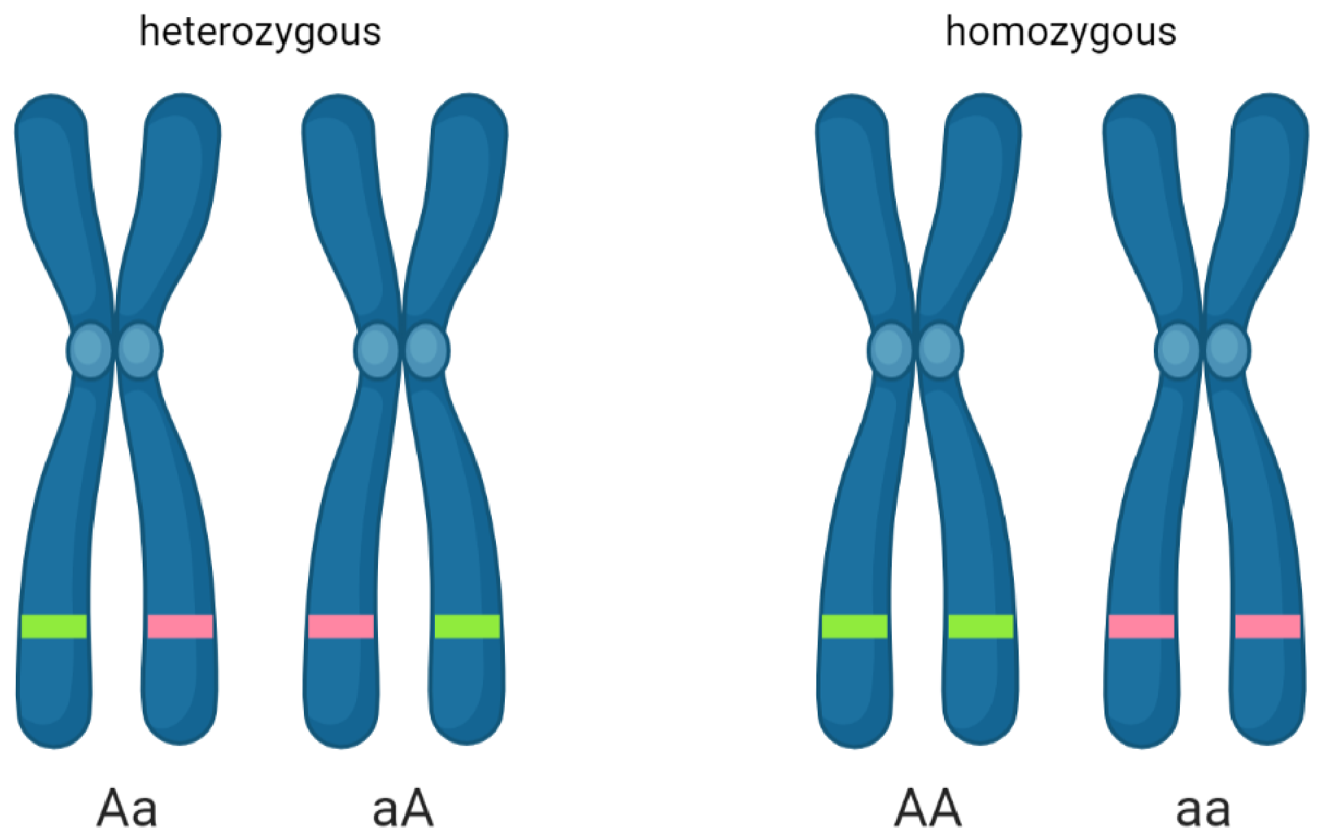
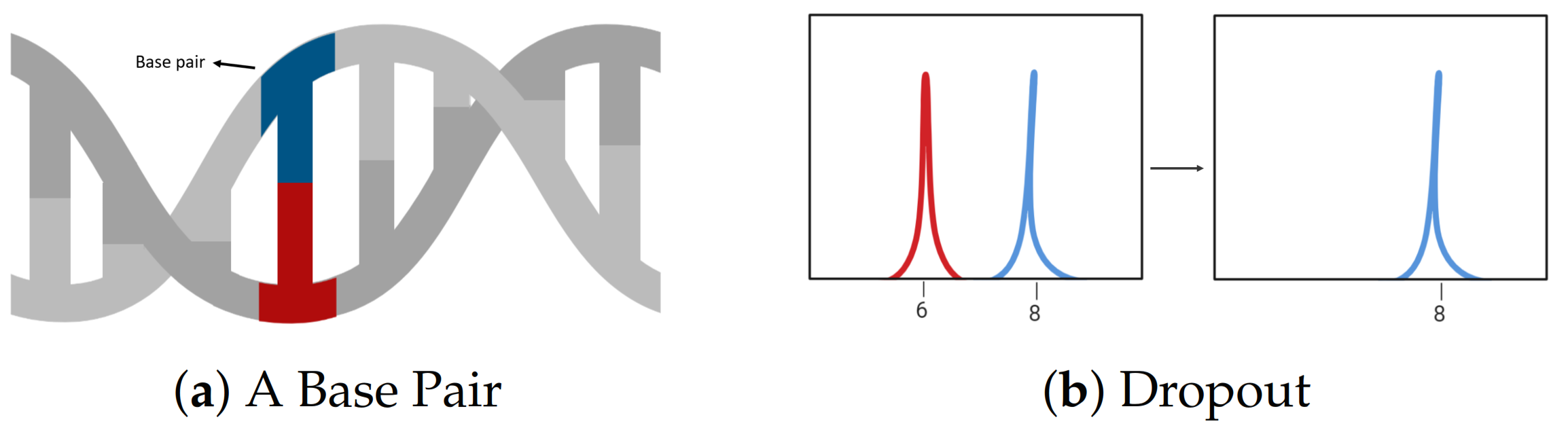
2.1. DNA Biology and Genetics

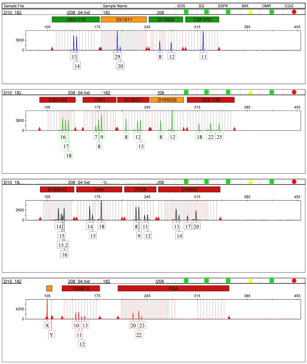
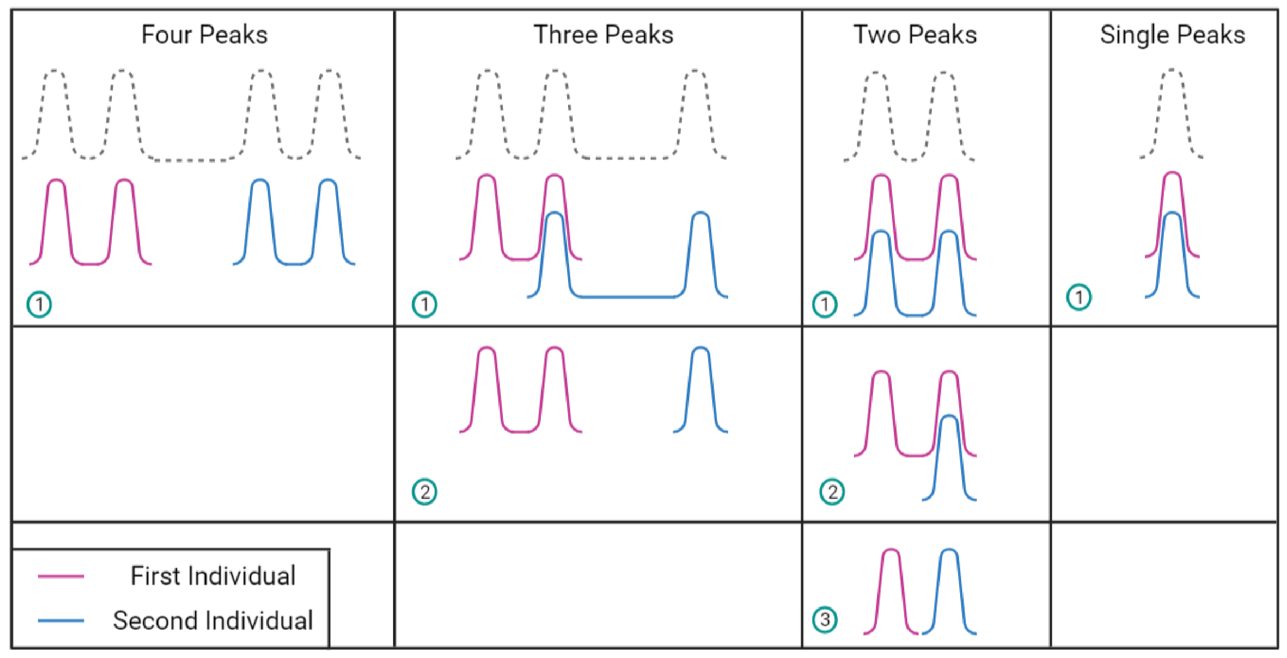
DNA is divided into chromosomes. The human cell contains 46 chromosomes (22 pairs are autosomes and one pair determines the gender). A chromosome is a structure that passes hereditary characteristics from one generation to another [1]. DNA is considered the blueprint for human physical structure. It stores all the needed information (like writing paragraphs on a book) and passes it to the next generation, with half of the information taken from the father and the other half taken from the mother. Figure 1 shows the similarity in saving information between printed text and genetic formats [1]. Human beings have many characteristics, such as weight, height, hair, and skin color. Each of these characteristics is called a trait. A marker is a specific location on a chromosome (throughout this paper, we use the terms marker and locus interchangeably) containing a gene responsible for shaping traits. Each gene has more than one form, which is called an allele. For instance, the determining gene for skin color has several alleles: an allele for white skin, an allele for brown skin, an allele for black skin, etc.

Table 1. Difference between locus, gene, and allele.

	Locus	Gene	Allele
Definition	A unique physical position on the chromosome where a gene exists.	A sequence of DNA that shapes a specific trait.	An alternate version of a specific gene.
Purpose or task	Each gene resides at one locus.	Determines traits	Responsible for transmitting the possible variations for each trait.
Number of copies	One locus in each location.	One gene in each locus.	Two (one from the mother and one from the father).
Examples	D3S1358, TH01	Weight, Height	Fat, Short

summarizes the difference between genes, alleles, and loci [1].

A chromosome is a construct that we obtain after we wrap the DNA around the nucleus. A locus refers to a specific location on a chromosome that contains a gene for some trait. A gene is a segment of the DNA that codes for a protein used to express that trait (a gene is a sequence of DNA). An allele is a pair of genes (it is an alternative form of a gene). Autosomal DNA is a part of chromosomal DNA but does not include the two sex chromosomes (X and Y). Our entire DNA sequence is called a genome. If two alleles at a specific locus are different, this case is called heterozygous, whereas if the two alleles are the same, then this case is called homozygous [1] (see Figure 2). The human being is diploid, meaning that each person has two copies of genetic instructions. If the instructions are the same (from the mother and the father), then the person is a homozygote, and if the instructions are different, the person is a heterozygote. Figure 3 and Figure 4 show an electropherogram (these are acquired from the Forensic Science Training Center (FSTC), Jeddah, Saudi Arabia, with their permission to include in our publications). It has the automated STR test results translated into a series of numbers called a DNA profile. It shows the locus names and the associated numbers, which can be quickly entered into a database. In the electropherogram, there is more than one panel; the names of the markers can be found in the boxes above the panels; the repeat numbers of alleles detected are given below the corresponding peaks. Reading an electropherogram can be carried out as follows. The D8S1179 locus has two alleles present: one is 11, and the other is 12 (their names are generated by computer software). In the mid-1990s, DNA profiles were generated, and databases appeared to store this kind of information.

Each profile has a DNA pattern related to only one person. Therefore, each location should have, at most, either two alleles or one allele (in this case, it is called homozygote). Occasionally a location will contain more than two alleles (it could be four or five, for example), and, in this case, we say that this sample contains more than one contributor; see Figure 5 (also acquired from FSTC, Saudi Arabia, with permission to publish).

The polymerase chain reaction (PCR) is a procedure for amplifying DNA by repeated duplications. The number of amplification cycles can range from 26 to 32 cycles. The amplification process takes place when more than one location is missed. The injection time can be defined as the time that the sample requires to pass the capillary on the camera that determines the locations (it can be 5 s, 15 s, or 25 s). If the alleles’ height is very significant, there could be more than one contributor in this sample.

2.2. DNA Mixtures

When a DNA profile contains more than one contributor, then this sample is called a mixture. Several markers can indicate that a sample is a mixture, such as having more than two alleles in one locus or having an imbalance (generally between 30% to 40%) in the peak height ratio (which means that there is a significant difference between the heterozygous alleles at a specific locus) [1]. When more than one person contributes to the DNA sample, this is a DNA mixture. Dealing with a DNA mixture is not easy due to the required effort and experience to detect it. When there are more loci and genetic markers, it will be easier to detect mixtures, but there are some cases where mixtures will not be detected easily, even with many loci. One of the essential factors in determining the number of contributors is the quantity of each component in the mixture sample. If each person contributes the same amount of genetic material, it will be much easier than if one person contributes a major amount and another person contributes a minor amount [1]. There are three signs that, if they occur, would indicate that this is a mixture sample, which is signified by more than two peaks for a specific locus (see Figure 6), if there were an imbalance peak height between the heterozygous alleles at a specific locus, and if there were an abnormally high stutter product.

If a DNA mixture sample came from two persons, there would be different possible genotypes based on the number of alleles that appear on the electropherogram (see Figure 7). The possible genotypes are the following [1]: having four peaks (two heterozygotes and no overlapping alleles); having three peaks (either two heterozygotes with one overlapping allele or one heterozygote and one homozygote and no overlapping alleles); having two peaks (either two heterozygotes with two overlapping alleles or one heterozygote and one homozygote with one overlapping allele, or two homozygotes with no overlapping alleles); and having only one peak (two homozygotes with an overlapping allele). Currently, the tools used for interpreting the number of contributors in a mixed DNA sample helped the analysts to determine the results. The analysts are still an essential part of this process [1].

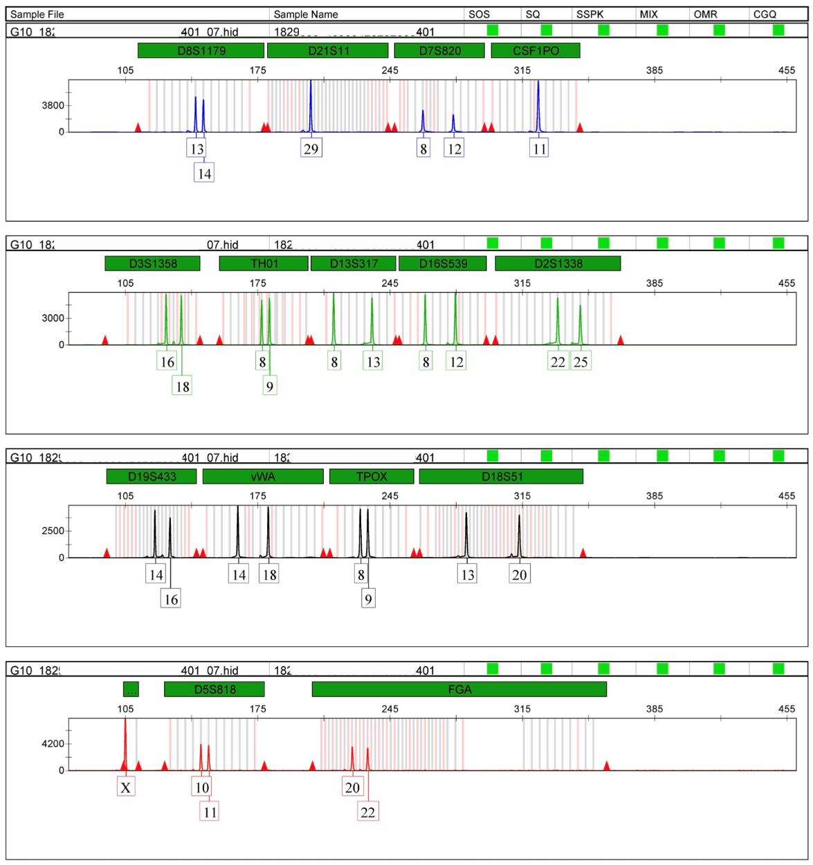
2.3. Genetic Markers

As an example of how each marker obtains its name, we will examine (D16S539). The “D” stands for the DNA, “16” is the chromosome number, the “S” indicates that this marker is a single copy sequence, and the number “539” represents the order in which the marker was discovered for this specific chromosome [1]. The DNA is divided into coding and non-coding areas. The coding region has the needed information that the cell needs to produce protein. The markers used for identity testing are located in the non-coding areas, which are called the locus (the plural for it is loci) [1].

Having more DNA markers increases confidence when comparing an evidence sample that has been taken from the crime scene and the suspect. Strong confirmation for the assessment of the analysis, showing that the two profiles are from the same source, will be achieved if the first, second, and third markers are the same. Currently, short tandem repeats (STRs) of DNA markers dominate the forensic science domain because of their ability to cope with low, degraded DNA profiles, and because they are a part of the DNA databases that are currently expanding around the world [1]. Short tandem repeats, used in genotyping, are a universal language that all laboratories around the world can deal with. They are the result of transforming the peak information that appears in the electropherogram in both DNA size base pair (see Figure 8) and quantity [1]. The height of a peak is proportional to the amount of DNA that gave rise to that particular peak during PCR amplification.

The STR markers provide a random match probability of approximately 1 in 100 trillion (assuming unrelated persons). The random match probability (RMP) can be defined as “the chance of a specific profile occurring in a specific population based on observed allele frequencies for that population" [1]. Currently, only a small amount of DNA information has been utilized, and there is still much more information that could be used. In order to calculate an estimate of the random match probability, statistical calculations will be applied to provide the estimated frequency at which a particular STR profile would be expected to occur in a population [1]. It gives a statistical weight for a DNA profile match and quantifies the chance that a randomly chosen unrelated person from a given population has the same DNA profile observed both in the suspect and an evidence sample. The amelogenin locus is a gene that resides on both the X chromosome and the Y chromosome. The X chromosome version is a little smaller than the Y chromosome version. If there is a DNA profile that has two peaks (X and Y), this is a male’s DNA profile, but if the DNA profile has two X peaks, then this is a female’s DNA profile.

2.4. Challenges in Analysing DNA Profiles

Allelic dropout can happen during the process of amplifying a low amount of DNA sample. This failure in finding an allele can occur because of some stochastic effects. Any contamination can cause allele drop-in [1]. Figure 8 shows an example of allele dropout. There is a high probability that the generated data in the electropherogram will contain noise. As a result of that, some thresholds are used to eliminate the destructive effects of the noise. In this section, we will demonstrate the two most often used standard thresholds. These are the analytical threshold, which is a standard relative fluorescence units (RFU) level (usually equal to 50 RFUs) that is considered to be suitable for use in both the PCR and STR DNA (the genetic material of an organism) typing process, where only the peaks above this value will be considered and computed, and the stochastic (or interpretation) threshold (usually equal to 150 RFUs, 200 RFUs, 500 RFUs, or 600 RFUs), which deals with stochastic effects, such as allele dropout, allele drop-in, or imbalanced allele, that occur in low-level DNA profiles. Peaks above this threshold are not affected by the previous effects. In some laboratories, both the analytical threshold and the stochastic threshold have the same values (see [1], Figure 10.2, Page 4). Any non-allelic product is considered an artifact, such as the dye blobs, which are larger than the true STR alleles [1]. There are many challenges that a forensic laboratory needs to deal with, such as having degraded DNA profiles or DNA mixtures. (See [1], Figure 14.2, Page 4, which shows the difference between a good quality sample and a degraded DNA sample [1].)

The interpretation procedure could have some artifacts, such as allele dropout, that occur when some alleles of the source cannot be caught. One way to overcome these artifacts is to gather more complex experimental data [16]. One of the ways to improve the low-level DNA profile quality is to increase the number of PCR cycles, such as from 28 cycles to 34 cycles, which will produce more DNA copies. (See [1], Figure 14.6, Page 18, which shows how increasing the number of cycles can play a key role in the allele’s imbalance and allele dropout challenges [1].) The polymerase chain reaction (PCR) is a process that is used to produce many copies from a specific desired DNA sequence through repeated cycling of reactions. Any failure in making multiple copies could affect the chance of properly analyzing DNA profiles, especially the low and degraded (broken into mini sections) DNA samples. The common number of iterations is 28 cycles, 32 cycles, or 34 cycles [1]. It is the primary method that molecular biologists can use to amplify DNA in their laboratories (not the whole DNA but a specific region of DNA that they can choose). Empty sections of the graph mean that there could be an error in the sample. The solutions here are to leave it empty or increase the number of cycles (for example, if 27 cycles were used, now, 29 cycles will be used).

2.5. Forensic Science and DNA Profiling

Lynda Mann and Dawn Ashworth were two young girls who were murdered in different time periods in a single village in England. Due to the fact that the two murders occurred in similar circumstances, the police started to think that both of these crimes were carried out by the same killer. They suspected a man, but then they found that his DNA did not match the DNA that had been taken from the crime scene. They also took a sample from 4000 other men, but there was no match. After two years, a woman noticed a man who was proud of giving his blood sample to his friend, Colin Pitchfork. The police then took a sample from him and, as they suspected, his sample matched the profiles from the crime scene. After that, he was sent to prison for life. This is the story behind the first use of DNA typing in the forensic science domain [1].

DNA profiling, typing, or fingerprinting are three terms for the same concept. It is a method that was proposed by Jeffreys in 1985. This process attempts to identify a person based on his or her DNA sequence and its differences from the DNA of other people. This method has been considered a revolution in the forensic science domain, since the development of the fingerprinting process. The method plays a crucial role in many applications, such as parentage testing, disaster victim identification, and missing person investigation. However, there is a misunderstanding about the amount of time needed and the amount of effort to obtain the results [1]. The idea behind DNA typing is suggested because, in any DNA sequence, there are specific patterns that are repeated and are adjacent to each other. This is a variable number of tandem repeats, VNTRs, which, if within a range between 8 and 100 base pairs, and with a length of between two to seven bases, are called short tandem repeats, STRs. Another interesting finding is that the number of repeated patterns differs between individuals (called length polymorphism). From this point, a technique called restriction fragment length polymorphism (RFLP) was developed [1]. The goal of this procedure is to extract these VNTRs repeats from the DNA sequence. The markers on the autosomal chromosomes are used to perform identity testing (see Figure 9) [1].

If a sample has two alleles (12,17), this means that the first allele comes from the father, for example, and was repeated 12 times. The second allele comes from the mother, for example, and was repeated 17 times [1]. Genotyping (DNA profile) is achieved by comparing the allelic ladder (the bins that the software manufacturer has previously defined) and the given sample. Each peak found inside a particular bin will be considered and adopted as an allele for this specific locus ([1], Figure 10.4, Page 6). In some cases, the analyst’s decision is needed to determine if this peak is a true allele or an artifact [1]. There are some situations where the given sample contains peaks that do not fall inside any allele’s bins. These peaks are called off-ladder or variant alleles. Three types of these situations are illustrated in [1] (Box 10.1, Page 8). A ladder is an important concept and it is necessary to understand it. This measuring rule is used for location determining and helping in giving values for both the alleles’ height and size. The abbreviation, OL, is used to indicate that this specific location does not exist in this ladder, but that it does exist at some location. The OL is a unique signature for an individual. It can be computed manually (and, here, we need the .fsa files), or the specialist can leave it empty. One example of the OL is when someone has three alleles instead of one or two.

One of the critical tasks in forensic science is determining the contributor number in the evidence sample to determine if this sample belongs to one person or more. This sample is called a mixture if there is more than one contributor in the DNA sample. It is the analysts’ job to make this decision. This will be accomplished by examining the number of alleles at each locus (whether there are more than two peaks at a locus), the strictly imbalanced peak height, and other artifacts, such as stutter (which is an additional peak that is shorter than the real peak), air bubbles, sample contaminants, and dye blobs (see [1], Figure 10.5, Page 13) [1]. In USA, more than 300,000 paternity tests are performed annually. This test requires three profiles to give the results: one each from the child, the mother, and the suspected father. This test is used to see if there is a shared allele between the suspected father and the child [1]; see

Table 2. Non-direct comparison (paternity test).

	Wife	Son	Potential (Father)	Actual Profile
D5S818	11, 13	11, 13	11, ? or ?, 13	12, 13
D13S317	8, 12	8, 14	?, 14	11, 14
D7S820	8, 12	8, 9	9, ?	9, 9
D16S539	8, 9	9, 13	?, 13	11, 13
CSF1PO	10, 12	10, 10	?, 10	10, 10
Penta D	8, 10	9, 10	9, ?	9, 12

.

DNA polymorphism (many forms)is a region of DNA that is very likely to differ from one person to another simply because, as its name implies, it comes in many different forms. Electrophoresis is the method used to separate DNA molecules based on their size (big molecules require more time to move than small molecules). When there is DNA testing, the objective is to obtain DNA from a reference sample, such as blood, and to compare it to the genetic material that has been collected from an evidence sample. The first step in this process is quite simple. It is to extract and purify DNA from both materials. The purification steps are not very complicated.

Coquoz [16] provides fundamental information related to both forensic science and bioinformatics fields. DNA is considered an essential tool that links biological evidence and suspects. For any pair of persons, the DNA sequence is almost the same. However, many slight differences provide the ability to distinguish between these two persons. This inter-individual variability is also called polymorphisms. When a polymorphism is used in forensic science for identification purposes, it is called a marker, and the variants at the polymorphic positions are called alleles. The difference can be slight at the single-nucleotide level, and, in this case, it is called a single nucleotide polymorphism (SNP). The difference could also come from repetitive nucleotide sequences where it is “repeated in tandem like a series of identical beads on a necklace”. A polymorphism is the difference in the number of repeats. Alleles will have different sizes so that their names will be based on the number of repeats they have. For example, if the repeat unit is larger than six nucleotides, the repeat unit is called a minisatellite or VNTR, and when it is less, it is called a microsatellite or STR. From 1968 to 1995, DNA profiling used VNTRs as a marker. Currently, the focus has moved to STR and SNP markers. The polymerase chain reaction (PCR) is a technique used to create DNA amplification by repeatedly stimulating the natural DNA duplication process. It can be considered a loop, and, at the end of each iteration, the number of copies of a specific sequence will be doubled. Analyzing a set of STRs will produce a DNA profile. Two DNA profiles would be comparable only if there are a few STRs in common.

2.6. Likelihood Estimation

Likelihood ratio estimation (LR) is one of the methods for the estimation of the number of unknowns in a DNA mixture. It is a popular method for estimating the number of unknowns in DNA mixtures and, hence, we discuss it here. The likelihood ratio is the ratio of two probabilities of the same event under different hypotheses. The defense hypothesis is abbreviate Hd, and it is the denominator in a likelihood ratio, whereas Hp is the prosecution’s hypothesis, and is the numerator in the likelihood ratio. The likelihood ratios and combined probabilities of inclusion/exclusion are used for the statistical evaluation of mixed DNA profiles [1]. The interpretation procedure depends on the Bayesian evaluation by having two hypotheses: the hypothesis of accusation (the mark comes from the suspect), or the hypothesis of defense (the mark comes from another person). Any DNA evidence should be evaluated by comparing these two hypotheses. The evidence interpretation is stated as a ratio of the probability that the evidential material has the same source as the comparison sample (the hypothesis favored by the accusation) to the probability for the evidence that someone else is the source of the evidence (the hypothesis favored by the defense). The likelihood ratio forms some of the core elements of the Bayesian framework of evidence interpretation. When the ratio is greater than one, it supports the accusation, and when it is lower than one, it supports the defense hypothesis.

Alfonse et al. [14], in introducing their PROVEDIt dataset, point out that the likelihood ratio (LR) framework is the statistical comparison of unknown profiles to profiles taken from known persons. This approach compares the probability of the data assuming two hypotheses: either the person of interest (POI) contributed to the profile or did not contribute. The LR approach replaced the traditional methods involving manual interpretation and jumped toward utilizing probabilistic models to evaluate unknown profiles. This was carried out primarily because of the complex nature of low template and multi-contributor DNA samples that prompt the need for the continued research and development field of human identification. The authors state that the current challenge in this area is developing methods and tools that exploit all information contained within the data.

2.7. DNA Databases

As a result of the significant benefit and the great impact that every DNA sample could provide to society, the criminal justice system, and the forensic science domain in recent years, DNA databases have begun to appear. One such database is the National DNA Index System (NDIS) database, which includes more than 6.5 million STR profiles that help when searching for any suspect’s DNA profile, connecting them to serial crimes, and providing critical evidence. A DNA database is a repository for all the digital STR genotypes (DNA profiles) that allows one to search through it to find a potential match to any given sample. The number of used STR markers is different between some countries, and, because of that, some data are not compatible between these countries and their different laboratories. In order to have a DNA database, there are four essential components that must be present: having many DNA profiles that are necessary to feed the database; a standard set of DNA markers that will help in the comparison process; reliable software and a secure network, especially when sending and receiving profiles from various laboratories; and quality assurance standards that will decide if the results are trustworthy or not because having an inaccurate DNA sample will create harmful effects in the entire database.

Having a national DNA database is not a new trend. The first national DNA database was established in 1995 in the United Kingdom. It now contains more than four million DNA profiles. This encourages other countries, such as Canada, New Zealand, Australia, and Japan, to have their own DNA databases. Most of the countries use the same STR markers. Having access to DNA databases is fundamental in providing researchers with the ability to test their hypotheses. Unfortunately, privacy concerns mean that this is not an easy task. However, a small number of DNA databases are accessible online, and they overcome the privacy issues by providing the DNA profiles with no names of the associated persons, so there is no chance to link the DNA sample with a known person. Nevertheless, these online databases have their challenges, such as the quality, which is not high (it could contain a lot of missing information) [1]. The idea behind having a small population dataset is to estimate random match probabilities based on an allele frequency measurement from a group of persons selected to represent a specific group of interest. Due to the fact that it is impossible to gather all of the DNA profiles from all of the humans on the planet, random match probability (RMP) and likelihood ratios (LR) are two ways to calculate the rarity for a particular DNA profile. This estimation depends on three factors: the DNA profile’s alleles, the population allele frequencies that have been used, and the genetic formulas that compute the degree of relatedness (see Figure 10). The result of this estimation is the frequency for the given DNA profile in a population. The population datasets aim to evaluate how common or rare a specific allele or alleles sequences are. The one extensive database of forensic use in the United States is the Combined Offender DNA Index System (CODIS) database. The Federal Bureau of Investigation maintains this database. This database can be used as a potent investigative tool by law enforcement officers.

3. Related Works

This section reviews notable works related to this paper. We purposely discuss these methods in detail to provide this paper as a source for a background and literature review on DNA profiling. We divide DNA profiling methods into three categories and will discuss them separately. Section 3.1 discusses the basic methods in determining the number of contributors. Section 3.2 discusses the parallel methods used, and Section 3.3 reviews the methods that use machine learning. Section 3.4 reviews machine-learning-based works in the broader area of bioinformatics.

3.1. Basic Methods and Tools

Several methods exist that can be classified as the basic methods. Examples include the maximum allele count method (MAC) [3]. It divides the largest number of alleles by two and rounds it up to the nearest whole number. Although this method is trivial, mischaracterization could occur when the mixture is complicated because of having more than two contributors, allele sharing, and degraded or low-template DNA. Another method is the total allele count (TAC), which uses the total number of alleles and peak heights (PH), MLE [4], and NOCIt [7], and requires a very long processing time when dealing with a large number of unknowns (for example, a five-person mixture takes up to nine hours to evaluate). Other notable tools in this category include DNA mixtures [17], Lab Retriever [18], and DNAMIX [9]. A review of the methods and tools for DNA profiling has been reviewed in [2], focusing on computing the number of unknown contributors in a DNA mixture.

3.2. HPC Methods and Tools

The progress on methods and software for solving the DNA mixture problem had stagnated due to the exponential computational complexity of computing the number of unknowns in a DNA mixture [2,11]. Although there is some work based on the use of a software package called OpenMP on shared memory machines to deal with this challenge, they were applied to small problems only. The work that developed parallel implementations on single nodes included Euroformix [9], LikeLTD [10], and (NOCIt) [7]. Alamoudi et al. [2,11] developed multiple parallel implementations of DNA profiling, focusing on the maximum likelihood computations. The first implementation was based on OpenMP on shared memory nodes and it achieved a 3x speed up compared to the NOCIt tool. However, the shared memory could not deal with a number of unknowns larger than five and, hence, they developed a hybrid OpenMP/MPI implementation for distributed memory architectures. This is reported to be the first ever hybrid distributed memory implementation of DNA profiling, enabling the likelihood ratio computations to scale to virtually any number of unknowns. Using this implementation, the authors reported results for up to ten unknowns, delivering over 15× the performance of OpenMP using up to 3072 cores. None of the earlier works had reported dealing with mixtures containing this number of unknowns.

3.3. Machine Learning in DNA Profiling

Artificial intelligence (AI), including machine and deep learning, has been increasingly applied to replace human intelligence and other mathematical algorithms in many fields, such as IT operations and management [19], healthcare [20,21], transportation [22,23,24], education [25], smart cities [26,27], accident and disaster management [28], big data [29], improving computing algorithmic [30,31], spam detection [32], and gender classification [33]. We have mentioned earlier that there are only four ML-based methods for the estimation of contributors in DNA mixtures. We discuss these in chronological order.

Marciano and Adelman [12] aimed to apply machine learning algorithms in the bioinformatics field by estimate the number of contributors in a DNA mixture. The study highlights the need to know the number of contributors to deconvolute a DNA mixture, although other metrics are also necessary to effectively deconvolute DNA mixtures, such as the contributor ratio and allele drop-in and dropout probabilities. Several kinds of research substantiate the belief that there is a need for discovering the number of contributors. For that reason, there are several methods proposed to deal with this challenge. This study goes through some of these methods and demonstrates both the strengths and weaknesses for each one of them. In recent years, much attention has been drawn to machine learning. The model is trained with an existing set of data, after which, what it has learned will be generalized. This means that even if there are new data passed to the model, it will have the capability to deal with those data. Machine learning is applied in many applications, such as in natural language processing, object-oriented, and DNA sequence classification. However, little research has been conducted to study the application of machine learning in estimating the number of contributors precisely.

In the authors’ opinion [12], this kind of problem could be solved by applying machine learning, because, in this challenge, there is a vast repository of human DNA mixtures, which comprises a high-dimensional and complex data set in an electronic format. Machine learning has shown, in many studies, that it can deal with this kind of challenge. For that reason, the authors in this article propose an approach for determining the number of contributors in a DNA mixture using machine learning algorithms. The authors assess six machine learning algorithms’ classification performances and evaluate them. The algorithms are the K-nearest neighbors algorithm, classification and regression tree, multinomial logistic regression, multilayer logistic regression, multilayer perceptron, and support vector machine. The system was trained, tested, and validated using electronic data (.fsa files). It was taken from 1405 non-simulated DNA mixture profiles comprising one to four contributors, and it was generated from a combination of 20 persons with different DNA template amounts and different ratios of contributors. The profiles were amplified using the AmpFLSTR Identifiler PCR amplification kit (28 cycles) (15 STR loci per profile). In order to pass new data when testing the system, the dataset was portioned into a training dataset and a testing dataset. For the feature scaling phase, the features that were considered were the peak height, allele count per locus, etc. For the feature selection phase, the Kullback–Leibler divergence was used. All candidate features are ranked by divergence, and any candidate feature less than 0.01 is removed before the machine learning phase. The results show a 98% accuracy in the training stage and 97% accuracy in the testing stage in identifying the number of contributors in a DNA mixture of up to four contributors.

Benschop et al. [13] propose a machine learning model that computes the number of contributors (NOC) using a random forest classifier with 19 features, and, because of that, they call the model (RFC19). They compare their results with the MAC and nC-tool (based on TAC) and report a better accuracy. The authors emphasize that determining the number of contributors in an STR (short tandem repeat) is a complicated task due to many factors, such as allele dropout and allele sharing. They claim that the accuracy could be improved by increasing the numbers of markers and taking benefits from other information rather than depending only on the allele counts. The authors created their own DNA mixture profiles dataset for this study. They use 590 PowerPlex Fusion 6c Profiles (PPF6C). The DNA data were collected from 1174 different donors and created various DNA mixture profiles containing one to five DNA contributors. The resulting profiles were different in terms of allele sharing levels, allele dropout, mixture proportion, and amount of DNA. The dataset was then divided into three sets (training, test, and holdout). There were more than 250 characteristic features that depended on the allele count, frequencies, and peak heights for each profile.

The authors clarify that, currently, there are many advanced probabilistic genotyping software applications that deal with complex DNA profiles. However, most of this software needs to know the contributor numbers in advance. For that reason, several contributions emerged, such as the maximum allele count method (MAC) and total allele count (TAC), which use the total number of alleles and peak heights (PH). The authors state that the distribution of allele counts over the loci, allelic dropout, and stutter probabilities, or Bayesian network approach, should improve the estimation of the number of contributors. The key is to exploit the presented profile information by using a machine learning approach that can estimate the number of contributors in seconds, and that deals with this challenge as a classification problem, where the classes are the contributors’ numbers. The main goal for classification is to identify the category or class into which new data will fall. The authors state that developing the model happens in two stages. First, the informative DNA profile characteristics features for the number of contributors are chosen (278 features per profile). Then, the machine learning classifiers are selected. A model is developed by combining both features and the algorithm. The training data (which contain each DNA profile, its features, and the identified number of contributors) should provide the required environment for the algorithm to gain experience regarding the features that best fit a single contributor, two contributors, etc. The performance for the training model was calculated by testing it with another dataset whose labels are not known to the model.

By that time, there was only one machine learning model, PACE software, that infers the number of contributors in autosomal DNA profiles. This software is based on a support vector machine classifier, and it outperformed the MAC method. The dataset was a form of one to four contributors. To ensure that the dataset represents forensic casework, the authors gave the DNA profiles to a qualified reporting officer who performs forensic casework daily. There were two other datasets in addition to this dataset. One set is created to represent the extremely complex DNA profiles (such as having a mixture generated from related persons with dropout, having a degraded DNA mixture with a minimum of three locus dropouts, or having six persons in a DNA mixture). The purpose of these sets is to observe the limitations of the RFC19 model. The other set was created to examine the effect of the replication on the model. The authors next train and test ten classification algorithms 50 times, and compute both the precision and recall for each model in order to choose the most promising ones from them. The best model was validated through the holdout dataset. Both datasets were applied to examine the model’s limitations and effects. The results of the model were compared to the results of both the MAC method and nC-tool. The nC-tool is an Excel spreadsheet that uses some correct TAC of a particular DNA profile and compares it with the obtained TAC. The output is a probability for each number of contributors.

The authors use partial correlation to select the features because, if a large number of features are chosen, this could lead to overfitting. If a small number of features are chosen, vital information may be ignored. Fifty features resulted from the partial correlation, and they were used in both training and testing phases. Two models showed promising results: random forest classifier, with 19 features (RFC19), and linear discriminant analysis, with 40 features (LDA40). The authors compared RFC19 and LDA40 and found that, although LDA is a simple algorithm, it requires double the number of features compared to RFC. Hence, RFC19 was selected. The authors examined three datasets on the RFC19 model. The first was a mixture of six persons. The second was a generated low mixture of relative persons, and the third was a degraded mixture. The model in these three cases gives an incorrect prediction. However, the authors believe that this mischaracterization is because the RFC19 is not trained on these datasets. In addition, the authors performed a replicate analysis on the RFC19 model, and they found that the precision for the joint replicates was higher than the person replicate. The results show an 83% accuracy. In the end, the authors summarize their future work on six points. First, both the amelogenin and Y-chromosomal markers were excluded from the analysis, but they could be used in the future. Second, the datasets can be extended by combining a female’s DNA profiles. Third, increasing the number of features characteristics. Fourth, as mentioned previously, applying replicates improved the accuracy of the RFC19 model. In the future, the model should be trained on a dataset that has been replicated. Fifth, examining possible enhancements in performance when swapping from classification algorithms to regression algorithms, and, finally, to help the end-user understand the model’s results, presenting feature importance.

Kruijver et al. [15] propose a semi-simple method that uses decision trees. What makes this method different is that it runs quickly, and the forensic expert can understand why they obtained these specific results. In order to accomplish their work, the authors used part of the PROVEDIt dataset. The authors show that the performance of the filters used has a significant impact on the method’s performance. Determining the NOC is a time-consuming process, and the results may differ between one analyst and another based on their experience with the procedure. In their work, the authors mention three challenges that make the interpretation process a complicated task. The first one was having more than one allele shared between different contributors. The second one is having a dropout allele, or having an allele below the analytical threshold. The last one is when stutter peaks (or alleles) exist. The authors mention that most of the contributions currently use statistical classification methods that depend on MAC, TAC, and the number of loci with three to four alleles. By performing those, these contributions helped the classification process to be performed in a faster manner. However, to have accurate results, a large dataset is needed to train the model on, and it will be hard for the forensic analyst to understand how the model obtained these particular results. In their work, the authors combined the MAC method with an assessment of the peak heights. They also emphasized that no one statistical method can be considered dominant for this challenge.

The authors also mention that the current contributions are different in terms of the multiplexes used, the profiles types, and the different metrics used to evaluate the performance. One of the interesting points that they mention is that it is helpful to know how many persons contributed to a sample. This is because, for example, when adding more than one contributor to a sample, occasionally one or more alleles can be shared or below the analytical threshold (AT), and, as a result, the profile will appear to have a smaller number of contributors. In order to measure how accurate the model is, the authors mention two methods. First, by comparing the obtained results with the analyst assigned values (this way, it is subjective) or, second, by comparing values that have been taken from another tool.

The authors mention that one of the essential factors in determining the NOC is the pre-processing data stage, including filtering both stutter and other artifacts. For example, if one stutter remains, this will possibly lead to having inaccurate results. The authors use decision trees to determine the persons in a DNA mixture. A decision tree is a map (this consists of if/then questions) of the possible outcomes (in our case, the NOC) of a series of related choices. For example, the number of alleles in the profile, allele heights, and the minimum (and maximum) number of alleles at a specific locus. They use decision trees because it is a straightforward method and easy to understand. The authors used three different stutter and artifact filtering methods to compare the performance of the proposed decision trees. They compare their work with NOCIt, MAC, and RFC19 models. The data that they worked on were taken from the PROVEDIt dataset. It consisted of 100 profiles that contained only one person, whereas 666 profiles contained two to five contributors, amplified with GlobalFiler multiplex—3500 genetic analyzers with 25 injection times. The training set consists of 300 profiles that were chosen randomly. The remaining 466 profiles were used to compare the accuracy between the proposed method and the previous contributions. The data were split into six different training datasets (100, 200, 300, 400, 500, and 600 profiles), and the testing profiles were those remaining for the proposed method. It is worth mentioning that the training sets were generated 1000 times. The authors state that, when implementing a decision tree, it is better to use more profiles; however, this provides additional costs. They also found that the performance is better when the injection time is 25 s because more alleles appear. They also mentioned that ML approaches have been demonstrated to achieve a better predictive performance than a decision tree approach. They also said that this ML approach required some time to train. Furthermore, they emphasized that the accuracy decreases for higher-order mixtures. In conclusion, the decision tree method has been shown to have an accuracy of 77.9–85.2%.

Finally, the last work is our own work [6], where we investigated the performance of six machine learning algorithms for estimating the number of unknowns on a small subset (780 profiles) of the PROVEDIt dataset. The difference between this work and the work presented in this paper is that the previous work used machine learning algorithms as opposed to deep learning in this paper. More importantly, we did not investigate the ML performance in detail, such as in this work, by developing various subsets of the dataset exploring performance against various multiplexes, loci, and profiles.

3.4. Machine Learning in Bioinformatics

To augment the literature on machine learning for DNA profiling, in this section, we provide a review of machine-learning-based works in bioinformatics. This is expected to be useful for the reader to understand the current developments in machine-learning-based methods for the problems in the broader area of bioinformatics. Hung and Tang [34] review deep learning tools and frameworks for bioinformatics. They limit this review to GPU-based tools alone. The authors also survey relevant deep learning algorithms. This study arises because recent studies have asserted that deep learning algorithms show a higher performance (in terms of their prediction and classification accuracy) when compared to the traditional analytic methods when dealing with biological data that are increasing quickly, especially in pattern recognition in the bioinformatics field. Both convolution neural networks (CNN) and recurrent neural networks (RNN) were used in gene expression analysis, enhancer and regularity region prediction, and methylation prediction. Most of the frameworks are easy to obtain (some of them already have a graphical user interface instead of the command line mode). Various frameworks benefit from the GPU computing power, such as Caffe, which is used to implement CNNs for image recognition and supports distributed learning on a cluster system. However, it does not support RNN or CNTK, which is used to implement CNN and RNN models to train on different kinds of data. TensorFlow supports models performed on CPUs, GPUs, and the multiple compute nodes on a cluster. Theano is used to implement mathematical expressions on CPUs and GPUs. Torch supports the implementation of CNN; however, it is not suitable for RNN. Finally, MXNET has the availability to scale up the computational performance on multiple machines and GPUs. The authors strongly believe that computing power plays a serious part in deep learning, so many hardware architectures have been developed to enhance the computational performance. For that reason, a high performance was suggested in the article to speed up the training process.

Larranaga et al. [35] review machine learning methods in the bioinformatics field. Much attention has been drawn to the biological data that have recently grown in an exponential manner. With this growth, many challenges appear, such as needing efficient information storage and management, and a valuable tool to extract knowledge from these data. Machine learning is commonly used in biological domains to extract knowledge from data, such as genomics, proteomics, microarray, system biology, evaluation, and text mining. Prior research generally confirms that complex experimental data raise two main problems: the need to preprocess the data, and the required analysis to extract the desired information.

Olson et al. [36] surveyed 13 machine learning algorithms applied to 165 classification problems in biology and medicine. This survey appeared because of the rapid growth in the bioinformatics field, and this growth was due to a demand to have both new data and new algorithms. Several studies agree that machine learning is becoming a key role in bioinformatics when conducting predictive analytics and better understanding the complex biological process of the human body. These studies have proven that there is a substantial interest in machine learning algorithms for bioinformatics applications. Although there are numerous readily available machine learning algorithms, several researchers have fallen into choice overload and struggle to select the suitable machine learning algorithm for their problem. The authors stated that choosing a suitable machine learning algorithm will improve the accuracy problem of the predictions, so this choice is a critical decision. The authors compared 13 popular machine learning algorithms, and, for each algorithm, the hyperparameters were tuned using a fixed grid search with ten-fold cross-validation. The algorithms were compared on 165 supervised classification datasets from the Penn Machine Learning Benchmark. For their conclusion, the authors recommended five algorithms with hyperparameters based on their significant performance across tested problems as a starting point for further researchers. These are the gradient boosting classifier, random forest classifier, SVC, extra trees classifier, and logistic regression. For future work, the authors intend to give more attention to regression used in several biomedical applications, improving the model performance by considering feature preprocessing, and analyzing the dataset properties that influence the performance of specific algorithms. The authors believe that it is possible to generate recommendations about the best machine learning algorithms that work well for specific applications.

4. Methodology and Design

This section discusses the methodology and the design of our proposed work. Section 4.1 provides a brief overview of the PROVEDIt dataset, its content, and the three scenarios used with the TAWSEEM model. Section 4.2 presents the pre-processing stage. The TAWSEEM model is proposed in Section 4.3, and the evaluation metrics will be shown in Section 4.4. Figure 11 provides a high-level view of the TAWSEEM tool.

4.1. PROVEDIt Dataset

Alfonse et al. [14] provide a dataset that contains over 25,000 multiplex STR profiles formed from one to five known persons, ranging from simple to complex profiles. They called it PROVEDIt (Project Research Openness for Validation with Empirical Data). They believe that such a big dataset will provide a noticeable contribution in demonstrating both the validity and robustness of new DNA methods and tools. The testing of DNA is accomplished by comparing STR regions of known STR profiles with unknown STR profiles, such as profiles that have been taken from a crime scene. These profiles usually consist of incomplete STR profiles from an unknown number of unknown contributors. The authors indicate that analyzing a forensic sample is a challenging task due to several factors, such as noise and stutter, which will lead to an STR profile consisting of missing data.

The dataset was generated over a period of more than four years using 144 different laboratory conditions. The DNA profiles range from one to five persons. The dataset comprised profiles that might be encountered in actual cases. The dataset is divided into raw, filtered, and unfiltered sections. Several interpretation tools, analysis techniques, and interpretation standards have been developed to deal with the DNA mixtures. As a result of that, this empirical dataset was produced to give the ability to compare, contrast, and validate these computational systems. The dataset consists of 26 folders; see Figure 12. The folders in the dataset can be decomposed into four sections. 1. The filtered data (one folder); 2. The unfiltered data (one folder); 3. One person profile (12 folders); and 4. Two to five-person profiles (12 folders). The GlobalFiler folder provides an example (note that the other folders have the same content). It contains two folders and one Excel file. The first folder (1-person) contains three different folders based on the injection time (5 s, 15 s, or 25 s). Each one of the three folders contains one Excel file. The second folder (2–5 person) also contains three folders, different from each other, based on their injection time. The third file is an Excel file that describes the genotype for each sample. This file contains the allele, size, and height for all peaks.

For the filtered data, Figure 13 and Figure 14 summarize the content of each multiplex. The first three multiplexes contain 16 markers, except the last multiplex (GlobalFiler (29 cycles)), which contains 24 markers. Note that in [15], the authors used 766 profiles from the PROVEDIt dataset. Among these profiles, they found a five-person mixture that was wrongly labeled as a two-person mixture. An example is given (see [15], Figure B1, Page 10). Figure 13 (on the left) visualizes the content for the Identifiler Plus multiplex when the cycle number is 28 cycles. There are five different sets of bars, which are the number of the contributors. Within each group bar, each bar represents a different injection time. For example, the number of profiles containing a two-person mixture when the injection time is 20 s is 2655. The highest number of profiles is in the one-person group when the injection time is 5 s (2810 profiles), and the least number of profiles is in the five-person group (152 profiles). Note that the numbers of profiles for 2, 3, 4, and 5 persons are almost the same. However, the one-person profiles are, significantly, the highest, and this will cause an imbalanced problem that we will discuss later.

Figure 13 (on the right) visualizes the content for the Identifiler Plus multiplex when the cycle number is 29 cycles. There are five different sets of bars, which represent the number of contributors. Within each group bar, each bar represents a different injection time. For example, the number of profiles containing a three-person mixture, when the injection time is 25 s, is 69. The highest number of profiles is in the one-person group when the injection time is 5 s (788 profiles), whereas the least number of profiles is in the four-person group (49 profiles). Note that the number of profiles for 2, 3, 4, and 5 persons are almost the same. However, the one-person profiles are, significantly, the highest, and this will cause an imbalanced problem that we will discuss later.

Figure 14 (on the left) visualizes the content for the PowerPlex multiplex when the cycle number is 32 cycles. There are five different sets of bars, which represent the number of contributors. Within each group bar, each bar represents a different injection time. For example, the number of profiles that contains four-person mixture when the injection time is 20 s is 20. The highest number of profiles is in the one-person group when the injection time is 5 s (355 profiles), and the least number of profiles is in the three-person group when the injection time is 20 s (14 profiles). Note that the number of profiles for 2, 3, 4, and 5 persons are almost the same. However, the one person profiles are, significantly, the highest, and this will cause an imbalanced problem that we will discuss later.

Figure 14 (right) visualizes the content for the GlobalFiler multiplex when the cycle number is 29 cycles. There are five different sets of bars, which represent the number of the contributors. Within each group bar, each bar represents a different injection time. For example, the number of profiles containing a five-person mixture when the injection time is 25 s is 156. The highest number of profiles is in the one-person group when the injection time is 5 s (2742 profiles), and the least number of profiles is in the five-person group (156 profiles). Note that the numbers of profiles for 2, 3, 4, and 5 persons are almost the same. However, the one-person profiles are, significantly, the highest, and this will cause an imbalanced problem that we will discuss later.

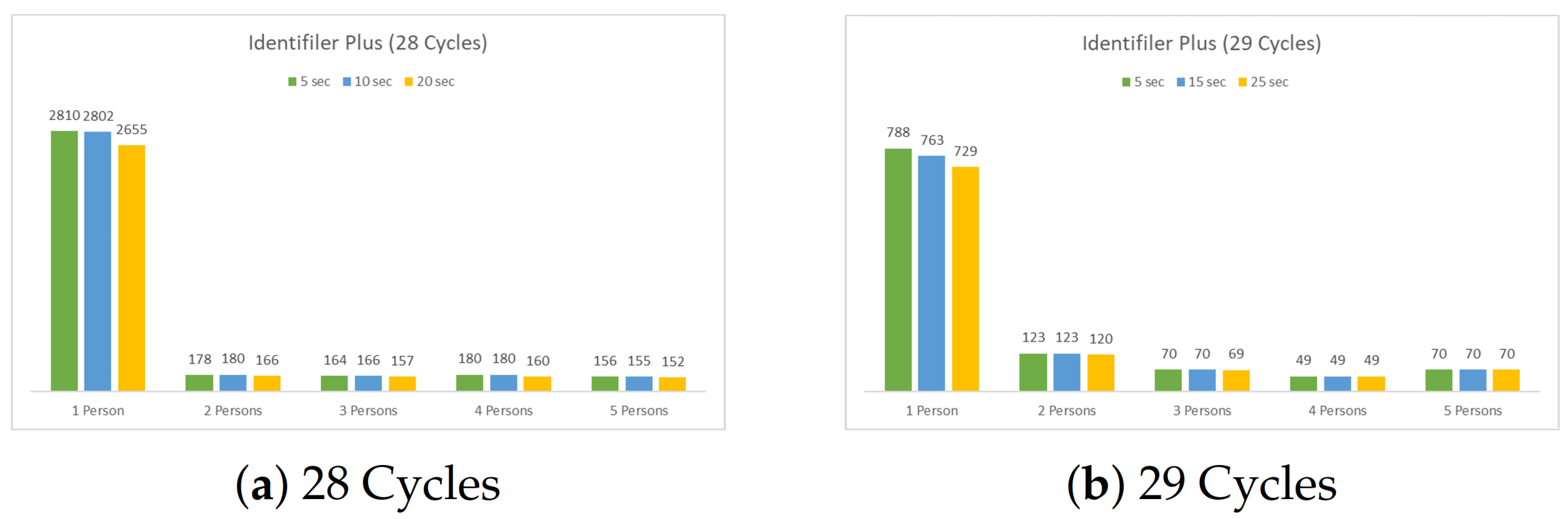
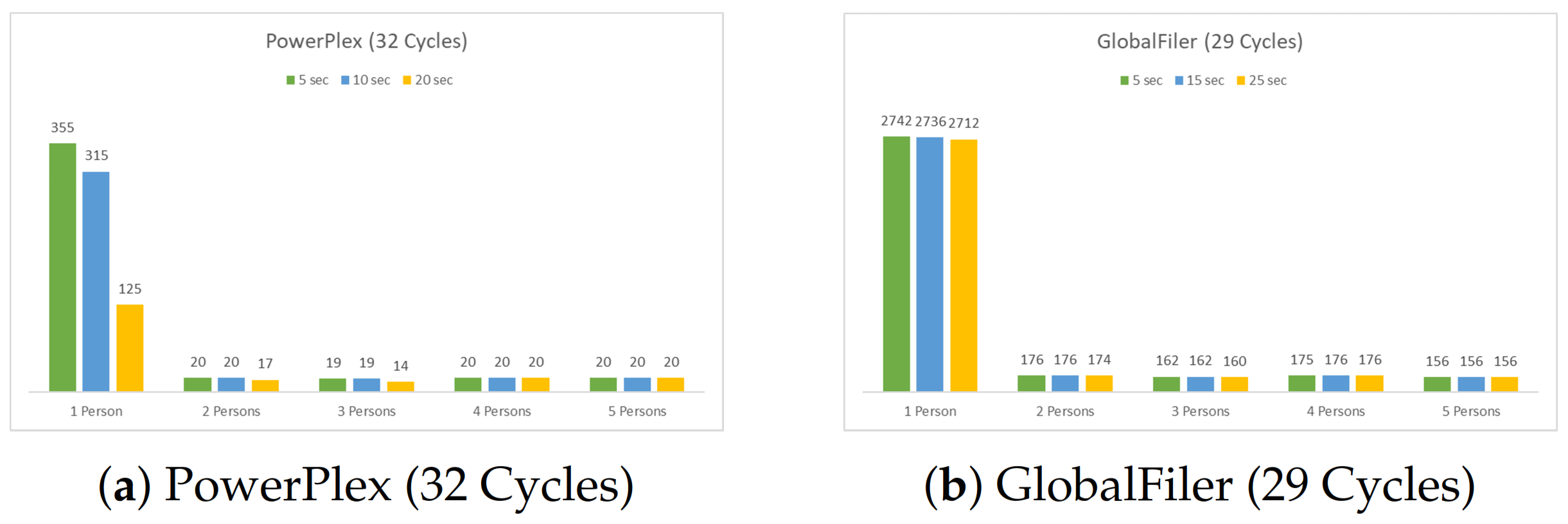
4.1.1. Single Multiplex Profiles

We chose to use the GlobalFiler (29 cycles) (see Figure 14). To work with one injection time and a balanced dataset, we chose the 25 s injection time and took 156 profiles from each class to have 780 profiles. Due to the fact that each sample has 24 markers, there will be 18,720 rows (156 × 24 × 5 = 18,720). We added the labeling column to the dataset.

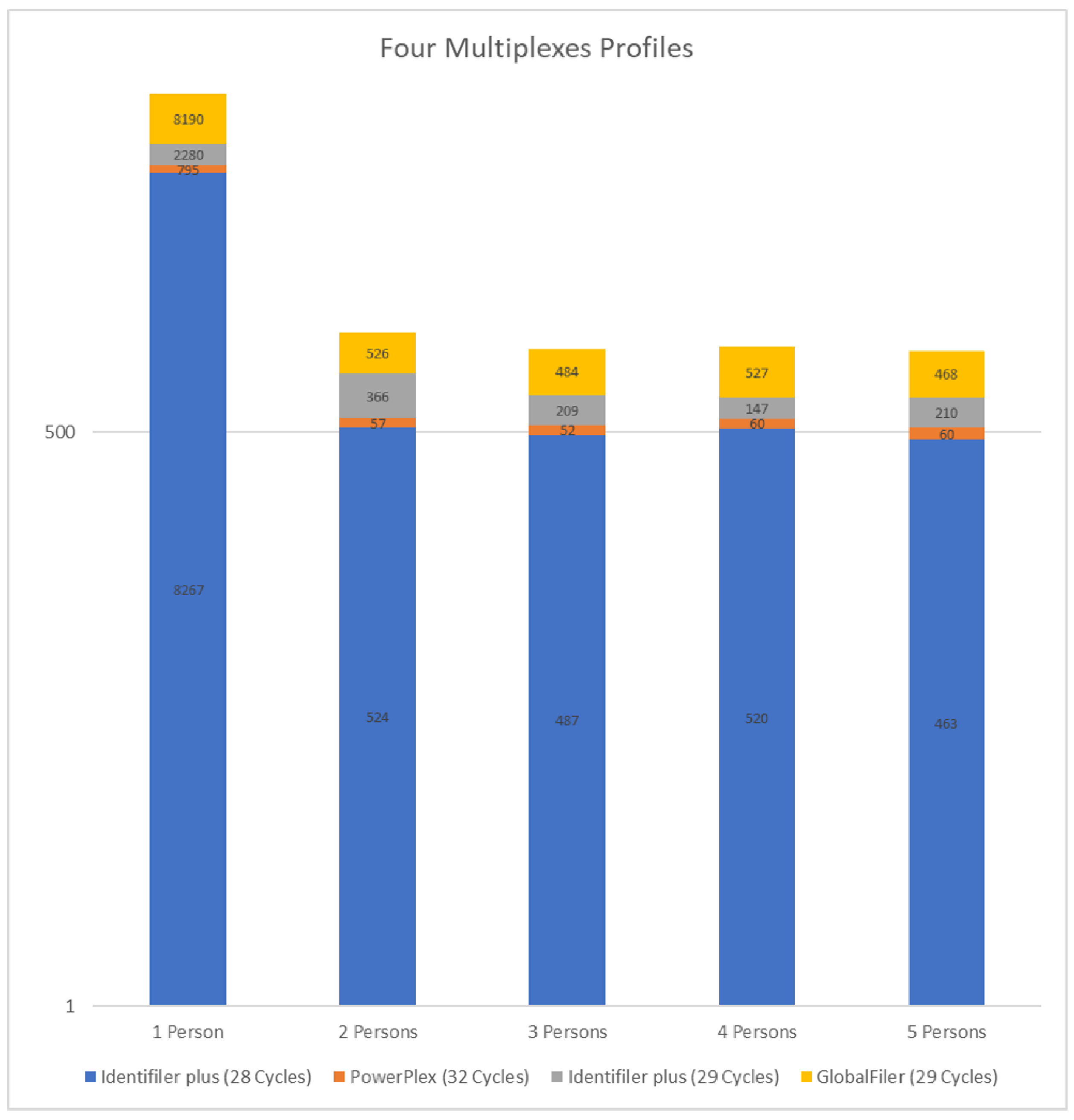
4.1.2. Four Multiplex Profiles (14 Loci)

In this scenario, we merged all the contents of the following multiplexes: Identifiler Plus (28 cycles), PowerPlex (32 cycles), Identifiler Plus (29 cycles), and GlobalFiler (29 cycles). Figure 15 shows that the minimum number of profiles is when profiles contain five persons (there are 1201 profiles), and the largest number of profiles is when profiles contain one person only (there are 19532 profiles). So, we took 1200 profiles from each group to end up with 6000 profiles (from different injection times), and the dataset was balanced.

4.1.3. Three Multiplexes Profiles (16 Loci)

In this scenario, we merged all the contents of the following multiplexes: Identifiler Plus (28 cycles), Identifiler Plus (29 cycles), and GlobalFiler (29 cycles). From Figure 16, we can see that the minimum number of profiles is when profiles contain five persons (there are 1141 profiles), and the largest number of profiles is when profiles contain one person only (there are 18,737 profiles). So, we took 1140 profiles from each group to end up with 5700 profiles (from different injection times), and the dataset was balanced.

4.2. Pre-Processing

In our case, we were interested in the filtered data. As a result of that, we dug further into it. Four folders are inside the filtered data folder; the difference between them is the different STR multiplexes used (the providers of the PROVEDIt dataset used three commercially available STR multiplexes: PowerPlex 16Hs, Identifiler Plus (28 cycles and 29 cycles), and GlobalFiler. Both PoerPlex 16Hs and Identifiler Plus co-amplify 15 STR loci plus the sex-determining Amelogenin locus. However, GlobalFiler amplifies 21 autosomal STRs, 1 Y-STR, 1 Y indel, and Amelogenin.

4.2.1. Data Imputation

First, let us demonstrate the markers for each multiplex in the PROVEDIt dataset (see

Table 3. The markers for the four multiplexes.

Identifiler Plus (28 Cycles)	Identifiler Plus (29 Cycles)	GlobalFiler (29 Cycles)	PowerPlex (32 Cycles)
D8S1179	D8S1179	D8S1179	D8S1179
D21S11	D21S11	D21S11	D21S11
D7S820	D7S820	D7S820	D7S820
CSF1PO	CSF1PO	CSF1PO	CSF1PO
D3S1358	D3S1358	D3S1358	D3S1358
TH01	TH01	TH01	TH01
D13S317	D13S317	D13S317	D13S317
D16S539	D16S539	D16S539	D16S539
D5S818	D5S818	D5S818	D5S818
D18S51	D18S51	D18S51	D18S51
vWA	vWA	vWA	vWA
TPOX	TPOX	TPOX	TPOX
FGA	FGA	FGA	FGA
AMEL	AMEL	AMEL	AMEL
D19S433	D19S433	D19S433	Penta D
D2S1338	D2S1338	D2S1338	Penta E
		SE33
		Yindel
		D22S1045
		D2S441
		D10S1248
		DAS1656
		D12S391
		DYS391

). Two questions appear looking at the table. 1. Is it better to use 14 markers from four multiplexes, or is it better to use 16 markers from three multiplexes only? 2. Or it is better to work with only one multiplex? In order to answer these questions, the manual balancing journey starts, because the imbalanced dataset appears when the number of examples in one class is more than the examples in other classes (in our case, the number of mixed profiles that contains only one contributor is more than the number of mixed profiles that contains two, three, four, and five contributors). We took a large subset from the dataset (we could not work with the whole dataset because the dataset is imbalanced). There are six challenges that we worked with; these are discussed in the next six subsections.

4.2.2. Missing Values

Most of the datasets could contain missing values that can affect model accuracy. The solution is to fill these missing values by calculating the mean/median and putting the values in the missing cells. The dataset contains values for 100 alleles (with their size and height). Figure 17 shows that almost half of the dataset contains null values. As a result of that, we dropped all the columns wherein almost all of it is a null value (we dropped the columns from allele 10 to allele height 100). Even when we dropped these columns, the null values challenge remained (see Figure 18). To deal with the null values, we created a missing indicator column for each column that contains missing values. Then, we filled the empty cells with the mean values because, in our proposed methodology, we deal with the missing values as a unique and significant mark for the sample.

4.2.3. Out of Ladder (OL) Values

As shown in the previous sections, the OL values are significant values that we need to show in the model. It is important to mention that the OL values appear only on the allele’s columns. To carry that out, we created a new column that is an indicator that shows where OL values are, and, in the same column, we put zero instead of the OL.

4.2.4. Amel, Yindel Loci, and Profile Name

In this experiment, we deleted both the Amel and Yindel loci (the single multiplex profiles contain both Amel and Yindel loci but the four multiplexes profiles (14 loci) and three multiplexes profiles (16 loci) contain just the Amel locus). By carrying that out, we had 22 markers for each sample instead of 24 markers in the single multiplex profiles, and 15 markers instead of 16 in the three multiplexes profiles (14 loci), and 13 loci in the four multiplexes profiles (14 loci). Note that we deleted the profile name column.

4.2.5. Dye Symbols and Marker Names

We dealt with both of these two columns as categorical features, and we converted them to numerical values.

4.2.6. Profile Loci

We created this feature because of its importance in specifying which markers are together (see

Table 4. Profile loci for the three scenarios.

Four Multiplex Profiles (14 Loci)	Three Multiplex Profiles (16 Loci)	Single Multiplex Profiles (24 Loci)
D8S1179	D8S1179	D8S1179
D21S11	D21S11	D21S11
D7S820	D7S820	D7S820
CSF1PO	CSF1PO	CSF1PO
D3S1358	D3S1358	D3S1358
TH01	TH01	TH01
D13S317	D13S317	D13S317
D16S539	D16S539	D16S539
D5S818	D5S818	D5S818
D18S51	D18S51	D18S51
vWA	vWA	vWA
TPOX	TPOX	TPOX
FGA	FGA	FGA
AMEL	AMEL	AMEL
	D19S433	D19S433
	D2S1338	D2S1338
		SE33
		Yindel
		D22S1045
		D2S441
		D10S1248
		DAS1656
		D12S391
		DYS391

).

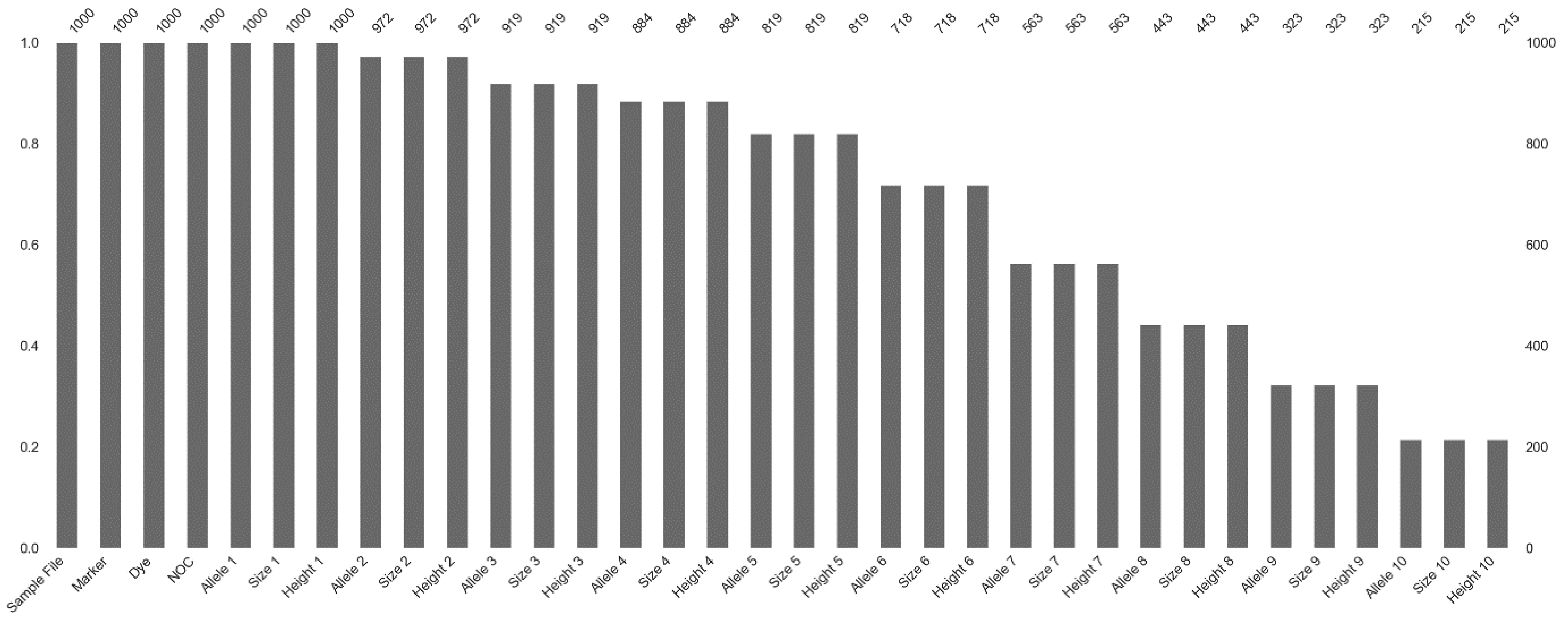
4.2.7. Feature Importance

Due to the fact that it is essential to know the features related to our dataset, we applied two techniques: the correlation matrix and univariate selection (to select the best features in the PROVEDIt dataset). For the correlation matrix, when looking at the documentation of this correlation, we found that the default method for calculating this correlation is the Pearson method, which is valid for continuous variables, and this meant that it is not valid for dummy variables (that have only two values (0 or 1). As a result of that, we removed all the dummy features and made the correlation. Figure 19 shows the correlation matrix for the single multiplex profiles (the correlation matrices for the two scenarios are similar and omitted for brevity). The features listed in these figures at the bottom of the figures from left to right are allele 1, size 1, height 1, allele 2, size 2, height 2, allele 3, size 3, height 3, allele 4, size 4, height 4, allele 5, size 5, height 5, allele 6, size 6, height 6, allele 7, size 7, height 7, allele 8, size 8, height 8, allele 9, size 9, height 9, allele 10, size 10, height 10, profile loci, and NOC. The positive correlations are depicted in the light and dark red colors, whereas the negative correlations are in the dark and light blue colors. The darker blue and darker red depict higher values of the correlations. The first thing that is observable from the correlations is that all of the features have a small and medium correlation with each other. For the target variable, we found that the profile loci feature has the largest positive correlation with it, and this is logical because the model needs this feature to know how many markers are in the profile. Some features are not correlated with the target. Instead, they are significantly correlated with other features, such as the allele’s size. From the heat map, we can see that each allele size has a strong correlation with the next allele. This correlation decreases when the alleles become far from each other.

Figure 20 shows the ten best features based on the Chi2 (compute chi-squared statistics between each non-negative feature and class) method. It shows that the profile loci, the OL indicators, and the indicator of the missing values play a vital role in all three scenarios.

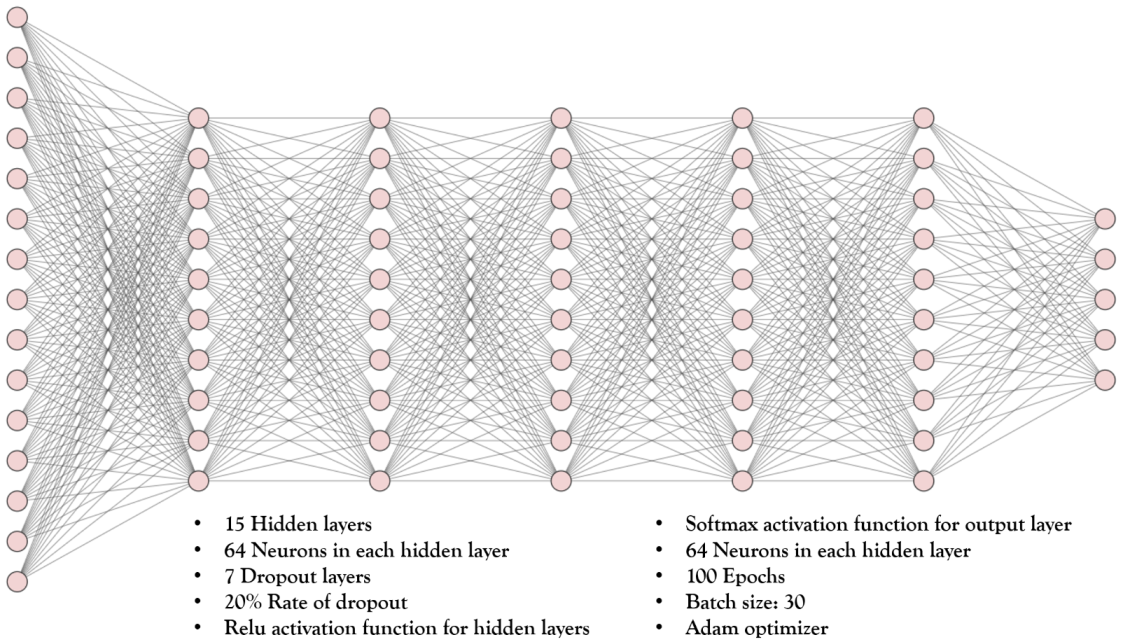
4.3. The Deep Learning Model

Subsequent to the pre-processing stage, we normalized all inputs to be distributed from [0,1]. We then split the dataset into a training set (70%) and a testing set (30%), and then we built a multi-Layer perceptron (MLP) model (see [37] to know more about the model). The model consists of 15 hidden layers (each layer contains 64 neurons), and between them, we added seven dropout layers (the dropout rate was 0.2). The last layer consists of five output nodes corresponding to the five classes we have. The activation function for all of the layers was relu, except for the output layer, which was softmax. After tweaking values, and some trial and error, we reached the configurations of the model that we have used in this paper. For more information about the set-up that was used, see

Table 5. MLP model configuration.

Specifications	Value
Number of hidden layers	15
Number of neurons in each hidden layer	64
Number of dropout layers	7
Rate of dropout	20%
The activation function for hidden layers	Relu
The activation function for the output layer	Softmax
The loss function	Categorical cross-entropy
Optimizer	adam
Epochs	100
Batch size	30

. Note that we chose MLP because it is suitable when dealing with tabular datasets. Due to the fact that the model’s performance depends on how the data are split, we needed to try different splits and to measure the performance at each trial. This could be carried out at the cross-validation stage. In this stage, the data were split into K parts, and, at each trial, one of these parts was used for testing, and the other K-1 parts were used for training. We applied cross-validation because it is a powerful preventative measure against overfitting, and it is used to avoid any dependency on the data split. We shuffled the training set randomly and split it into five groups. Then, we fitted the data to the model, and, finally, we made predictions and evaluated the model. Note that this experiment is the same for all three scenarios. We believe that our method deals with the challenge of finding the contributor number from a different perspective by benefiting from all of the information in the DNA profile, including the OL values and missing values. Figure 21 depicts the architecture of our MLP model.

4.4. Evaluation Metrics

We used four metrics—accuracy, precision, recall, and F1-score—for the evaluation. The formula is shown below. They are well-known metrics; TP stands for true positive, TN stands for true negative, FN stands for false negative, and FP stands for false positive.

• Accuracy shows how good the predictions are, on average.

  $$\mathrm{Accuracy}=(\mathrm{TP}+\mathrm{TN})/(\mathrm{TP}+\mathrm{FN}+\mathrm{TN}+\mathrm{FP});$$

  (1)
• Precision shows how accurate our model is out of those predicted positive, and how many of them are actual positive.

  $$\mathrm{Precision}=(\mathrm{TP}/(\mathrm{TP}+\mathrm{FP});$$

  (2)
• Recall shows how many of the actual positives our model captures through labeling it as positive.

  $$\mathrm{Recall}=\mathrm{TP}/(\mathrm{TP}+\mathrm{FN});$$

  (3)
• F1-score is the weighted average of precision and recall.

  $$\mathrm{F}1-\mathrm{Score}=2*(\mathrm{recall}*\mathrm{precision})/(\mathrm{recall}+\mathrm{precision}),$$

  (4)

5. Results and Analysis

This section presents the results and analysis. All scenarios were executed on a standard laptop computer with Intel(R)Core(TM) i7-8550U CPU@1.80GHz, 16GB RAM. Section 5.1, Section 5.2 and Section 5.3 discuss the results of single, four, and three multiplex profiles. Section 5.4 compares the performance of TAWSEEM with the related works.

5.1. The Single Multiplex Profiles

Figure 22 shows the confusion matrix for both the training and testing sets. From the figures, we can see that, for the training set, the four-contributor group has the largest number of misclassifications (259 sample-locus instances were classified as three contributors and 55 sample-locus instances were classified as five contributors). The three-contributor group has the least number of misclassifications (81 sample-locus instances were classified as two contributors and 25 sample-locus instances were classified as four contributors). For the testing set, the four-contributor group has the largest number of misclassifications (97 sample-locus instances were classified as three contributors, and 53 sample-locus instances were classified as five contributors), and the one-contributor group has the least number of misclassifications (61 sample-locus instances were classified as two contributors). The training set contains 546 profiles (12,012 sample-locus instances) and the testing set contains 234 profiles (5148 sample-locus instances).

Figure 23 shows the precision, recall, and F1-score for both training and testing sets. For the training set, the highest precision is found in the five-contributor group (0.98) and the least is for the three-contributor group (0.86). For recall, the highest score is in the three-contributor group (0.96) and the least is for the four-contributor group (0.87). For the F1-score, the highest score is in the one-contributor group (0.95), and the least is in the four-contributor group (0.88). For the testing set, the highest precision is in the one-contributor group and five-contributor group (0.95), and the least is in the three-contributor and four-contributor (0.84). For recall, the highest score is for the one-contributor group (0.94), and the least is for the four-contributor group (0.86). For the F1-score, the highest score is in the one-contributor (0.95), and the least is in three contributors and four contributors (0.85).

Figure 24 visualizes the prediction errors for both the training and testing set. From both figures, we can see that the one-contributor group can be misclassified as a two-contributor group, and the five-contributor group was misclassified as a four-contributor sample. The two, three, and four-contributor groups can be misclassified as lower contributors or higher contributors.

5.2. The Four Multiplexes Profiles (14 Loci)

Figure 25 shows the confusion matrix for both the training and testing sets. We note in the figure that, for the training set, the one-contributor group has the largest number of misclassifications (469 sample-locus instances were classified as two contributors), and the three-contributor group has the least number of misclassifications (five sample-locus instances were classified as two contributors and one sample-locus instance was classified as four contributors). For the testing set, the five-contributor group has the largest number of misclassification (193 sample-locus instances were classified as four contributors), and the three-contributor group has the least number of misclassification (15 sample-locus instances were classified as two contributors and 31 sample-locus instances were classified as four contributors). The training set contains 4200 profiles (54,600 sample-locus instances) and the testing set contains 1800 profiles (23,400 sample-locus instances).

Figure 26 shows the precision, recall, and F1-score for both the training and testing sets. For the training set, the highest precision is for both the one-contributor group and five-contributor group (1.0) and the least is for the two-contributor group (0.96). For recall, the highest score is for the three-contributor group and the least is for the one-contributor group (0.96). For the F1-score, the highest score is for the one-contributor, three-contributor, and five-contributor groups (0.98), and the least is for the two-contributor and four-contributor groups (0.97). For the testing set, the highest precision is for the one-contributor group (1.0), and the least is for the four-contributor group (0.95). For recall, the highest score is for the three-contributor group (0.99), and the least is for the five-contributor group (0.96). For the F1-score, the highest score is for the one-contributor group (0.99), and the least is for the four-contributor group (0.96). We did not plot the prediction errors for the four multiple profiles because they were similar to the prediction error plots of the single multiplex profiles, as in Figure 24.

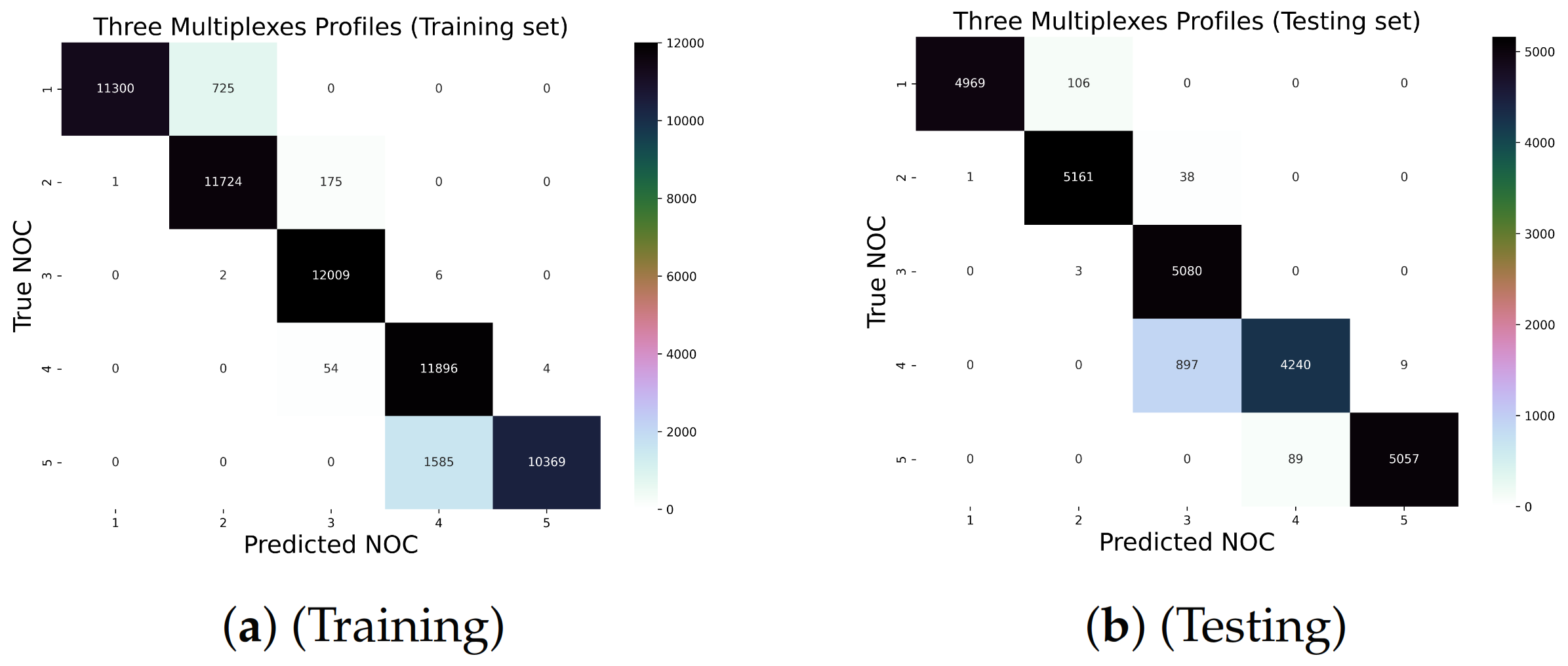
5.3. The Three Multiplex Profiles (16 Loci)

Figure 27 shows the confusion matrix for both the training and testing sets. From the figures, we can see that for the training set, the five-contributor group has the largest number of misclassifications (1585 sample-locus instances were classified as four contributors), and the three-contributor group has the least number of misclassifications (two sample-locus instances were classified as two contributors and six sample-locus instances were classified as four contributors). For the testing set, the four-contributor group has the largest number of misclassifications (897 sample-locus instances were classified as three contributors, and nine sample-locus instances were classified as five contributors), and the three-contributor group has the least number of misclassifications (three sample-locus instances were classified as two contributors). The training set contains 3990 profiles (59,850 sample-locus instances) and the testing set contains 1710 profiles (25,650 sample-locus instances).

Figure 28 shows the precision, recall, and F1-score for both the training and testing datasets. For the training set, the highest precision is for both the one-contributor group and five-contributor group (1.0) and the least is for the four-contributor group (0.88). For recall, the highest score is for the three-contributor group and the four-contributor group, and the least is for the five-contributor group (0.87). For the F1-score, the highest score is for the three-contributor group (0.99), and the least is for the five-contributor group (0.93). For the testing set, the highest precision is for the one-contributor group and five-contributor group (1.0), and the least is for the three-contributor group (0.84). For recall, the highest score is for the three-contributor group (1.0), and the least is for the four-contributor group (0.82). For the F1-score, the highest score is for the one-contributor, two-contributor, and five-contributor groups (0.99), and the least is for the four-contributor group (0.89). We did not plot the prediction errors for the three multiple profiles because they were similar to the prediction error plots of the single multiplex profiles, as in in Figure 24.

Figure 29 shows the accuracy for the three scenarios. The TAWSEEM small dataset has the least accuracy among the other scenarios, and the TAWSEEM four multiplexes profiles (14 loci) has the highest accuracy among the other scenarios. The difference between these scenarios is in the profiles and marker numbers. TAWSEEM contains the largest number of markers among the three scenarios. However, it contains the least number of profiles. In contrast, the 14 loci contain the least number of markers and the largest number of profiles. The 16 loci are in the middle (in terms of the marker and profiles number). From the results, we can see the effect of making the model train on a large amount of data.

5.4. TAWSEEM: Comparison with Other Works

Table 6. TAWSEEM: comparison with other machine-learning-based works.

Research	Profiles	Method	Features	Accuracy
RFC19 [13] (2019)	590	RFC	19	0.83
Kruijver [15] (2021)	766	DT	-	0.77–0.85
TAWSEEM (2022)	6000	MLP	75	0.97

shows a comparison between our proposed model and the related works. The first column gives the reference for the research. Column 2 gives the number of profiles. Column 3 lists the name of the ML method that has been used. Column 4 lists the number of features used in the respective works. Column 5 gives the reported accuracy of the respective works. For the first work (RFC19 [13]), the authors used 590 profiles to test their RFC model with 19 features. The accuracy was 0.83. For the second work, the authors used 766 profiles with the decision tree, and the reported accuracy range was 0.77–0.85. For our work, we list the results for the largest dataset, i.e., four multiplex profiles containing 6000 features. We used the MLP DL model. The accuracy for this case was 0.97. The accuracy is the highest among all the works that considered up to five contributors.

A further comparison of TAWSEEM with the competing works, with regard to the number of contributors, profiles, and loci, follows. For the number of contributors, PACE [12] considered four contributors. RFC19 [13], Kruijver et al. [15], and this work considered DNA mixtures with one to five contributors. For the number of profiles, PACE considered 1405 profiles, RFC19 [13] considered 590 profiles, and Kruijver et al. [15] considered 766 profiles. We considered three different scenarios with a different number of mixture profiles; single multiplex with 780 profiles, three multiplexes with 5700 profiles, and four multiplexes with 6000 profiles. For the number of loci, PACE considered 15 loci, RFC19 [13] considered 23 loci, and Kruijver et al. [15] did not mention the number of loci they used. In our work, we used three different scenarios with different loci numbers: single multiplex profiles have 22 loci, three multiplex profiles have 15 loci, and four multiplex profiles have 13 loci. For the models that have been used, PACE used SVM, RFC19 [13] used RFC, Kruijver et al. [15] used decision trees, and we used MLP.

Figure 30 plots the execution times for our deep learning model. The execution times are for each dataset profile we used in this paper. The average of the times of the three dataset profiles is also plotted. We have mentioned earlier that there are only four works that can be considered competitors to our work. These works have used different datasets or different numbers of data profiles in their experiments and, therefore, the execution times can vary because of these and other dataset attributes. These works either have not reported the execution times of their models or the reported times have not been clearly specified. Moreover, the use of different computing hardware also makes it difficult to compare the work. The only work that has clearly stated the time is PACE by Marciano et al. [12]. We have discussed this work already in the literature review section (Section 3). The authors reported that their model took around 90 min for training and testing on an Intel Core i5 machine. However, they considered up to four contributors and a smaller dataset, and, therefore, its time cannot be directly compared with our tool (and the other works that considered five contributors).

6. Conclusions and Future Work

Research in DNA profiling is important due to its several crucial applications, such as criminal investigations, paternity tests, disaster victim identification, missing person investigations, and mapping genetic diseases. A crucial task in DNA profiling is identifying the number of contributors in a DNA mixture profile, which is challenging due to issues that include allele dropout, stutter, blobs, noise in DNA profiles, estimation accuracy, and computational complexity. The existing work on machine-learning-based methods for estimating the number of unknowns is limited, needing many more efforts to develop robust models and their training on large and diverse datasets.

In this paper, we proposed and developed a software tool called TAWSEEM that employs a multilayer perceptron (MLP) neural network deep learning model for estimating the number of unknown contributors in DNA mixture profiles using PROVEDIt, the largest publicly available dataset. We investigate the performance of our developed deep learning model using four performance metrics, namely accuracy, F1-score, recall, and precision. This is a novel and significant contribution to the DNA profiling field because the tool provides the highest accuracy (97%) and a detailed account of the deep learning tool development and the performance investigation of the deep learning method across various multiplexes, loci, and profiles. Such modeling details and the analysis of results have not been reported in any other DNA profiling works.

In the future, it is expected that the number of genetic markers will increase, requiring software tools with a good accuracy and high speed. The results so far have been promising; however, further research in several directions is needed. Firstly, we have attempted to make good use of the DNA profile information by applying data pre-processing methods and dealing with both the OL and missing values as a significant position in the profile, which we believe is one of our work’s strengths. Further work in feature engineering methods for estimating the number of contributors is needed. Secondly, we tested our model on the PROVEDIt dataset. Further investigation is needed to understand the performance of the machine and deep learning methods over diverse datasets and profile characteristics, such as dealing with imbalanced datasets, variations in the numbers of loci, injection times, cycle numbers, wrong profile labels (a mixture with five contributors labeled as a mixture with two contributors), and different dataset formats (image versus numeric DNA profile data).

Thirdly, publicly available DNA-profiling-related datasets are limited. More DNA profile datasets are needed to study the generalizability of AI methods. Finally, the work is part of our broader work on DNA profiling, with our earlier contribution of the first distributed-memory HPC implementations [11] of DNA profiling using maximum likelihood ratio computations and reporting results for up to ten unknowns delivering over 15x the performance using over 3000 cores. We plan to excel and work towards developing research in complete genome-sequencing-based DNA profile and information systems that integrate DNA-profile-level information with higher-level healthcare and environment information. This will involve integrating our existing strands of work on DNA profiling with other research in healthcare, high performance computing [38,39], big data [40], smart analytics [41], enterprise and information systems, cloud, fog, and edge computing [42], and smart cities [43,44].

The software tool and the deep learning model developed in this work can be implemented in hardware, such as on a field programmable gate arrays (FPGA) device, in order to develop specialized and faster stand-alone devices for DNA profiling, and we hope that the community will investigate this. Moreover, in this work, we used MLP; however, there are several other deep learning networks, such as long short-term memory (LSTM) and generative adversarial networks (GANs), that are known to have provided better performance in other applications [45,46,47,48]. Future work will focus on using those deep learning networks.

References

1. Butler, J.M. Fundamentals of Forensic DNA Typing; Elsevier Inc.: Amsterdam, The Netherlands, 2010. [Google Scholar] [CrossRef]
2. Alamoudi, E.; Mehmood, R.; Albeshri, A.; Gojobori, T. A Survey of Methods and Tools for Large-Scale DNA Mixture Profiling. In Smart Infrastructure and Applications; Springer: Cham, Switzerland, 2020; pp. 217–248. [Google Scholar] [CrossRef]
3. Clayton, T.M.; Whitaker, J.P.; Sparkes, R.; Gill, P. Analysis and interpretation of mixed forensic stains using DNA STR profiling. Forensic Sci. Int. 1998, 91, 55–70. [Google Scholar] [CrossRef]
4. Egeland, T.; Dalen, I.; Mostad, P.F. Estimating the number of contributors to a DNA profile. Int. J. Leg. Med. 2003, 117, 271–275. [Google Scholar] [CrossRef] [PubMed]
5. Taylor, D.; Bright, J.A.; Buckleton, J. Interpreting forensic DNA profiling evidence without specifying the number of contributors. Forensic Sci. Int. Genet. 2014, 13, 269–280. [Google Scholar] [CrossRef] [PubMed]
6. Alotaibi1, H.; Alsolami, F.; Mehmood, R. DNA Profiling: An Investigation of Six Machine Learning Algorithms for Estimating the Number of Contributors in DNA Mixtures. Int. J. Adv. Comput. Sci. Appl. (IJACSA) 2021, 12. [Google Scholar] [CrossRef]
7. Swaminathan, H.; Grgicak, C.M.; Medard, M.; Lun, D.S. NOCIt: A computational method to infer the number of contributors to DNA samples analyzed by STR genotyping. Forensic Sci. Int. Genet. 2015, 16, 172–180. [Google Scholar] [CrossRef]
8. Alamoudi, E.; Mehmood, R.; Albeshri, A.; Gojobori, T. DNA Profiling Methods and Tools: A Review. In International Conference on Smart Cities, Infrastructure, Technologies and Applications; Springer: Cham, Switzerland, 2018. [Google Scholar] [CrossRef]
9. Bleka, Ø.; Storvik, G.; Gill, P. EuroForMix: An open source software based on a continuous model to evaluate STR DNA profiles from a mixture of contributors with artefacts. Forensic Sci. Int. Genet. 2016, 21, 35–44. [Google Scholar] [CrossRef] [Green Version]
10. Balding, D.J.; Steele, C.D.; Building, D.; Street, G. likeLTD v6.3: An Illustrative Analysis, Explanation of the Model, Results of Validation Tests and Version History. Available online: https://blogs.unimelb.edu.au/statisticalgenomics/publications-software/likeltd-software/ (accessed on 5 February 2022).
11. Alamoudi, E.M. Parallel Analysis of DNA Profile Mixtures with a Large Number of Contributors. Master’s Thesis, King Abdulaziz University, Jeddah, Saudi Arabia, 2019. [Google Scholar]
12. Marciano, M.A.; Adelman, J.D. PACE: Probabilistic Assessment for Contributor Estimation—A machine learning-based assessment of the number of contributors in DNA mixtures. Forensic Sci. Int. Genet. 2017, 27, 82–91. [Google Scholar] [CrossRef]
13. Benschop, C.C.G.; Linden, J.V.; Hoogenboom, J.; Ypma, R.; Haned, H. Automated estimation of the number of contributors in autosomal short tandem repeat profiles using a machine learning approach. Forensic Sci. Int. Genet. 2019, 1–33. [Google Scholar] [CrossRef]
14. Alfonse, L.E.; Garrett, A.D.; Lun, D.S.; Duffy, K.R.; Grgicak, C.M. A large-scale dataset of single and mixed-source short tandem repeat profiles to inform human identification strategies: PROVEDIt. Forensic Sci. Int. Genet. 2018, 32, 62–70. [Google Scholar] [CrossRef]
15. Kruijver, M.; Kelly, H.; Cheng, K.; Lin, M.H.; Morawitz, J.; Russell, L.; Buckleton, J.; Bright, J.A. Estimating the number of contributors to a DNA profile using decision trees. Forensic Sci. Int. Genet. 2021, 50, 102407. [Google Scholar] [CrossRef]
16. Coquoz, R. FORENSIC SCIENCES|DNA Profiling. Encycl. Anal. Sci. 2005, 384–391. [Google Scholar] [CrossRef]
17. Graversen, T. Statistical and Computational Methodology for the Analysis of Forensic DNA Mixtures with Artefacts. Ph.D. Thesis, Oxford University, Oxford, UK, 2014; p. 229. [Google Scholar]
18. Garofano, P.; Caneparo, D.; D’Amico, G.; Vincenti, M.; Alladio, E. An alternative application of the consensus method to DNA typing interpretation for Low Template-DNA mixtures. Forensic Sci. Int. Genet. Suppl. Ser. 2015, 5, e422–e424. [Google Scholar] [CrossRef]
19. Fedushko, S.; Ustyianovych, T.; Gregus, M. Real-Time High-Load Infrastructure Transaction Status Output Prediction Using Operational Intelligence and Big Data Technologies. Electronics 2020, 9, 668. [Google Scholar] [CrossRef] [Green Version]
20. Alam, F.; Almaghthawi, A.; Katib, I.; Albeshri, A.; Mehmood, R. iResponse: An AI and IoT-Enabled Framework for Autonomous COVID-19 Pandemic Management. Sustainability 2021, 13, 3797. [Google Scholar] [CrossRef]
21. Muhammed, T.; Mehmood, R.; Albeshri, A.; Katib, I. UbeHealth: A personalized ubiquitous cloud and edge-enabled networked healthcare system for smart cities. IEEE Access 2018, 6, 32258–32285. [Google Scholar] [CrossRef]
22. Alomari, E.; Katib, I.; Albeshri, A.; Yigitcanlar, T.; Mehmood, R. Iktishaf+: A Big Data Tool with Automatic Labeling for Road Traffic Social Sensing and Event Detection Using Distributed Machine Learning. Sensors 2021, 21, 2993. [Google Scholar] [CrossRef]
23. Omar Alkhamisi, A.; Mehmood, R. An Ensemble Machine and Deep Learning Model for Risk Prediction in Aviation Systems. In 2020 6th Conference on Data Science and Machine Learning Applications (CDMA); Institute of Electrical and Electronics Engineers (IEEE): Riyadh, Saudi Arabia, 2020; pp. 54–59. [Google Scholar] [CrossRef]
24. Aqib, M.; Mehmood, R.; Alzahrani, A.; Katib, I.; Albeshri, A.; Altowaijri, S.M. Rapid Transit Systems: Smarter Urban Planning Using Big Data, In-Memory Computing, Deep Learning, and GPUs. Sustainability 2019, 11, 2736. [Google Scholar] [CrossRef] [Green Version]
25. Mehmood, R.; Alam, F.; Albogami, N.N.; Katib, I.; Albeshri, A.; Altowaijri, S.M. UTiLearn: A Personalised Ubiquitous Teaching and Learning System for Smart Societies. IEEE Access 2017, 5, 2615–2635. [Google Scholar] [CrossRef]
26. Mehmood, R.; See, S.; Katib, I.; Chlamtac, I. Smart Infrastructure and Applications: Foundations for Smarter Cities and Societies; Springer International Publishing; Springer Nature: Cham, Switzerland, 2020; p. 692. [Google Scholar] [CrossRef]
27. Yigitcanlar, T.; Kankanamge, N.; Regona, M.; Maldonado, A.R.; Rowan, B.; Ryu, A.; Desouza, K.C.; Corchado, J.M.; Mehmood, R.; Li, R.Y.M. Artificial Intelligence Technologies and Related Urban Planning and Development Concepts: How Are They Perceived and Utilized in Australia? J. Open Innov. Technol. Mark. Complex. 2020, 6, 187. [Google Scholar] [CrossRef]
28. Yigitcanlar, T.; Regona, M.; Kankanamge, N.; Mehmood, R.; D’Costa, J.; Lindsay, S.; Nelson, S.; Brhane, A. Detecting Natural Hazard-Related Disaster Impacts with Social Media Analytics: The Case of Australian States and Territories. Sustainability 2022, 14, 810. [Google Scholar] [CrossRef]
29. Alam, F.; Mehmood, R.; Katib, I.; Albogami, N.N.; Albeshri, A. Data Fusion and IoT for Smart Ubiquitous Environments: A Survey. IEEE Access 2017, 5, 9533–9554. [Google Scholar] [CrossRef]
30. Mohammed, T.; Albeshri, A.; Katib, I.; Mehmood, R. DIESEL: A Novel Deep Learning based Tool for SpMV Computations and Solving Sparse Linear Equation Systems. J. Supercomput. 2020, 77, 6313–6355. [Google Scholar] [CrossRef]
31. Muhammed, T.; Mehmood, R.; Albeshri, A.; Katib, I. SURAA: A novel method and tool for loadbalanced and coalesced SpMV computations on GPUs. Appl. Sci. 2019, 9, 947. [Google Scholar] [CrossRef] [Green Version]
32. Bosaeed, S.; Katib, I.; Mehmood, R. A Fog-Augmented Machine Learning based SMS Spam Detection and Classification System. In Proceedings of the 2020 Fifth International Conference on Fog and Mobile Edge Computing (FMEC), Paris, France, 20–23 April 2020; pp. 325–330. [Google Scholar] [CrossRef]
33. Gustisyaf, A.I.; Sinaga, A. Implementation of Convolutional Neural Network to Classification Gender based on Fingerprint. Int. J. Mod. Educ. Comput. Sci. (IJMECS) 2021, 13, 55–67. [Google Scholar] [CrossRef]
34. Hung, C.L.; Tang, C.Y. Bioinformatics tools with deep learning based on GPU. In Proceedings of the 2017 IEEE International Conference on Bioinformatics and Biomedicine (BIBM), Kansas City, MO, USA, 13–16 November 2017; pp. 1906–1908. [Google Scholar] [CrossRef]
35. Larranaga, P.; Calvo, B.; Santana, R.; Bielza, C.; Galdiano, J.; aki Inza, I.; Lozano, A.; Anzas, A.; Pe, A.; Robles, V.; et al. Machine learning in bioinformatics Downloaded from. Briefings Bioinform. 1991, 7, 112. [Google Scholar] [CrossRef] [Green Version]
36. Olson, R.S.; La Cava, W.; Mustahsan, Z.; Varik, A.; Moore, J.H. Data-driven advice for applying machine learning to bioinformatics problems. Pac. Symp. Biocomput. 2018, 0, 192–203. [Google Scholar] [CrossRef] [Green Version]
37. Schmauch, B.; Romagnoni, A.; Pronier, E.; Saillard, C.; Maillé, P.; Calderaro, J.; Kamoun, A.; Sefta, M.; Toldo, S.; Zaslavskiy, M.; et al. A deep learning model to predict RNA-Seq expression of tumours from whole slide images. Nat. Commun. 2020, 11, 3877. [Google Scholar] [CrossRef] [PubMed]
38. AlAhmadi, S.; Mohammed, T.; Albeshri, A.; Katib, I.; Mehmood, R. Performance Analysis of Sparse Matrix-Vector Multiplication (SpMV) on Graphics Processing Units (GPUs). Electronics 2020, 9, 1675. [Google Scholar] [CrossRef]
39. Alyahya, H.; Mehmood, R.; Katib, I. Parallel Iterative Solution of Large Sparse Linear Equation Systems on the Intel MIC Architecture. In Smart Infrastructure and Applications; Springer: Cham, Switzerland, 2020; pp. 377–407. [Google Scholar] [CrossRef]
40. Usman, S.; Mehmood, R.; Katib, I. Big Data and HPC Convergence for Smart Infrastructures: A Review and Proposed Architecture. EAI/Springer Innov. Commun. Comput. 2020, 561–586. [Google Scholar] [CrossRef]
41. Alotaibi, S.; Mehmood, R.; Katib, I. Sentiment analysis of Arabic tweets in smart cities: A review of Saudi dialect. In Proceedings of the 2019 4th International Conference on Fog and Mobile Edge Computing, Rome, Italy, 10–13 June 2019. [Google Scholar] [CrossRef]
42. Mohammed, T.; Albeshri, A.; Katib, I.; Mehmood, R. UbiPriSEQ—Deep Reinforcement Learning to Manage Privacy, Security, Energy, and QoS in 5G IoT HetNets. Appl. Sci. 2020, 10, 7120. [Google Scholar] [CrossRef]
43. Yigitcanlar, T.; Mehmood, R.; Corchado, J.M. Green Artificial Intelligence: Towards an Efficient, Sustainable and Equitable Technology for Smart Cities and Futures. Sustainability 2021, 13, 8952. [Google Scholar] [CrossRef]
44. Yigitcanlar, T.; Corchado, J.M.; Mehmood, R.; Li, R.Y.M.; Mossberger, K.; Desouza, K. Responsible Urban Innovation with Local Government Artificial Intelligence (AI): A Conceptual Framework and Research Agenda. J. Open Innov. Technol. Mark. Complex. 2021, 7, 71. [Google Scholar] [CrossRef]
45. Yan, X.; Cui, B.; Xu, Y.; Shi, P.; Wang, Z. A Method of Information Protection for Collaborative Deep Learning under GAN Model Attack. IEEE/ACM Trans. Comput. Biol. Bioinform. 2021, 18, 871–881. [Google Scholar] [CrossRef]
46. Li, X.; Du, Z.; Huang, Y.; Tan, Z. A deep translation (GAN) based change detection network for optical and SAR remote sensing images. ISPRS J. Photogramm. Remote. Sens. 2021, 179, 14–34. [Google Scholar] [CrossRef]
47. Leka, H.L.; Fengli, Z.; Kenea, A.T.; Tegene, A.T.; Atandoh, P.; Hundera, N.W. A Hybrid CNN-LSTM Model for Virtual Machine Workload Forecasting in Cloud Data Center. In Proceedings of the 2021 18th International Computer Conference on Wavelet Active Media Technology and Information Processing (ICCWAMTIP), Chengdu, China, 17–19 December 2021; pp. 474–478. [Google Scholar]
48. De Oliveira, L.T.; Colaço, M.; Prado, K.H.; de Oliveira, F.R. A Big Data Experiment to Evaluate the Effectiveness of Traditional Machine Learning Techniques Against LSTM Neural Networks in the Hotels Clients Opinion Mining. In Proceedings of the 2021 IEEE International Conference on Big Data (Big Data), Orlando, FL, USA, 15–18 December 2021; pp. 5199–5208. [Google Scholar]
Figure 1. Comparison of printed and genetic information.
Electronics 11 00548 g001
Figure 2. Difference between heterozygous and homozygous alleles.
Electronics 11 00548 g002
Figure 3. Male DNA profile.
Electronics 11 00548 g003
Figure 4. Female DNA profile.
Electronics 11 00548 g004
Figure 5. Two-person mixture DNA profile.
Electronics 11 00548 g005
Figure 6. Single vs. mixed sample.
Electronics 11 00548 g006
Figure 7. Possible genotype combinations in two-person mixture.
Electronics 11 00548 g007
Figure 8. A base pair (size of DNA is measured by its base pairs) and dropout.
Electronics 11 00548 g008
Figure 9. Short tandem repeats (STRs).
Electronics 11 00548 g009
Figure 10. Rarity estimation.
Electronics 11 00548 g010
Figure 11. TAWSEEM: a high-level view.
Electronics 11 00548 g011
Figure 12. The PROVEDIt dataset.
Electronics 11 00548 g012
Figure 13. The number of profiles for Identifiler Plus multiplex.
Electronics 11 00548 g013
Figure 14. The number of profiles for PowerPlex and GlobalFiler multiplexes.
Electronics 11 00548 g014
Figure 15. The four multiplexes profiles (14 loci).
Electronics 11 00548 g015
Figure 16. The three multiplexes profiles (16 loci).
Electronics 11 00548 g016
Figure 17. The null values in the dataset.
Electronics 11 00548 g017
Figure 18. The resultant dataset.
Electronics 11 00548 g018
Figure 19. The correlation matrix (single multiplex profiles).
Electronics 11 00548 g019
Figure 20. Feature importance: single, three, and four multiplex profiles.
Electronics 11 00548 g020
Figure 21. MLP architecture.
Electronics 11 00548 g021
Figure 22. TAWSEEM: training and testing confusion matrices (single multiplex profiles).
Electronics 11 00548 g022
Figure 23. TAWSEEM: precision, recall, and F1 score (single multiplex profiles).
Electronics 11 00548 g023
Figure 24. TAWSEEM: prediction errors (single multiplex profiles).
Electronics 11 00548 g024
Figure 25. TAWSEEM: confusion matrix (four multiplex profiles).
Electronics 11 00548 g025
Figure 26. TAWSEEM: precision, recall and F1 score (four multiplexes profiles).
Electronics 11 00548 g026
Figure 27. TAWSEEM: confusion matrix (three multiplexes profiles).
Electronics 11 00548 g027
Figure 28. TAWSEEM: precision, recall, and F1-score (three multiplexes profiles).
Electronics 11 00548 g028
Figure 29. Prediction accuracy: comparison of single, three, and four multiplex profiles.
Electronics 11 00548 g029
Figure 30. TAWSEEM: execution times.
Electronics 11 00548 g030