
Reservation-Based 3D Intersection Traffic Control System for Autonomous Unmanned Aerial Vehicles

Abstract
:1. Introduction
2. Related Work
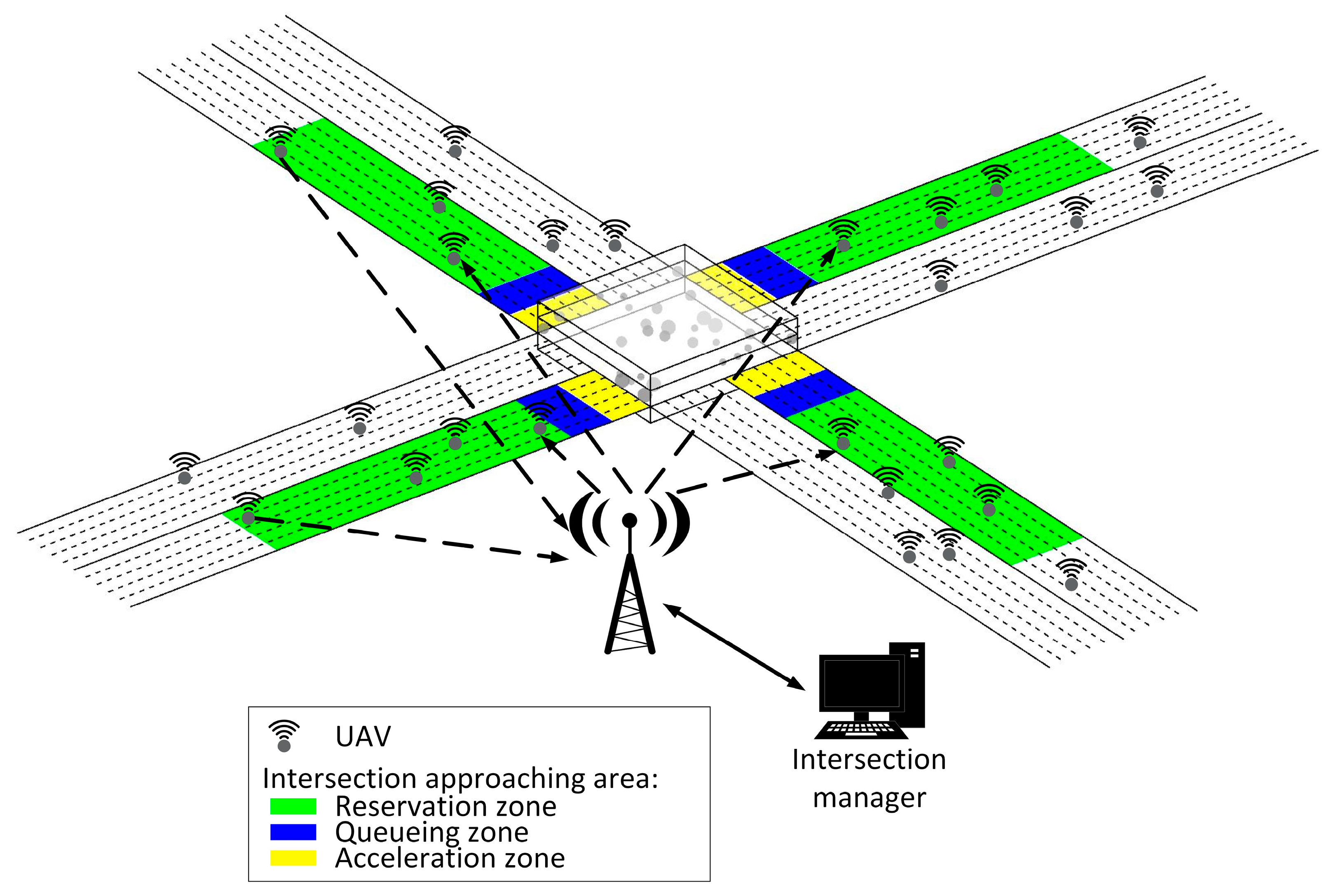
3. System Model
- It cannot change lanes
- It cannot overtake a UAV ahead
- It must travel at constant altitude
- It must maintain its speed within [, ], unless it needs to slow down to avoid collision with UAV ahead or delay its entrance to the intersection. We will discuss in Section 4 how a UAV will decide its speed such that it can avoid collision with a UAV ahead and enter the intersection as scheduled.
- It must send reservation request to the intersection manager as soon as it enters the reservation zone. A reservation request message contains the UAV ID, time the request was sent, UAV’s position when it sent the request, UAV’s lane, and UAV’s size.
- It enters the acceleration zone such that it can enter the intersection as scheduled.
- Reservation zone
- Queueing zone
- Acceleration zone
4. UAV’s Behavior in the Approaching Area
- (1)
- is in the reservation zone
- (a)
- is in the reservation zone or queueing zone
- (b)
- is in the acceleration zone
- (2)
- is in the queueing zone
- (a)
- is in the queueing zone
- (b)
- is in the acceleration zone
- (3)
- is in acceleration zone
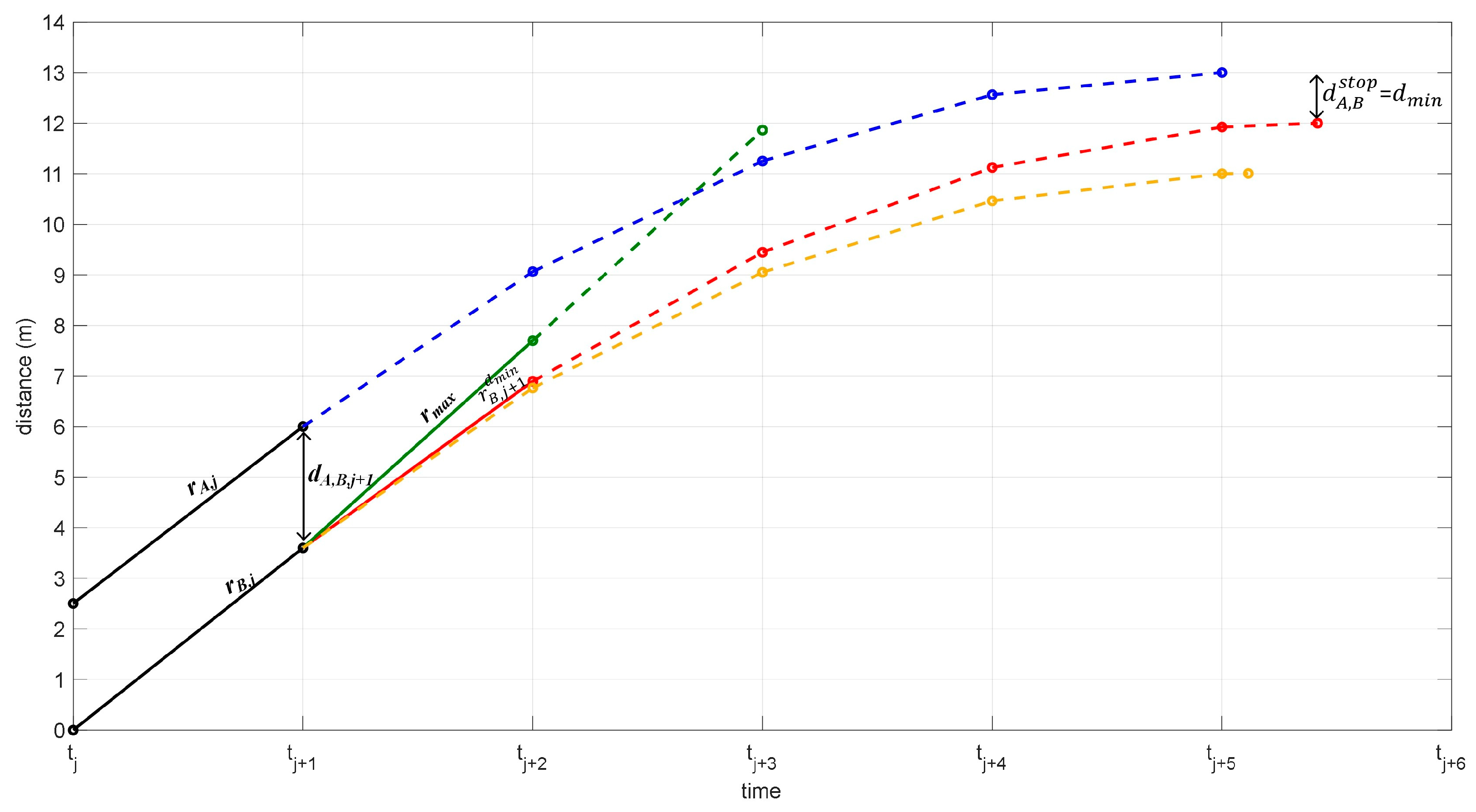
4.1. Avoiding Collision with a UAV Ahead
4.2. Entering the Intersection as Scheduled
- Scenarios for which is less than zero
- ∘
- Scenario 1: slows down at rate from until it reaches the entrance of the acceleration zone. It reaches the entrance of acceleration zone with speed equal to zero. Then, it waits for some time before it enters the acceleration zone. In the acceleration zone, it accelerates at rate until its speed reaches . Then, it maintains its speed until it enters the intersection.
- ∘
- Scenario 2: slows down at rate from until it reaches the entrance of the acceleration zone with speed equal to zero. Then, it immediately enters the acceleration zone and then accelerates at rate until its speed reaches . Then, it maintains its speed until it enters the intersection.
- ∘
- Scenario 3: slows down at rate from until it reaches the entrance of the acceleration zone. It reaches the entrance of acceleration zone with speed greater than zero. Then, it enters the acceleration zone and accelerates at rate until its speed reaches . Then, it maintains its speed until it enters the intersection.
- Scenarios for which is equal to zero
- ∘
- Scenario 4: maintains its speed in the queueing zone, which is less than . Then, it enters the acceleration zone and accelerates at rate until its speed reaches . Then, it maintains its speed until it enters the intersection.
- ∘
- Scenario 5: maintains its speed in the queueing zone, which is equal to . Then, it enters the acceleration zone and maintains its speed until it enters the intersection.
- Scenarios for which is greater than zero
- ∘
- Scenario 6: accelerates at rate from until it reaches the entrance of the acceleration zone. It reaches the entrance of the acceleration zone with speed less than . In the acceleration zone, it accelerates at rate until its speed reaches . Then, it maintains its speed until it enters the intersection.
- ∘
- Scenario 7: accelerates in the queueing zone at rate from until it reaches the entrance of the acceleration zone with speed equal to . Then, it maintains its speed until it enters the intersection.
- (1)
- (2)
- (3)
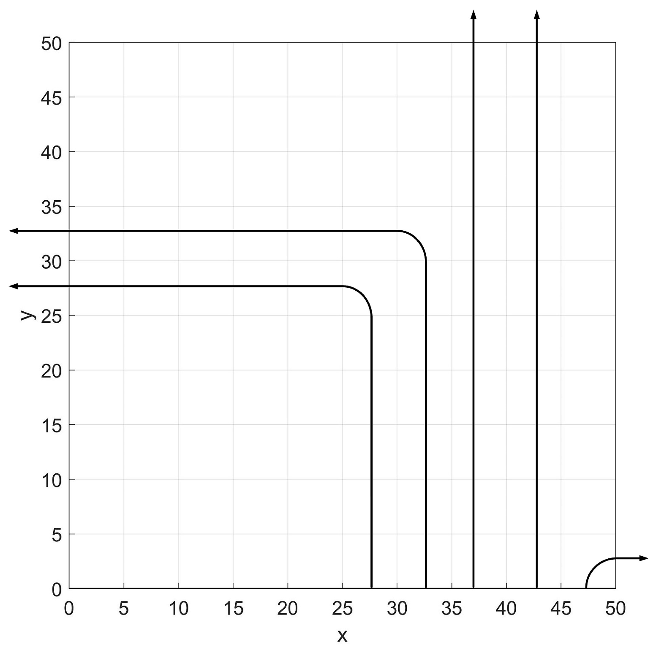
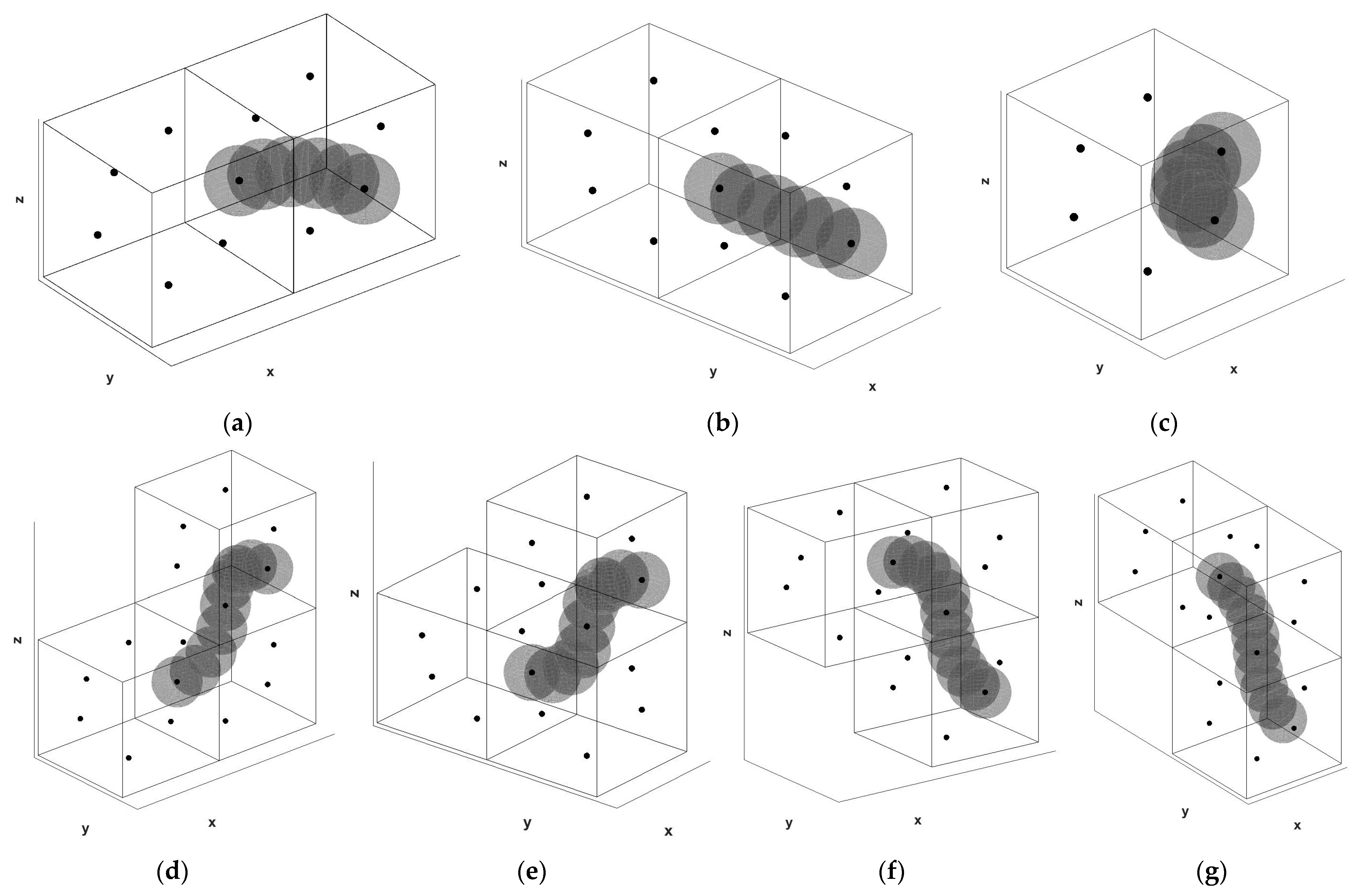
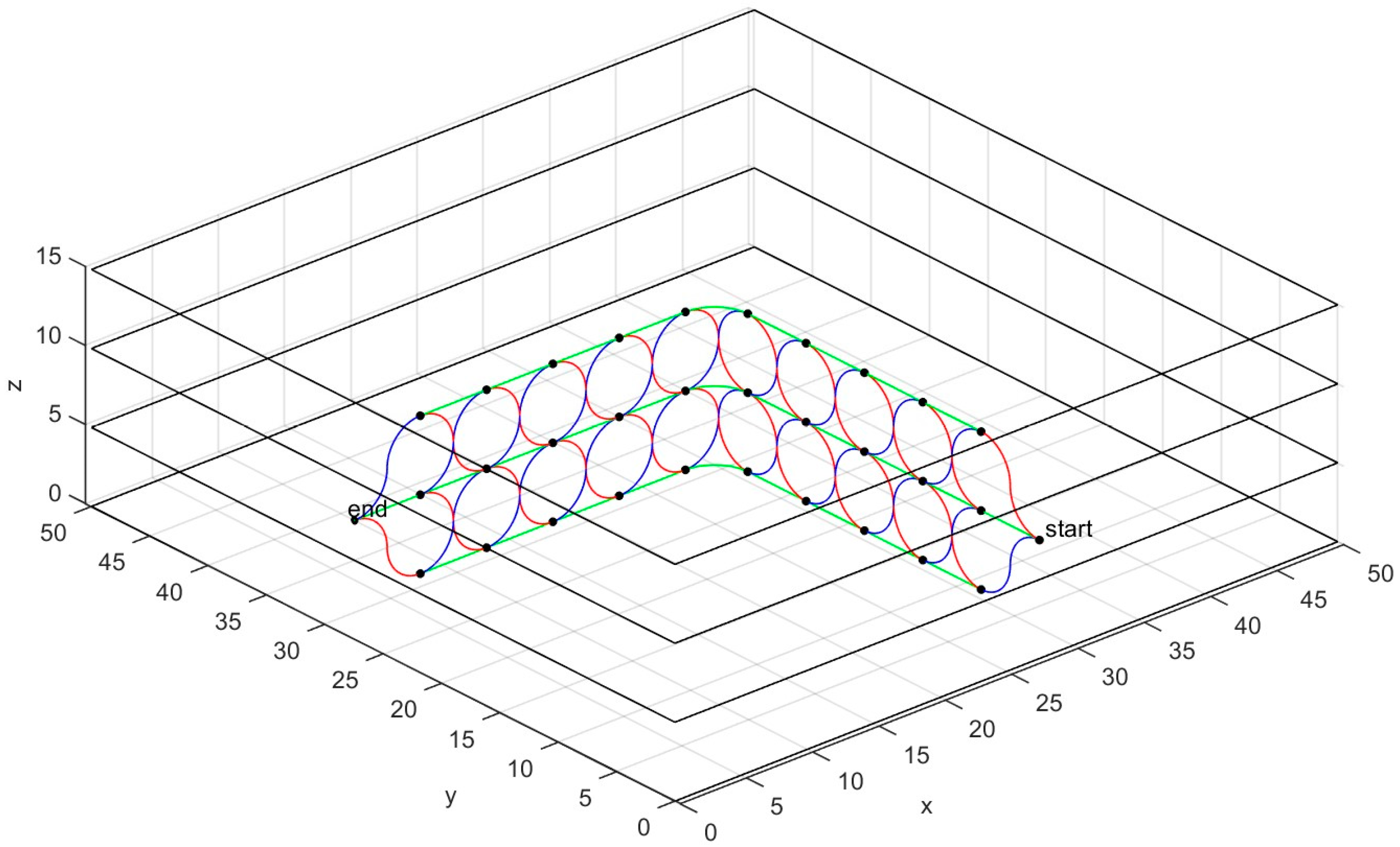
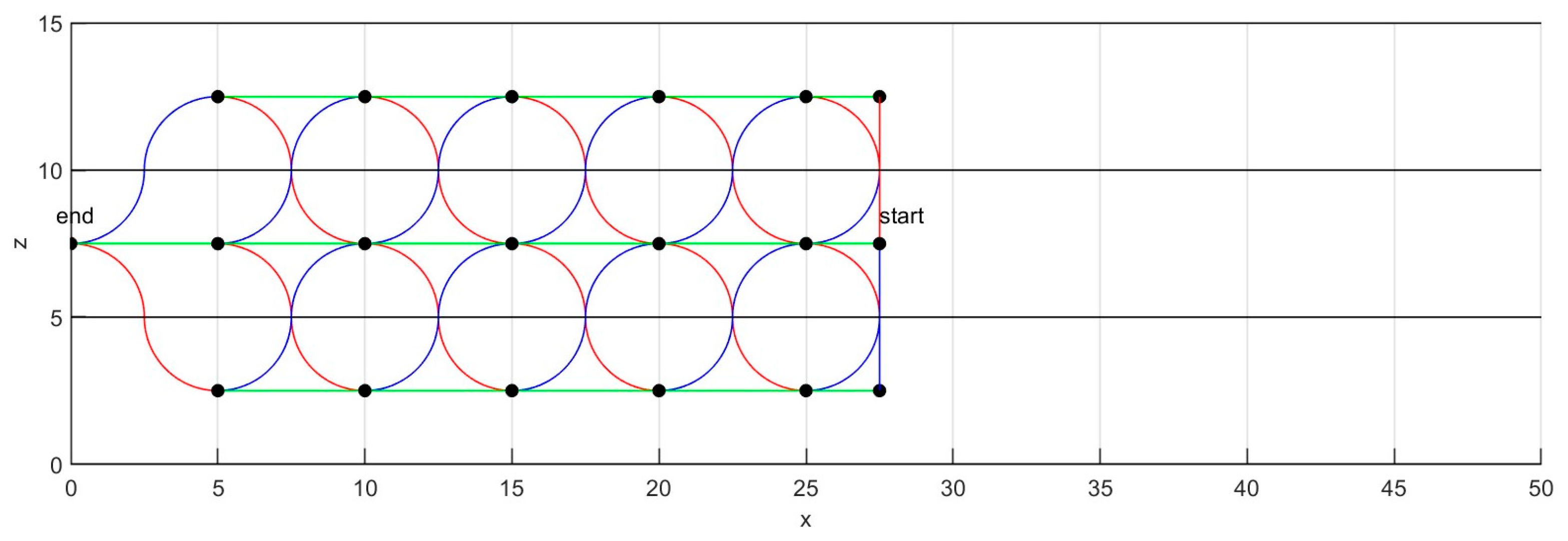
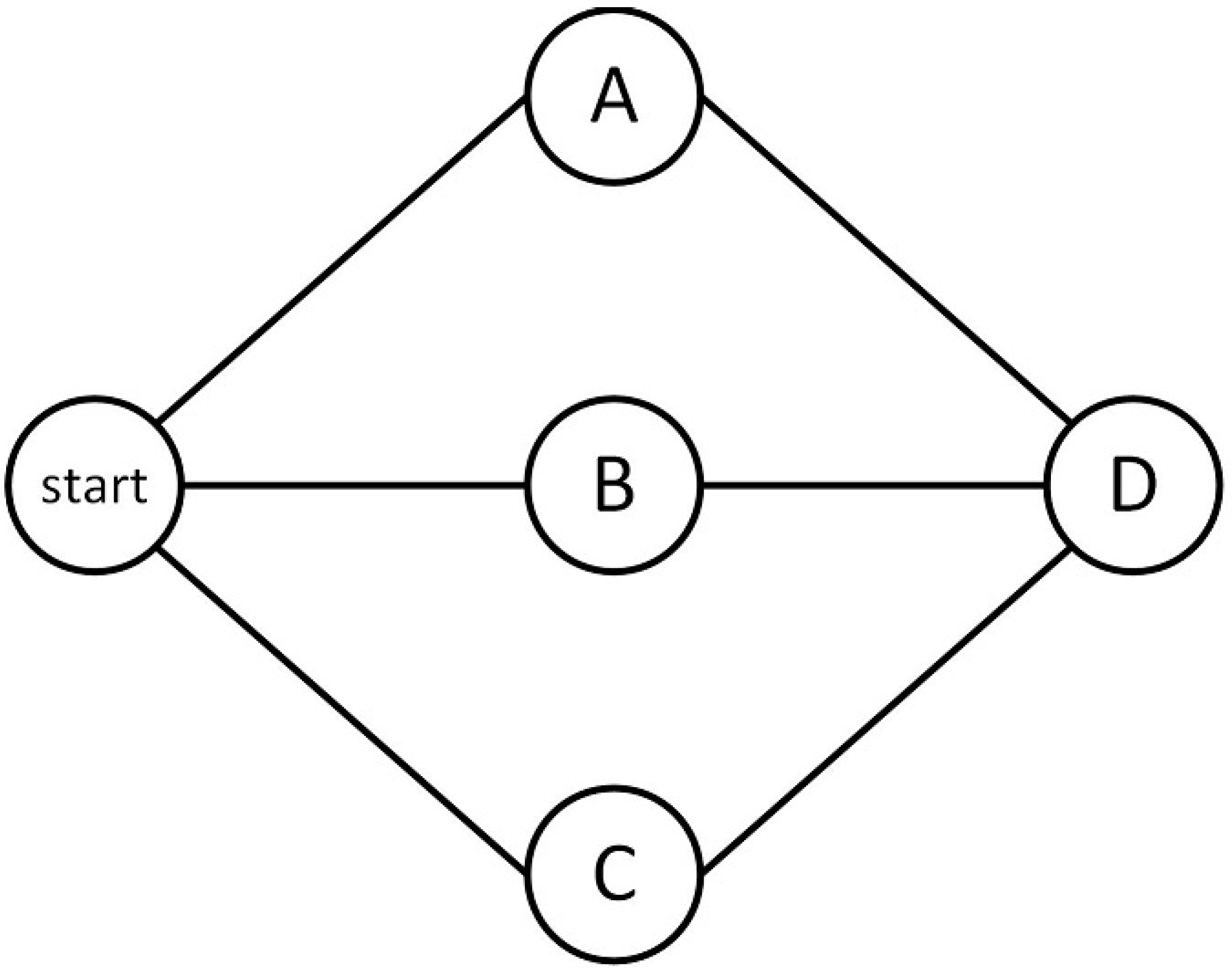
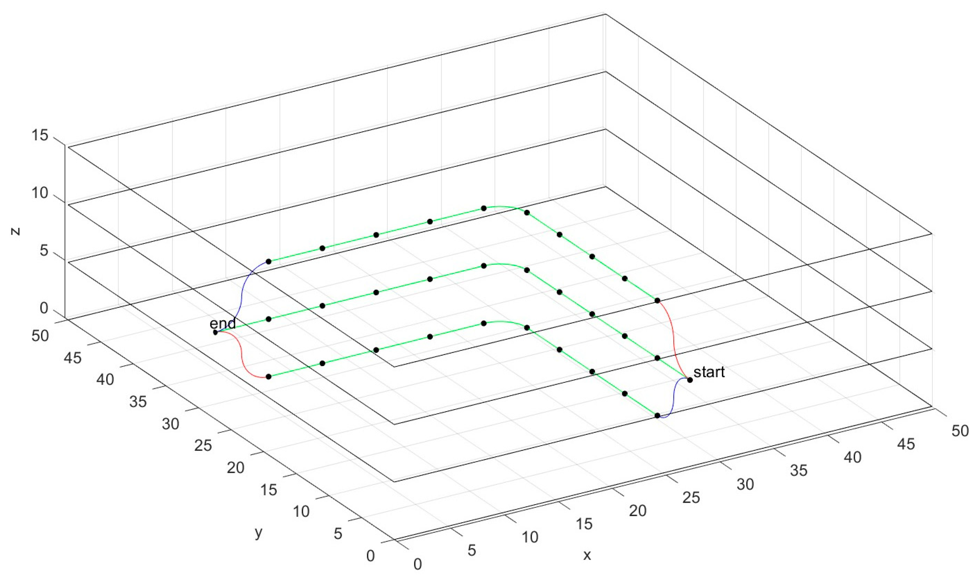
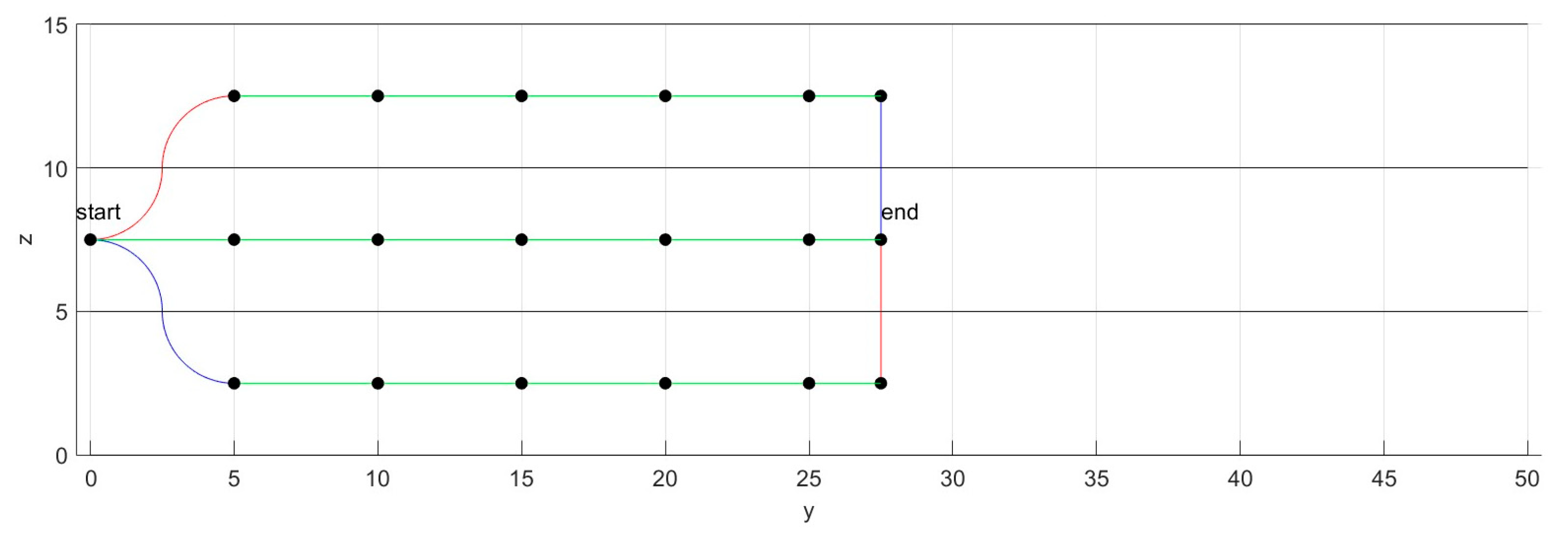
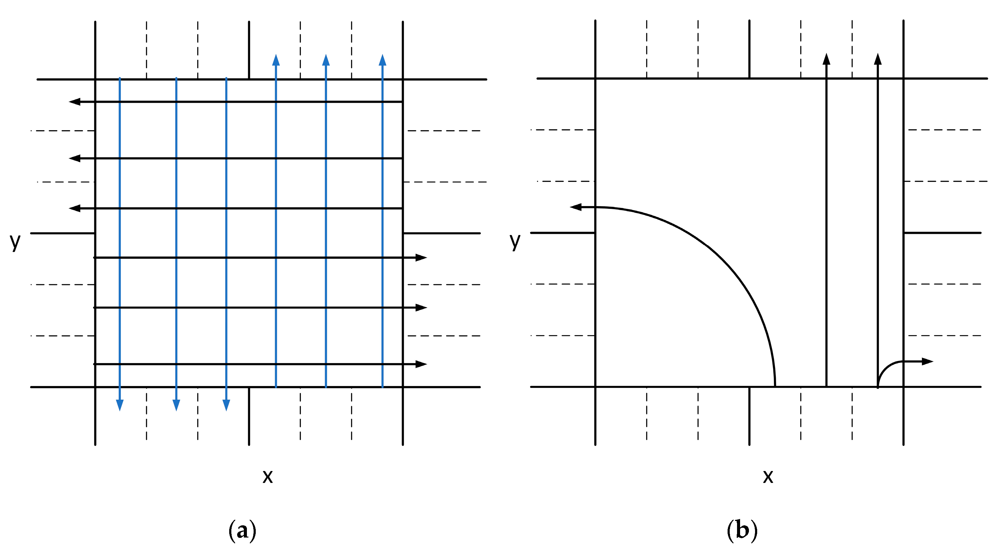
5. Paths of a UAV in the Intersection
6. Scheduling Scheme
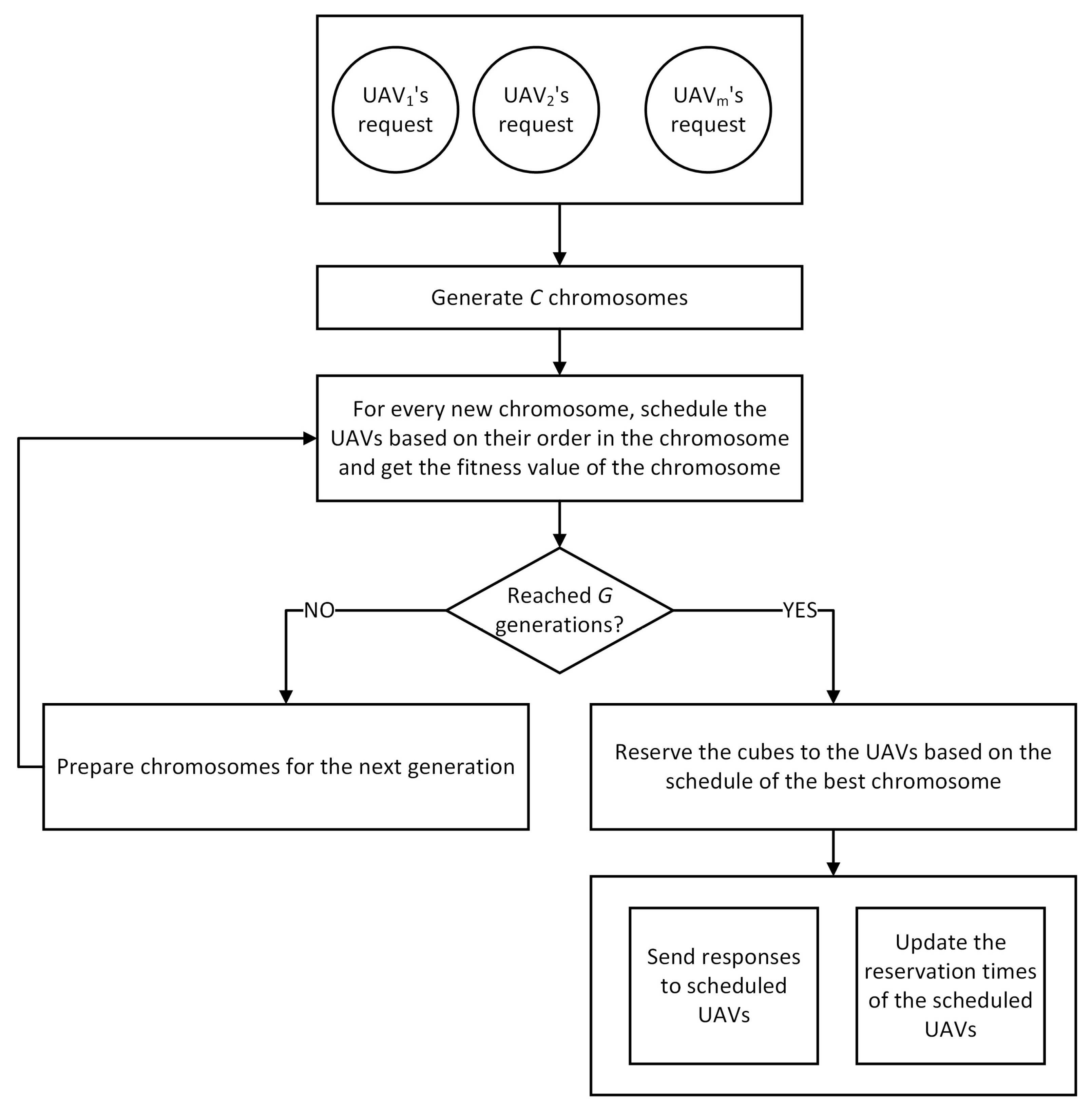
6.1. Using Genetic Algorithm to Decide the Scheduling Sequence
6.2. Tasks of the Intersection Manager
6.3. Scheduling a UAV
| Algorithm 1 Scheduling a UAV |
| Get |
| Set as empty set |
| Set as null |
| while is null or < |
| if is null or ’s exit time < P’s exit time then |
| end if |
| end while |
| reserve the cubes the UAV will occupy in |
- Finding the fastest path in the intersection: findfastestpath
| Algorithm 2 Finding the fastest path from start node to end node given the UAV will enter the intersection at |
| findfastestpath(, UAV’s size, UAV’s lane) |
| while is not emtpy |
| set as node from open list with minimum |
| remove from |
| for each ’s successor |
| , , , |
| if is true then |
| length of the path from to |
| manhattan distance from to end node |
| set as parent of |
| if is end node then stop search |
| else add to open list |
| end if |
| end if |
| end for |
| end while |
| if end node is reached then |
| get path from start node to end node |
| return |
| end if |
- Checking the path between nodes: checkPathToSuccessor
| Algorithm 3 Checking if the cubes the UAV will occupy from to do not conflict with other reservations |
| checkPathToSuccessor, , , ) compute compute true for each cube of = ’s Red-Black Tree node = root of while and is true if then else if then else false end if end while if is false then break the for loop end if end for return |
- Determining the cubes a UAV will occupy between nodes
| Algorithm 4 Simulation to determine the cubes a UAV will occupy when it travels from to |
| getCubesToOccupy(, ) initialize as empty set initialize as empty set initialize as empty set set simulation iteration while if is equal to 1 then else end if position the UAV at while UAV has not yet reached move UAV by get the cubes that UAV occupies at current position for each cube it occupies if cube is not in then insert cube to insert to insert to else set of cube to end if end for end while = i + 1 end while store , , |
7. Discussion of the Scheduling Algorithm
7.1. Complexity of the Scheduling Algorithm
7.2. Reducing the Complexity of the Scheduling Algorithm
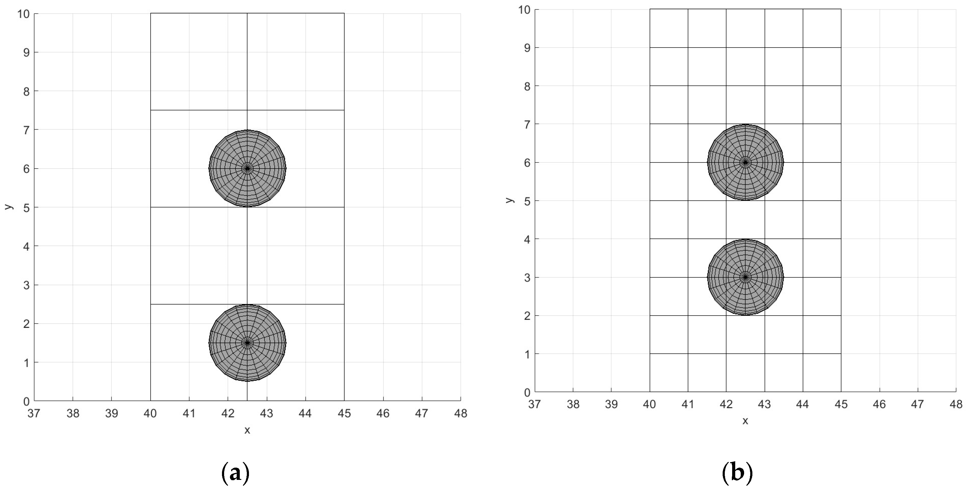
7.3. Effect of the Cube Size to the Efficiency in the Intersection
8. Simulation Results
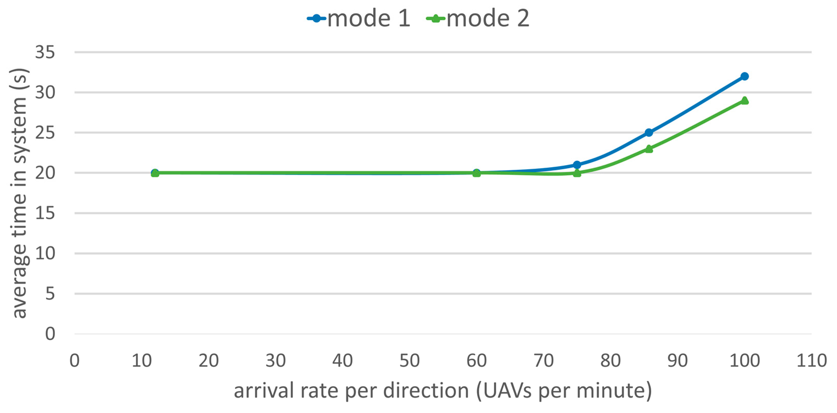
8.1. Performance of the System in Mode 1 and Mode 2
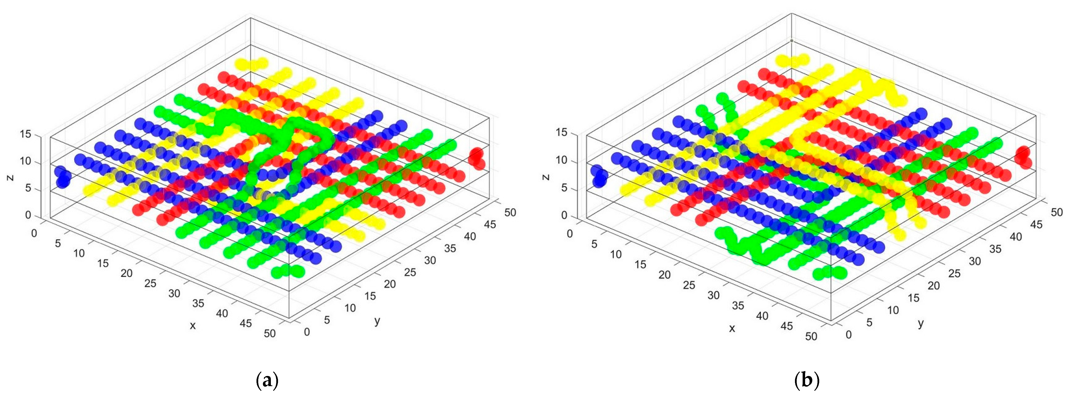
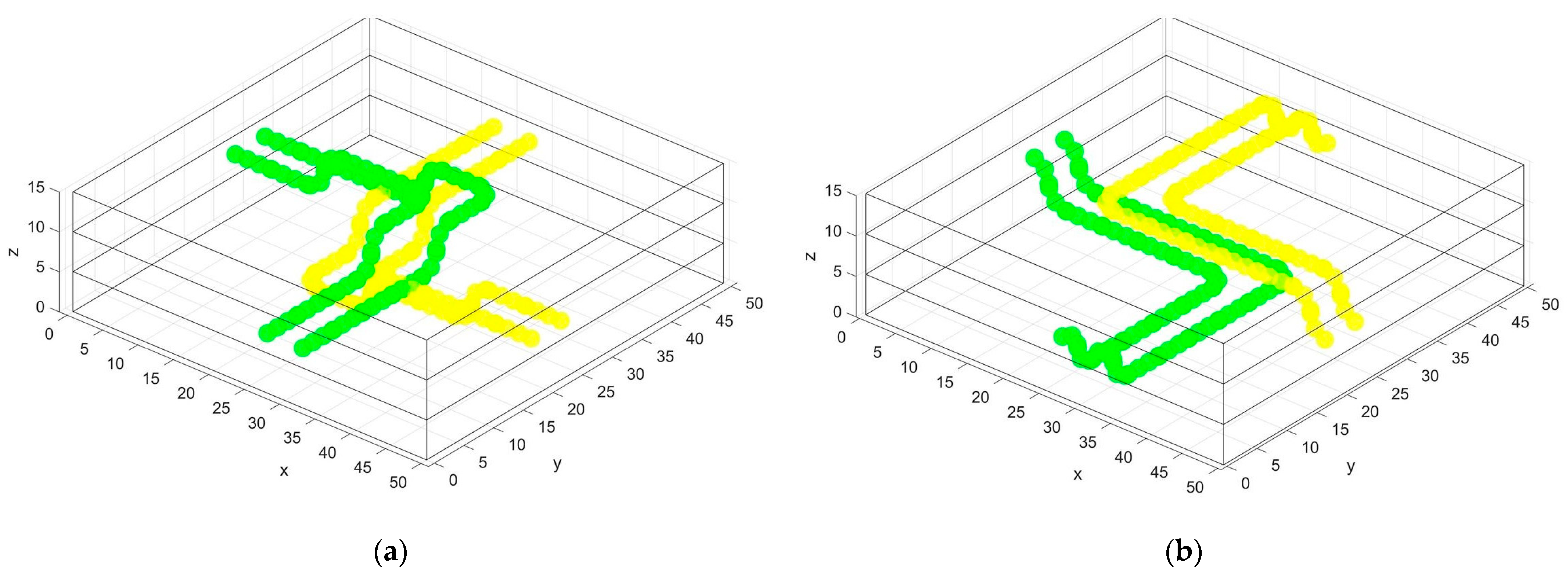
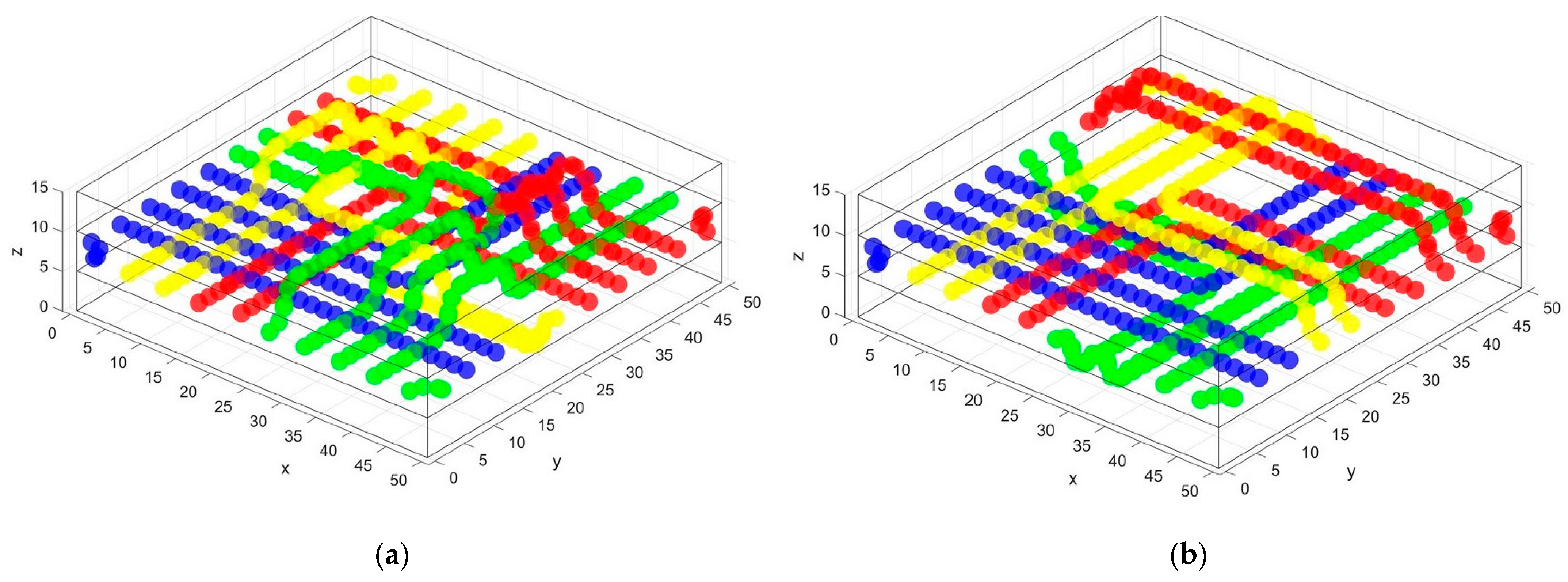
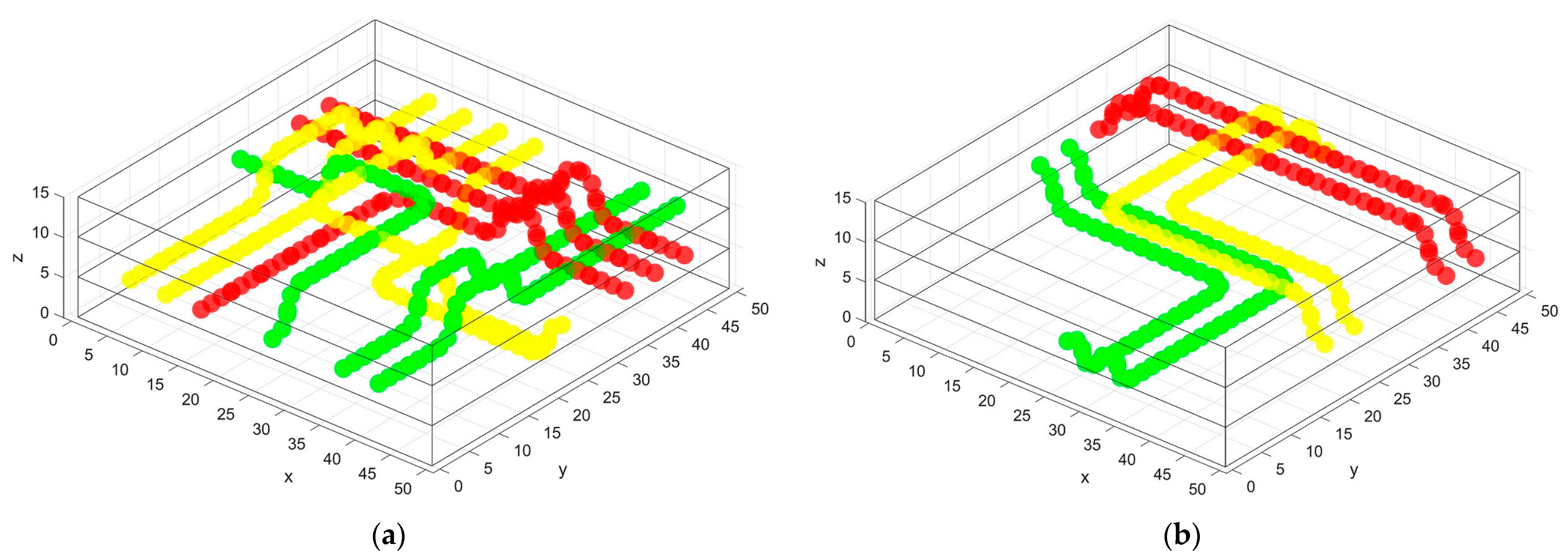
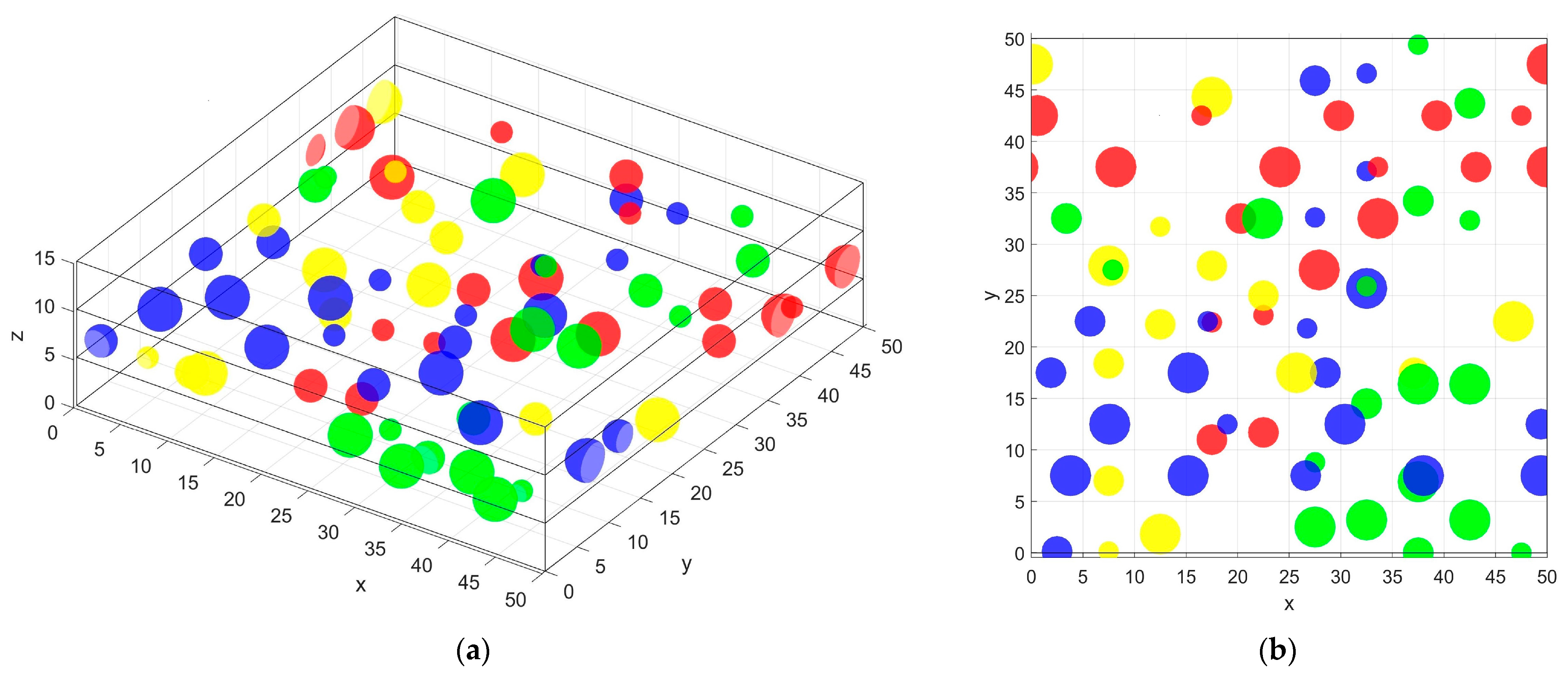
8.2. Sample Trajectories of UAVs
8.3. Evaluation of the Scheduling Sequence
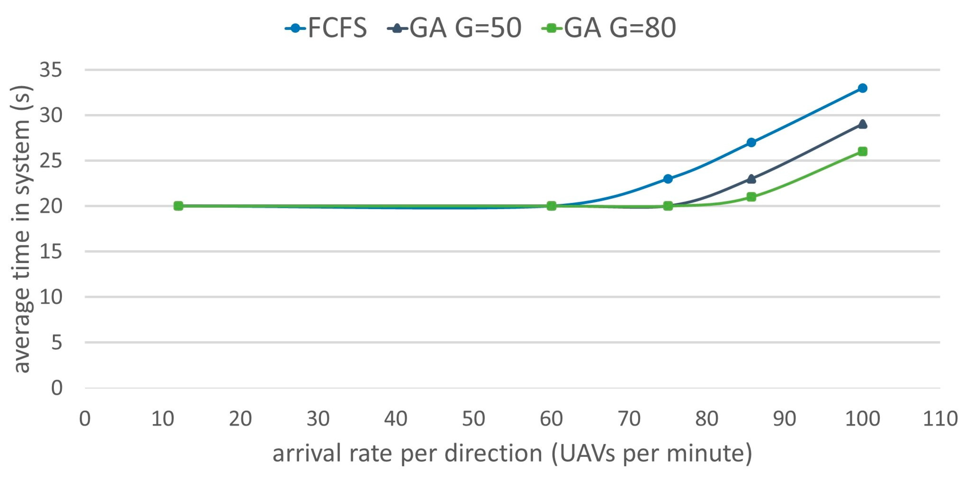
8.3.1. Comparison of our Proposed System with FCFS Scheduling
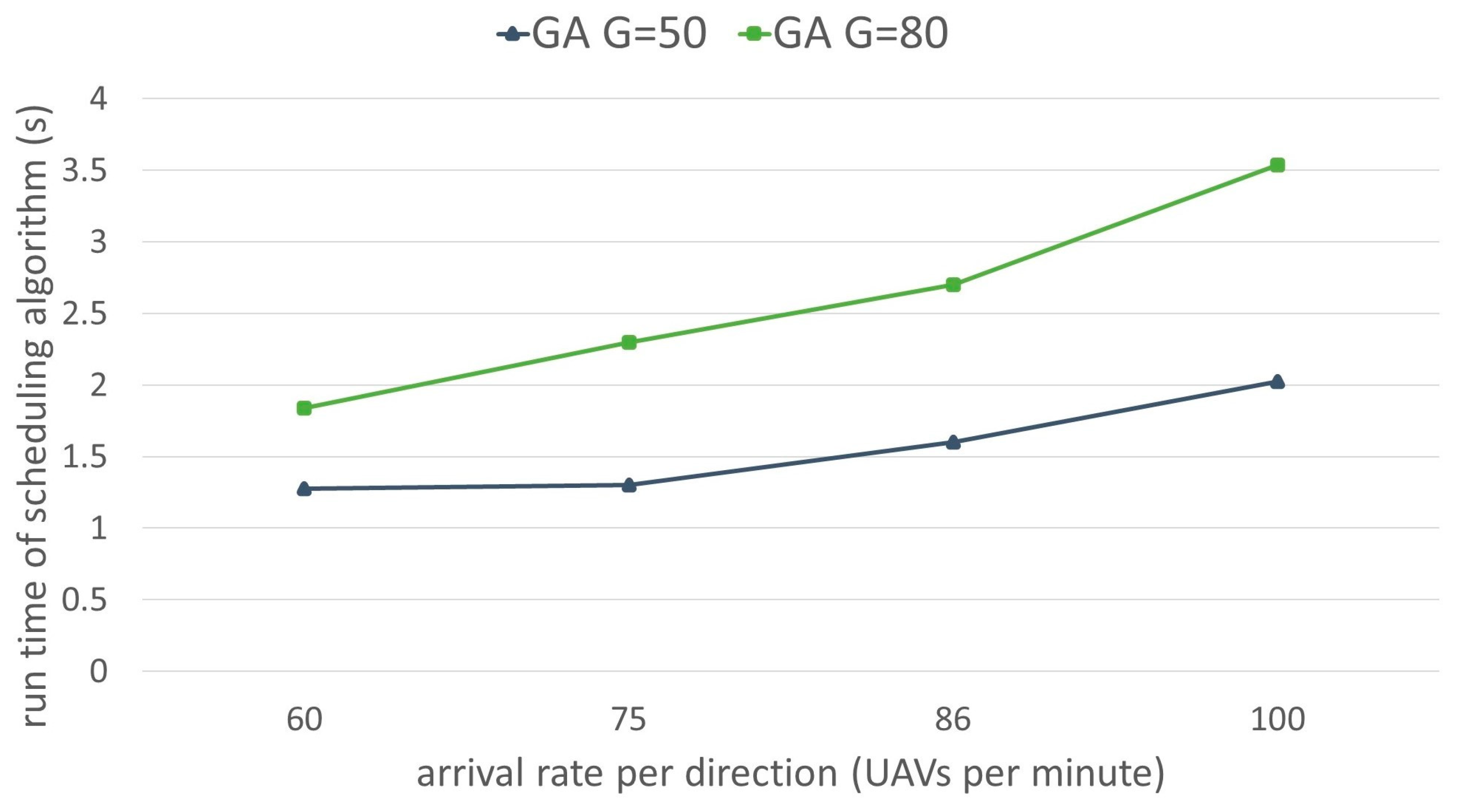
8.3.2. Run Time of the Scheduling Algorithm
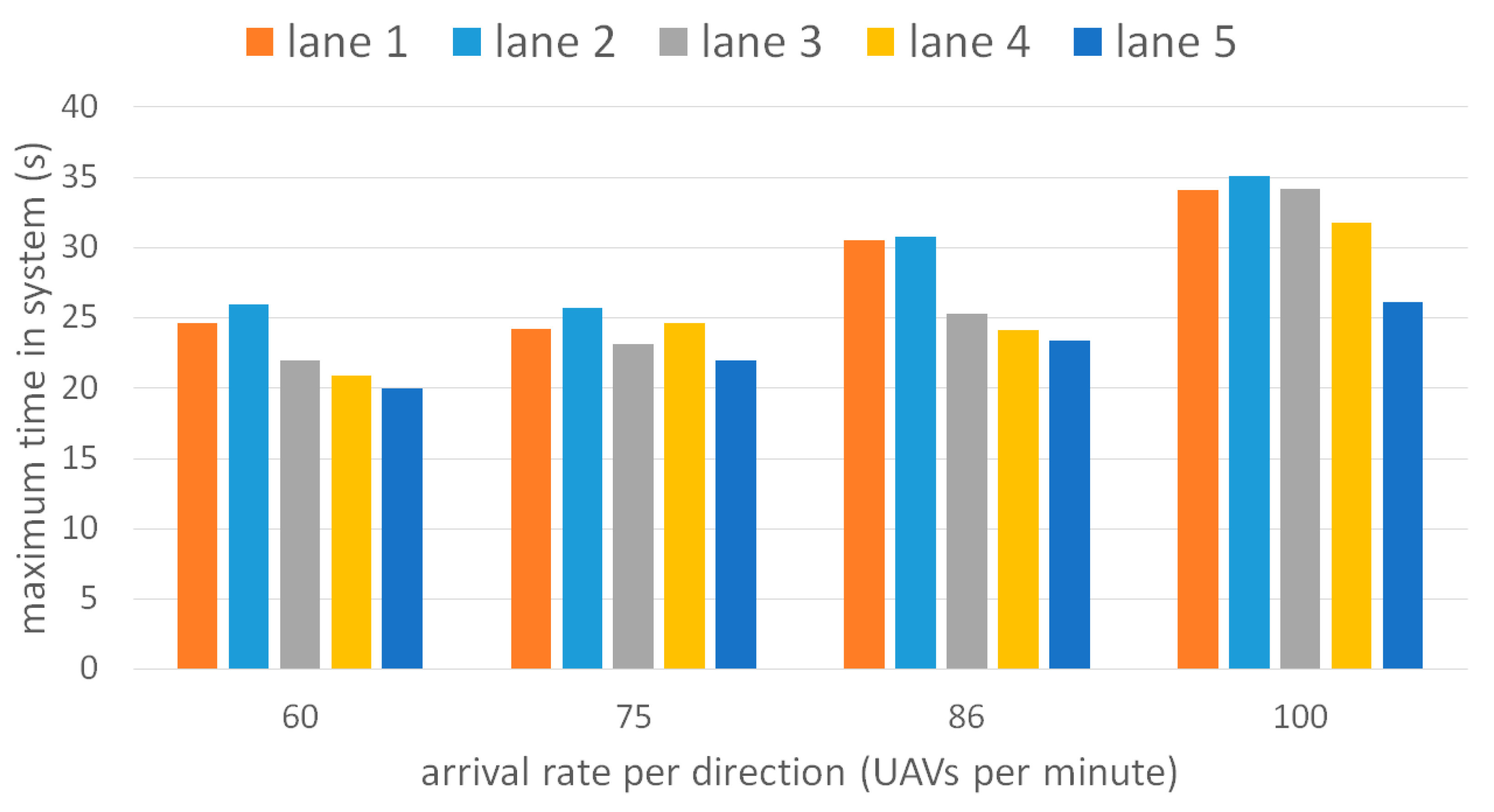
8.3.3. Maximum Time Spent per Lane of the UAVs
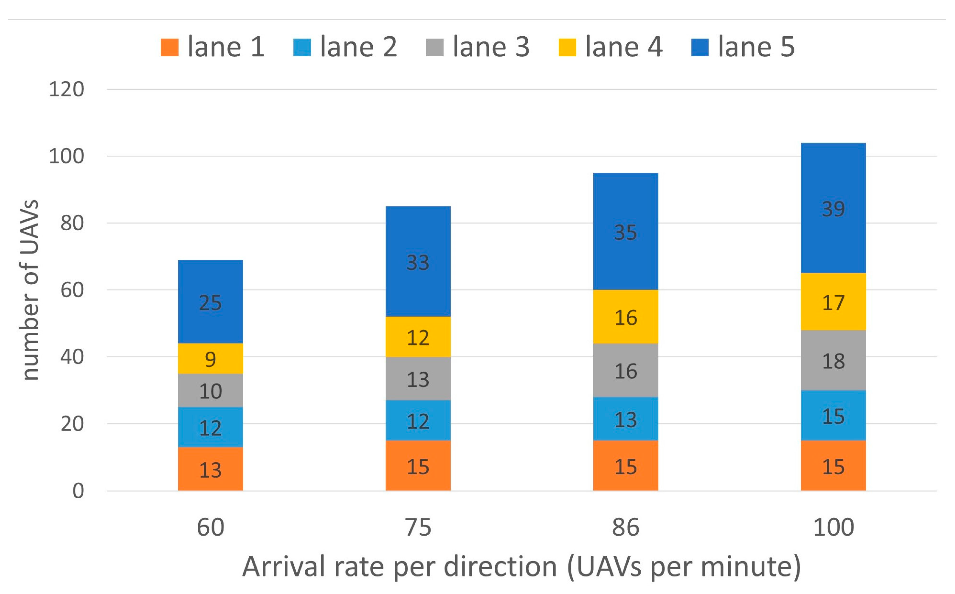
8.3.4. Number of UAVs That Crossed the Intersection per Lane
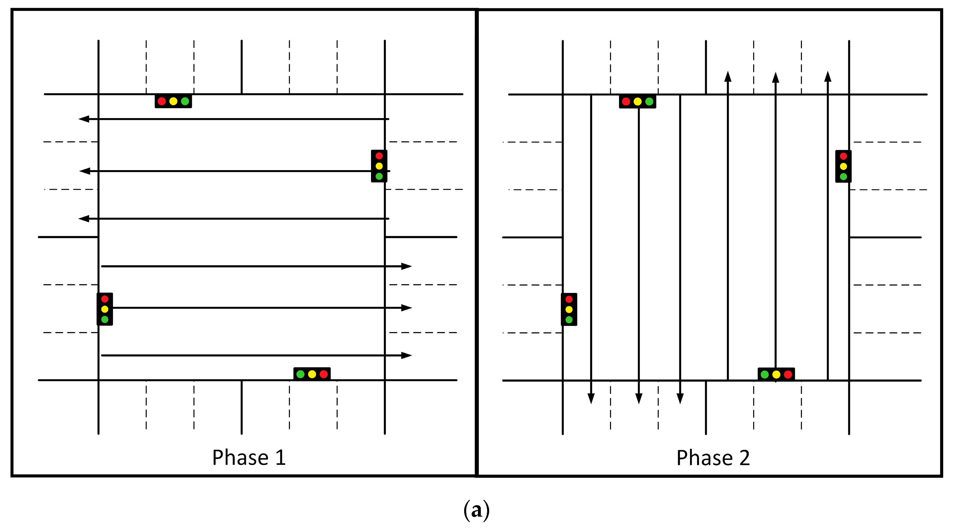
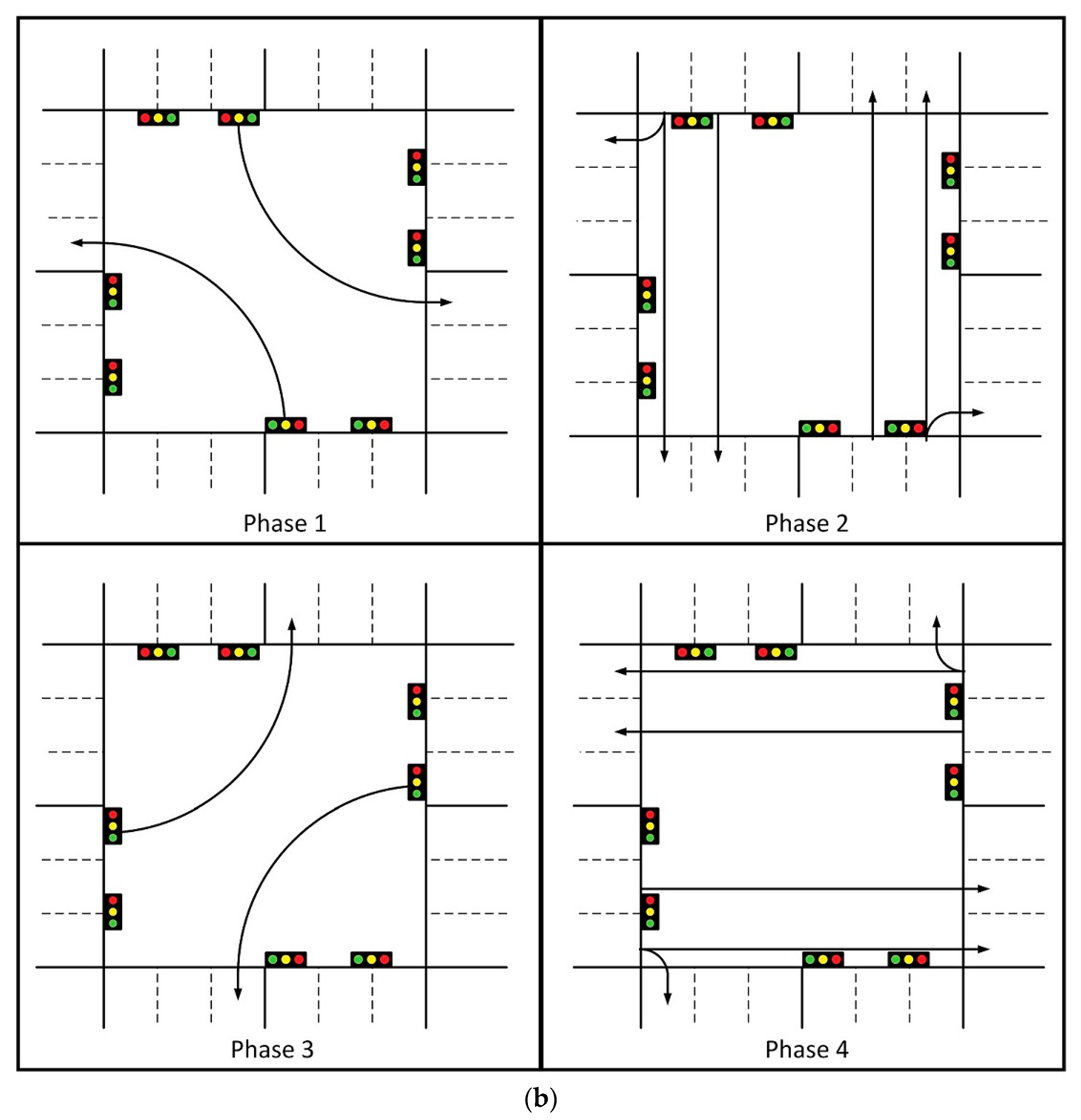
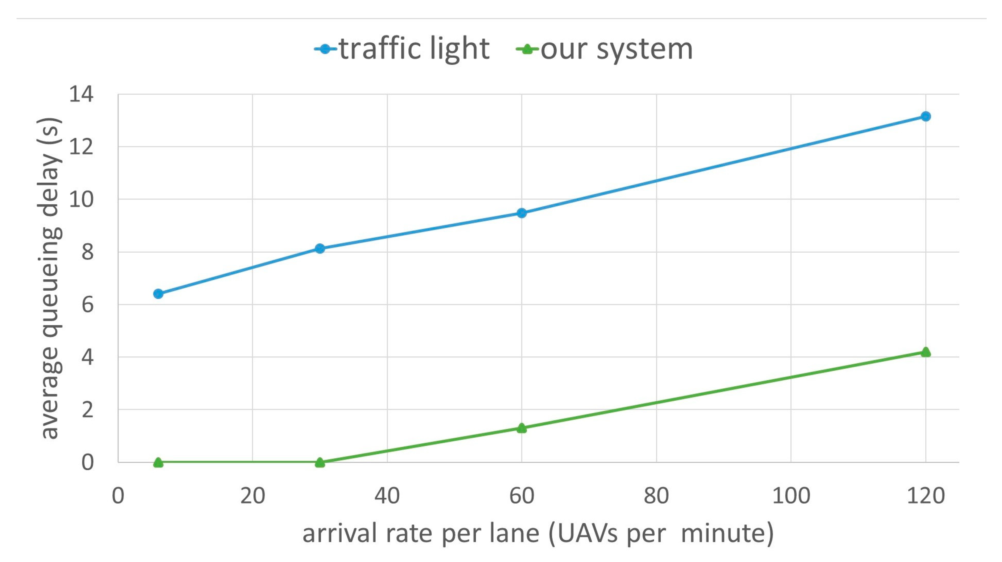
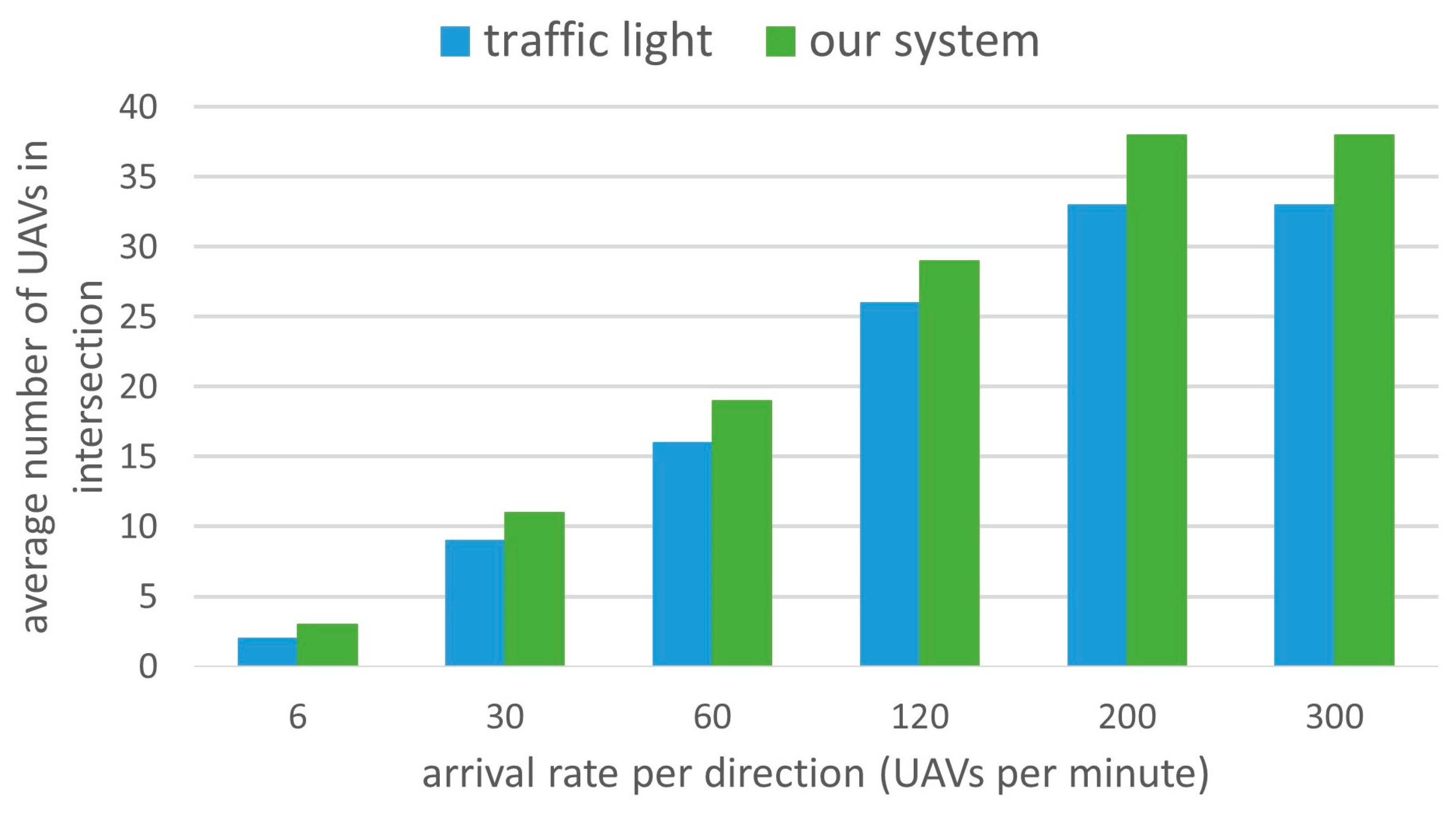
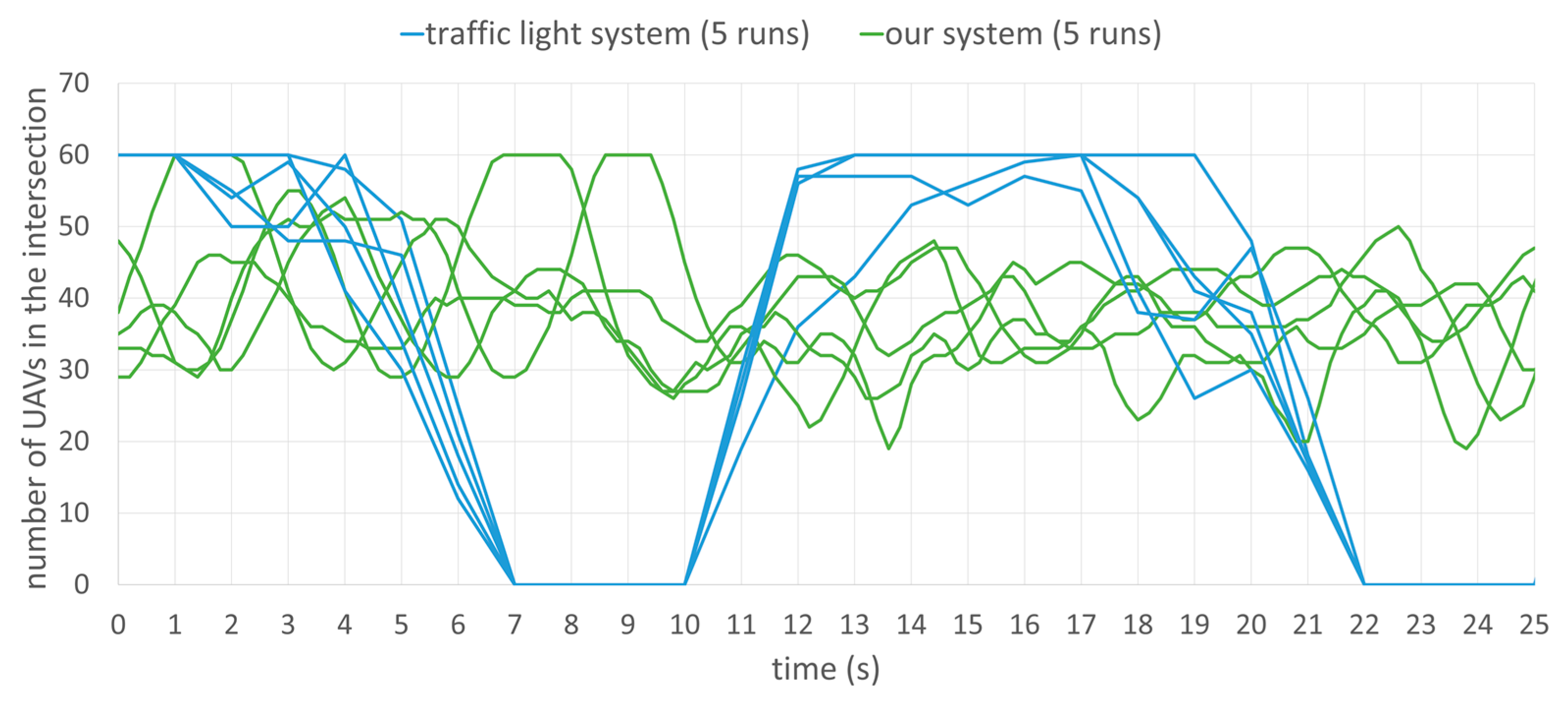
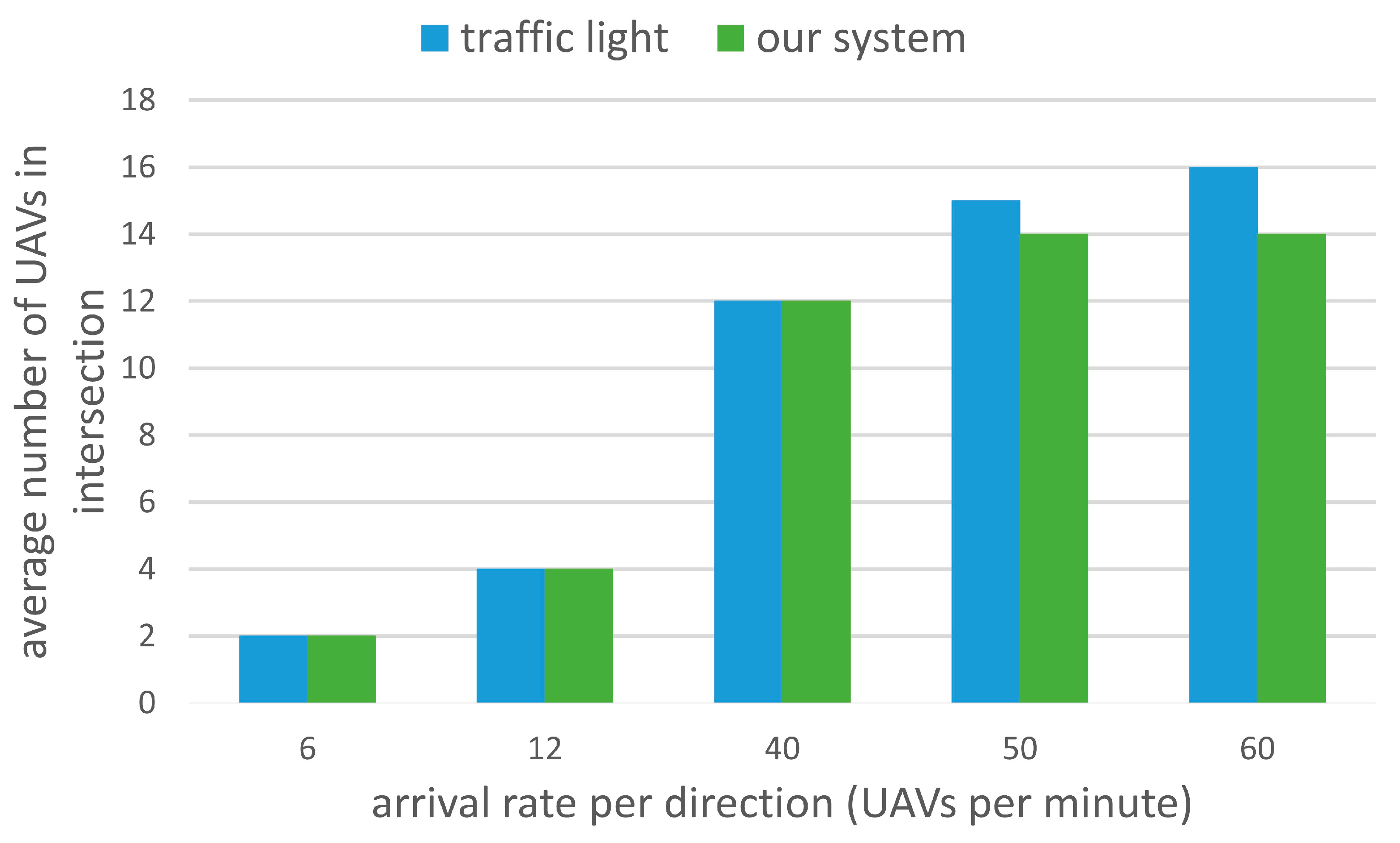
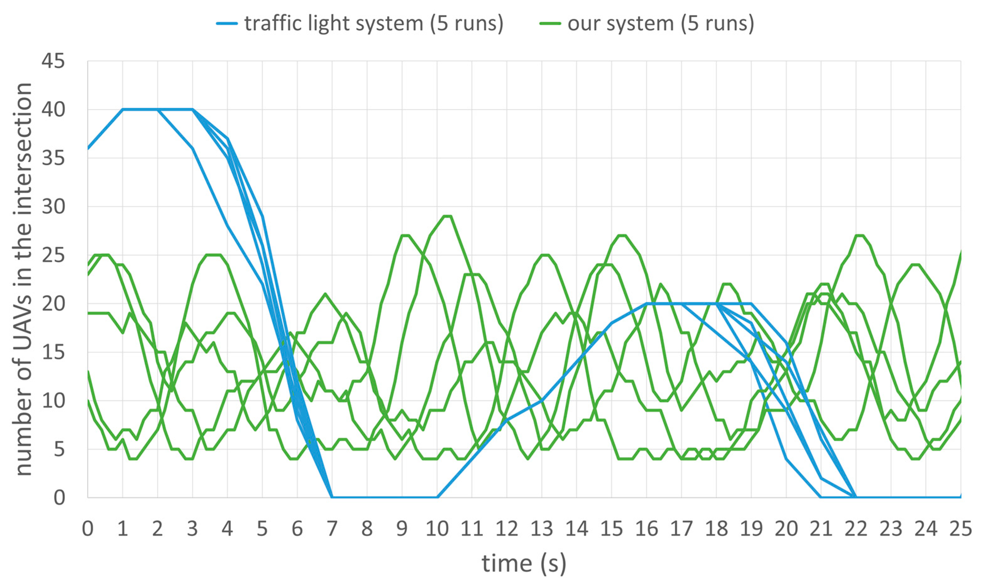
8.4. Comparison of Our Proposed System with the 2D Optimal Static Traffic Light Intersection System
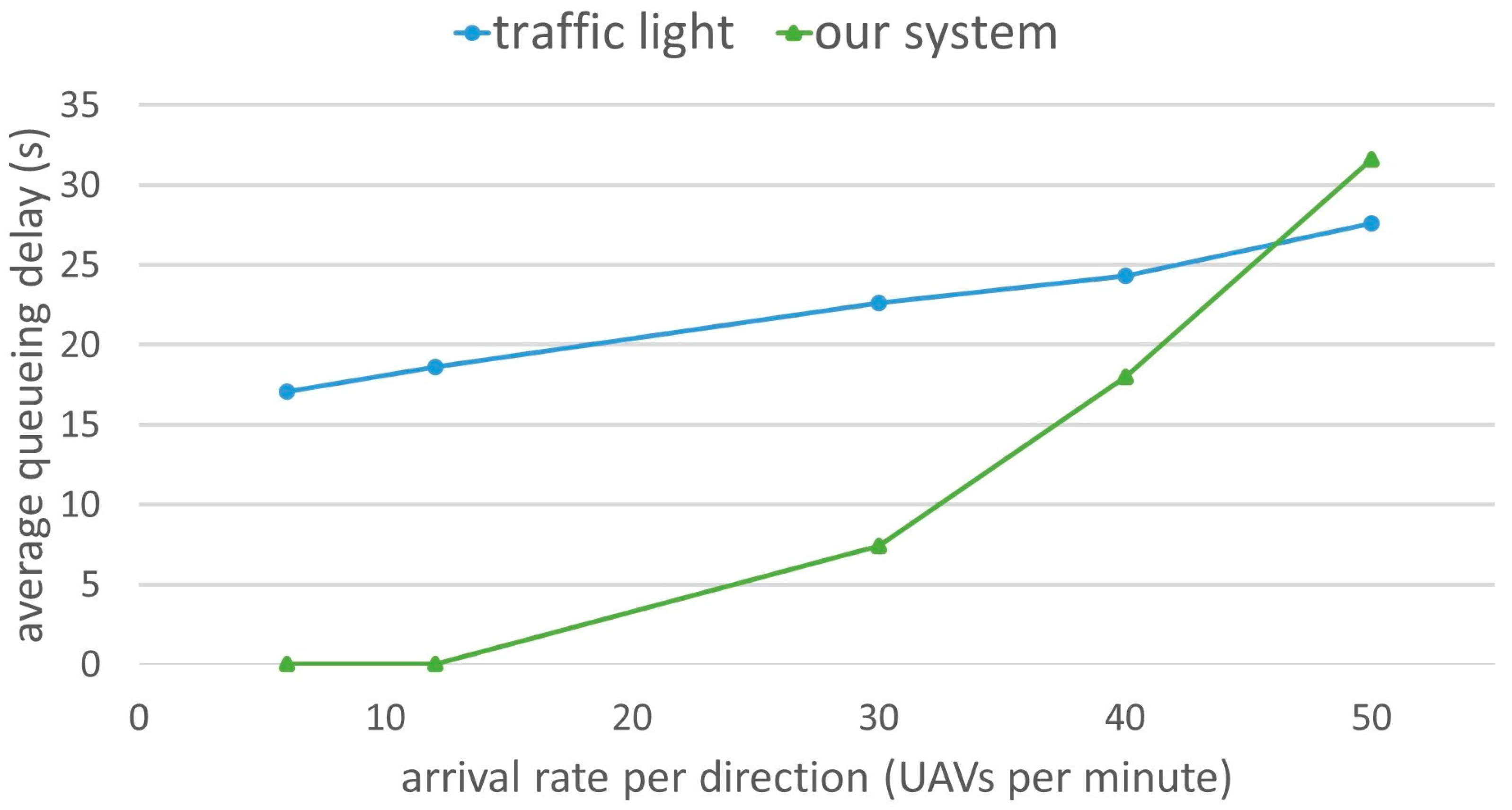
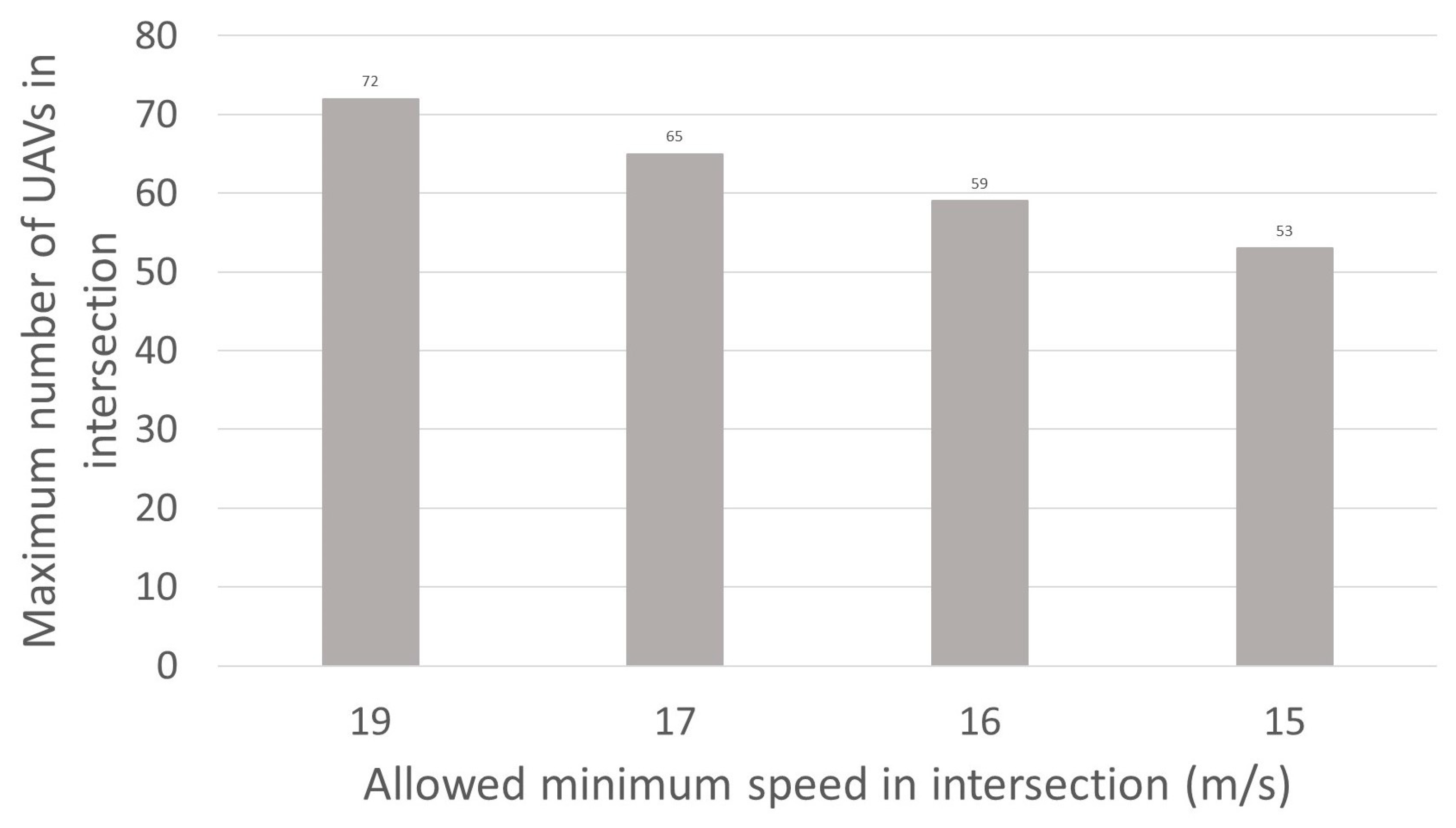
8.5. Efficiency of Our System on Different Values of the Allowed Speed Range in the Intersection
9. Conclusions
Author Contributions
Funding
Conflicts of Interest
References
- Balamurugan, N.M.; Mohan, S.; Adimoolam, M.; John, A.; Wang, W. DOA tracking for seamless connectivity in beamformed IoT-based drones. Comput. Stand. Interfaces 2021, 79, 103564. [Google Scholar] [CrossRef]
- Cai, Y.; Cui, F.; Shi, Q.; Zhao, M.; Li, G.Y. Dual-UAV-enabled secure communications: Joint trajectory design and user scheduling. IEEE J. Sel. Areas Commun. 2018, 36, 1972–1985. [Google Scholar] [CrossRef]
- Kopardekar, P.; Rios, J.; Prevot, T.; Johnson, M.; Jung, J.; Robinson, J.E. Unmanned aircraft system traffic management (UTM) concept of operations. In Proceedings of the AIAA Aviation and Aeronautics Forum, Washington, DC, USA, 13 June 2016. [Google Scholar]
- Xu, C.; Liao, X.; Tan, J.; Ye, H.; Lu, H. Recent research progress of unmanned aerial vehicle regulation policies and technologies in urban low altitude. IEEE Access 2020, 8, 74175–74194. [Google Scholar] [CrossRef]
- Dresner, K.; Stone, P. Multiagent traffic management: A reservation-based intersection control mechanism. In Proceedings of the Third International Joint Conference on Autonomous Agents and Multiagent Systems, New York, NY, USA, 23 July 2004; pp. 530–537. [Google Scholar]
- Kuru, K. Planning the Future of Smart Cities with Swarms of Fully Autonomous Unmanned Aerial Vehicles Using a Novel Framework. IEEE Access 2021, 9, 6571–6595. [Google Scholar] [CrossRef]
- Ho, F.; Geraldes, R.; Gonçalves, A.; Rigault, B.; Sportich, B.; Kubo, D.; Cavazza, M.; Prendinger, H. Decentralized multi-agent path finding for UAV traffic management. IEEE Trans. Intell. Transp. Syst. 2020, in press. [Google Scholar] [CrossRef]
- Labib, N.S.; Danoy, G.; Musial, J.; Brust, M.R.; Bouvry, P. A multilayer low-altitude airspace model for UAV traffic management. In Proceedings of the 9th ACM Symposium on Design and Analysis of Intelligent Vehicular Networks and Applications, Miami, FL, USA, 25–29 November 2019; pp. 57–63. [Google Scholar]
- Labib, N.S.; Danoy, G.; Musial, J.; Brust, M.R.; Bouvry, P. Internet of unmanned aerial vehicles—A multilayer low-altitude airspace model for distributed UAV traffic management. Sensors 2019, 19, 4779. [Google Scholar] [CrossRef] [PubMed] [Green Version]
- Yasin, J.N.; Mohamed, S.A.; Haghbayan, M.H.; Heikkonen, J.; Tenhunen, H.; Plosila, J. Unmanned aerial vehicles (uavs): Collision avoidance systems and approaches. IEEE Access 2020, 8, 105139–105155. [Google Scholar] [CrossRef]
- Yang, L.; Qi, J.; Xiao, J.; Yong, X. A literature review of UAV 3D path planning. In Proceedings of the 11th World Congress on Intelligent Control and Automation, Shenyang, China, 29 June 2014; pp. 2376–2381. [Google Scholar]
- Lin, Y.; Saripalli, S. Sampling-based path planning for UAV collision avoidance. IEEE Trans. Intell. Transp. Syst. 2017, 18, 3179–3192. [Google Scholar] [CrossRef]
- Lin, Y.; Saripalli, S. Path planning using 3D dubins curve for unmanned aerial vehicles. In Proceedings of the IEEE International Conference on Unmanned Aircraft Systems (ICUAS), Orlando, FL, USA, 27–10 May 2014; pp. 296–304. [Google Scholar]
- Hrabar, S. 3D path planning and stereo-based obstacle avoidance for rotorcraft UAVs. In Proceedings of the IEEE/RSJ International Conference on Intelligent Robots and Systems, Nice, France, 22 September 2008; pp. 807–814. [Google Scholar]
- Yan, F.; Liu, Y.S.; Xiao, J.Z. Path planning in complex 3D environments using a probabilistic roadmap method. Int. J. Control Autom. 2013, 10, 525–533. [Google Scholar] [CrossRef]
- Eun, Y.; Bang, H. Cooperative task assignment and path planning of multiple UAVs using genetic algorithm. In Proceedings of the AIAA Infotech at Aerospace 2007 Conference and Exhibit, Rohnert Park, CA, USA, 7–10 May 2007; p. 2982. [Google Scholar]
- Lugo-Cárdenas, I.; Flores, G.; Salazar, S.; Lozano, R. Dubins path generation for a fixed wing UAV. In Proceedings of the International conference on unmanned aircraft systems (ICUAS), Orlando, FL, USA, 27 May 2014; pp. 339–346. [Google Scholar]
- Yan, P.; Yan, Z.; Zheng, H.; Guo, J. A Fixed Wing UAV Path Planning Algorithm Based On Genetic Algorithm and Dubins Curve Theory. In Proceedings of the International Conference on Mechanical, Material and Aerospace Engineering, Wuhan, China, 10–13 May 2018. [Google Scholar]
- Yan, F.; Zhu, X.; Zhou, Z.; Chu, J. A hierarchical mission planning method for simultaneous arrival of multi-UAV coalition. Appl. Sci. 2019, 9, 1986. [Google Scholar] [CrossRef] [Green Version]
- Shah, M.A.; Aouf, N. 3D cooperative Pythagorean hodograph path planning and obstacle avoidance for multiple UAVs. In Proceedings of the IEEE 9th International Conference on Cybernetic Intelligent Systems, Reading, UK, 1 September 2010; pp. 1–6. [Google Scholar]
- Nabi-Abdolyousefi, R.; Banazadeh, A. 3D offline path planning for a surveillance aerial vehicle using B-splines. In Proceedings of the International Conference on Advanced Mechatronic Systems, Luoyang, China, 25 September 2013; pp. 306–311. [Google Scholar]
- Mittal, S.; Deb, K. Three-dimensional offline path planning for UAVs using multiobjective evolutionary algorithms. In Proceedings of the IEEE Congress on Evolutionary Computation, Singapore, 25 September 2007; pp. 3195–3202. [Google Scholar]
- Nikolos, I.K.; Valavanis, K.P.; Tsourveloudis, N.C.; Kostaras, A.N. Evolutionary algorithm based offline/online path planner for UAV navigation. IEEE Trans. Syst. Man Cybern. B 2003, 33, 898–912. [Google Scholar] [CrossRef] [PubMed] [Green Version]
- Zhang, X.; Chen, J.; Xin, B.; Fang, H. Online path planning for UAV using an improved differential evolution algorithm. IFAC Proc. Vol. 2011, 44, 6349–6354. [Google Scholar] [CrossRef]
- Macharet, D.G.; Neto, A.A.; Campos, M.F. Feasible UAV path planning using genetic algorithms and Bézier curves. In Proceedings of the Brazilian Symposium on Artificial Intelligence, São Bernardo do Campo, Brazil, 23 October 2010; pp. 223–232. [Google Scholar]
- Sathyaraj, B.M.; Jain, L.C.; Finn, A.; Drake, S. Multiple UAVs path planning algorithms: A comparative study. Fuzzy Optim. Decis. Mak. 2008, 7, 257–267. [Google Scholar] [CrossRef]
- Meng, B.B.; Gao, X. UAV path planning based on bidirectional sparse A* search algorithm. In Proceedings of the International Conference on Intelligent Computation Technology and Automation, Changsha, China, 11 May 2010; pp. 1106–1109. [Google Scholar]
- Zhan, W.; Wang, W.; Chen, N.; Wang, C. Efficient UAV path planning with multiconstraints in a 3D large battlefield environment. Math. Probl. Eng. 2014, 2014, 12. [Google Scholar] [CrossRef]
- Koenig, S.; Likhachev, M. Fast replanning for navigation in unknown terrain. IEEE Trans. Robot. 2005, 21, 354–363. [Google Scholar] [CrossRef]
- Shim, D.H.; Sastry, S. An evasive maneuvering algorithm for UAVs in see-and-avoid situations. In Proceedings of the IEEE American Control Conference, New York, NY, USA, 9–14 July 2007; pp. 3886–3891. [Google Scholar]
- Ho, F.; Geraldes, R.; Goncalves, A.; Cavazza, M.; Prendinger, H. Improved conflict detection and resolution for service UAVs in shared airspace. IEEE Trans. Veh. Technol. 2018, 68, 1231–1242. [Google Scholar] [CrossRef]
- Radmanesh, M.; Kumar, M. Flight formation of UAVs in presence of moving obstacles using fast-dynamic mixed integer linear programming. Aerosp. Sci. Technol. 2016, 50, 149–160. [Google Scholar] [CrossRef] [Green Version]
- Selvam, P.K.; Raja, G.; Rajagopal, V.; Dev, K.; Knorr, S. Collision-free Path Planning for UAVs using Efficient Artificial Potential Field Algorithm. In Proceedings of the IEEE 93rd Vehicular Technology Conference (VTC2021-Spring), Helsinki, Finland, 25–28 April 2021. [Google Scholar]
- Hrabar, S. Reactive obstacle avoidance for rotorcraft uavs. In Proceeding of the IEEE/RSJ International Conference on Intelligent Robots and Systems, San Francisco, CA, USA, 25 September 2011; pp. 4967–4974. [Google Scholar]
- Sigurd, K.; How, J. UAV trajectory design using total field collision avoidance. In Proceedings of the AIAA Guidance, Navigation, and Control Conference and Exhibit, Austin, TX, USA, 11–14 August 2003; p. 5728. [Google Scholar]
- Ferrera, E.; Alcántara, A.; Capitán, J.; Castaño, A.R.; Marrón, P.J.; Ollero, A. Decentralized 3d collision avoidance for multiple uavs in outdoor environments. Sensors 2018, 18, 4101. [Google Scholar] [CrossRef] [Green Version]
- Choi, M.; Rubenecia, A.; Shon, T.; Choi, H.H. Velocity obstacle based 3d collision avoidance scheme for low-cost micro uavs. Sustainability 2017, 9, 1174. [Google Scholar] [CrossRef] [Green Version]
- Huang, S.; Teo, R.S.H.; Liu, W. Distributed Cooperative Avoidance Control for Multi-Unmanned Aerial Vehicles. Actuators 2019, 8, 1. [Google Scholar] [CrossRef] [Green Version]
- Albaker, B.M.; Rahim, N.A. Autonomous unmanned aircraft collision avoidance system based on geometric intersection. Phys. Sci. Int. J. 2011, 6, 391–401. [Google Scholar]
- Douthwaite, J.A.; De Freitas, A.; Mihaylova, L.S. An interval approach to multiple unmanned aerial vehicle collision avoidance. In Proceedings of the 2017 Sensor Data Fusion: Trends, Solutions, Applications (SDF), Bonn, Germany, 10–12 October 2017. [Google Scholar]
- Khosiawan, Y.; Park, Y.; Moon, I.; Nilakantan, J.M.; Nielsen, I. Task scheduling system for UAV operations in indoor environment. Neural. Comput. Appl. 2019, 31, 5431–5459. [Google Scholar] [CrossRef] [Green Version]
- Pérez-Carabaza, S.; Scherer, J.; Rinner, B.; López-Orozco, J.A.; Besada-Portas, E. UAV trajectory optimization for Minimum Time Search with communication constraints and collision avoidance. Eng. Appl. Artif. Intel. 2019, 85, 357–371. [Google Scholar] [CrossRef]
- Yang, Q.; Yoo, S.J. Optimal UAV path planning: Sensing data acquisition over IoT sensor networks using multi-objective bio-inspired algorithms. IEEE Access 2018, 6, 13671–13684. [Google Scholar] [CrossRef]
- Bayrak, A.; Efe, M.Ö. FPGA based offline 3D UAV local path planner using evolutionary algorithms for unknown environments. In Proceedings of the Annual Conference of the IEEE Industrial Electronics Society, Florence, Italy, 23 October 2016; pp. 4778–4783. [Google Scholar]
- Hayat, S.; Yanmaz, E.; Bettstetter, C.; Brown, T.X. Multi-objective drone path planning for search and rescue with quality-of-service requirements. Auton Robot. 2020, 44, 1183–1198. [Google Scholar] [CrossRef]
- Wan, X.; Ghazzai, H.; Massoud, Y.; Menouar, H. Optimal collision-free navigation for multi-rotor UAV swarms in urban areas. In Proceedings of the 2019 IEEE 89th Vehicular Technology Conference (VTC2019-Spring), Kuala Lumpur, Malaysia, 28 April–1 May 2019. [Google Scholar]
- Bahabry, A.; Wan, X.; Ghazzai, H.; Menouar, H.; Vesonder, G.; Massoud, Y. Low-altitude navigation for multi-rotor drones in urban areas. IEEE Access 2019, 7, 87716–87731. [Google Scholar] [CrossRef]
- Bahabry, A.; Wan, X.; Ghazzai, H.; Vesonder, G.; Massoud, Y. Collision-free navigation and efficient scheduling for fleet of multi-rotor drones in smart city. In Proceedings of the 2019 IEEE 62nd International Midwest Symposium on Circuits and Systems (MWSCAS), Dallas, TX, USA, 4–7 August 2019; pp. 552–555. [Google Scholar]
- Suresh, P.; Saravanakumar, U.; Iwendi, C.; Mohan, S.; Srivastava, G. Field-programmable gate arrays in a low power vision system. Comput. Electr. Eng. 2021, 90, 106996. [Google Scholar]
- Shakhatreh, H.; Sawalmeh, A.H.; Al-Fuqaha, A.; Dou, Z.; Almaita, E.; Khalil, I.; Othman, N.S.; Khreishah, A.; Guizani, M. Unmanned aerial vehicles (UAVs): A survey on civil applications and key research challenges. IEEE Access 2019, 7, 48572–48634. [Google Scholar] [CrossRef]
- Chen, X.; Tang, J.; Lao, S. Review of Unmanned Aerial Vehicle Swarm Communication Architectures and Routing Protocols. Appl. Sci. 2020, 10, 3661. [Google Scholar] [CrossRef]
- Shiri, H.; Park, J.; Bennis, M. Communication-efficient massive UAV online path control: Federated learning meets mean-field game theory. arXiv 2020, arXiv:2003.04451. [Google Scholar] [CrossRef]
- He, L.; Bai, P.; Liang, X.; Zhang, J.; Wang, W. Feedback formation control of UAV swarm with multiple implicit leaders. Aerosp. Sci. Technol. 2018, 72, 327–334. [Google Scholar] [CrossRef]
- Bai, G.; Li, Y.; Fang, Y.; Zhang, Y.A.; Tao, J. Network approach for resilience evaluation of a UAV swarm by considering communication limits. Reliab. Eng. Syst. Saf. 2020, 193, 106602. [Google Scholar] [CrossRef]
- Mozaffari, M.; Saad, W.; Bennis, M.; Nam, Y.H.; Debbah, M. A tutorial on UAVs for wireless networks: Applications, challenges, and open problems. IEEE Commun. Surv. Tutor. 2019, 21, 2334–2360. [Google Scholar] [CrossRef] [Green Version]
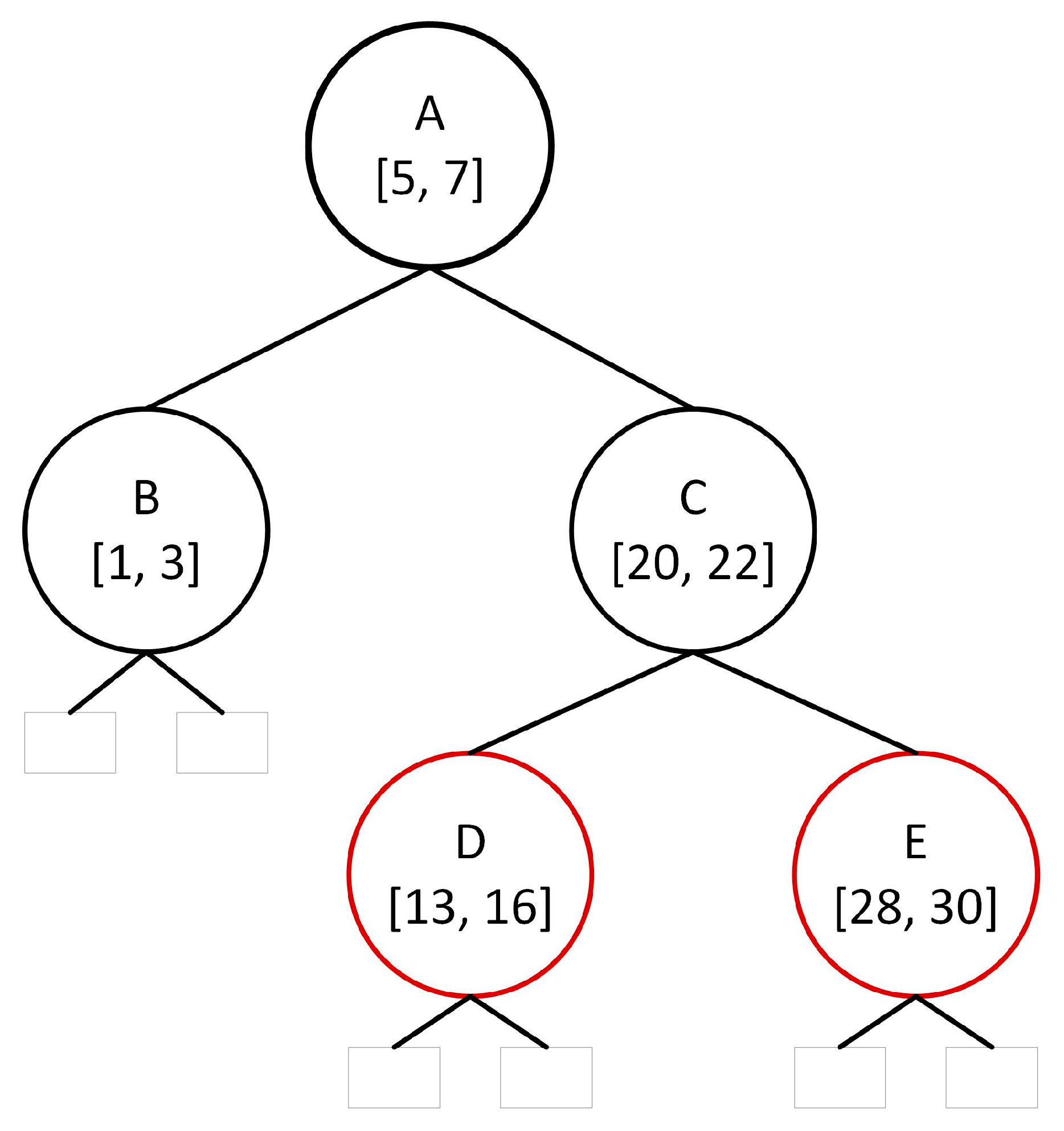
- Cormen, T.H.; Leiserson, C.E.; Rivest, R.L.; Stein, C. Red-Black Trees. In Introduction to Algorithms, 3rd ed.; The MIT Press: Cambridge, MA, USA, 2009; pp. 308–323. [Google Scholar]


| Symbol | Definition |
|---|---|
| Time is discretized every | |
| Fastest possible negative deceleration rate of all UAVs | |
| Fastest possible positive acceleration rate of all UAVs | |
| Minimum allowed distance between two UAVs | |
| Absolute value of | |
| Speed of | |
| Acceleration/deceleration rate of from to | |
| Distance travels from | |
| . | |
| when both have stopped in the lane | |
| until it stops | |
| until it enters the intersection | |
| Constant acceleration/deceleration rate uses from until it reaches the exit of the queueing zone | |
| Time spends waiting at the entrance of the acceleration zone | |
| spends in the acceleration zone | |
| Deceleration rate uses from such that its speed at the entrance of the acceleration zone equal to zero | |
| when it reaches the entrance of the acceleration zone | |
| spends to accelerate from to in the acceleration zone | |
| travels while accelerating from to . | |
| spends to reach the exit of the acceleration zone while maintaining its speed after reaching |
| Intersection Parameters |
|---|
| m/s |
| m/s |
| = −3.5 m/s2 |
| = 4 m/s2 UAV diameter is randomly assigned between 1 to 4 m |
| 190 m |
| 52 m |
| 46 m |
| 5 lanes per way Lane width = 5 m Intersection layer height = 5 m Intersection size = 50 m × 50 m Cube size = 1 m |
| Scheduling Parameters |
|---|
| s s |
| GA’s population size per generation = 100 GA’s number of generations = 50 |
| GA’s mutation rate = 10% |
| Intersection Parameters |
|---|
| m/s |
| m/s |
| Lane width = 5 m 3 lanes per way |
| Intersection size = 30 m × 30 m |
| Intersection Parameters |
|---|
| = −3.5 m/s2 |
| = 4 m/s2 |
| 150 m |
| 33 m |
| 29 m |
| Cell size = 1 m s |
| s |
| GA population size per generation = 100 GA termination = 80 generations |
| GA mutation rate = 10% |
Publisher’s Note: MDPI stays neutral with regard to jurisdictional claims in published maps and institutional affiliations. |
© 2022 by the authors. Licensee MDPI, Basel, Switzerland. This article is an open access article distributed under the terms and conditions of the Creative Commons Attribution (CC BY) license (https://creativecommons.org/licenses/by/4.0/).
Share and Cite
Rubenecia, A.; Choi, M.; Choi, H.-H. Reservation-Based 3D Intersection Traffic Control System for Autonomous Unmanned Aerial Vehicles. Electronics 2022, 11, 309. https://doi.org/10.3390/electronics11030309
Rubenecia A, Choi M, Choi H-H. Reservation-Based 3D Intersection Traffic Control System for Autonomous Unmanned Aerial Vehicles. Electronics. 2022; 11(3):309. https://doi.org/10.3390/electronics11030309
Chicago/Turabian StyleRubenecia, Areeya, Myungwhan Choi, and Hyo-Hyun Choi. 2022. "Reservation-Based 3D Intersection Traffic Control System for Autonomous Unmanned Aerial Vehicles" Electronics 11, no. 3: 309. https://doi.org/10.3390/electronics11030309