
Polynomial Algorithm for Minimal (1,2)-Dominating Set in Networks


Department of Algorithms and Systems Modelling, Faculty of Electronics, Telecommunications and Informatics, Gdańsk University of Technology, Narutowicza 11/12, 80-233 Gdańsk, Poland
Electronics 2022, 11(3), 300; https://doi.org/10.3390/electronics11030300
Submission received: 30 December 2021
/
Revised: 13 January 2022
/
Accepted: 17 January 2022
/
Published: 19 January 2022
(This article belongs to the Special Issue 10th Anniversary of Electronics: Recent Advances in Computer Science & Engineering)
Abstract
:Dominating sets find application in a variety of networks. A subset of nodes D is a -dominating set in a graph if every node not in D is adjacent to a node in D and is also at most a distance of 2 to another node from D. In networks, -dominating sets have a higher fault tolerance and provide a higher reliability of services in case of failure. However, finding such the smallest set is NP-hard. In this paper, we propose a polynomial time algorithm finding a minimal -dominating set, Minimal_12_Set. We test the proposed algorithm in network models such as trees, geometric random graphs, random graphs and cubic graphs, and we show that the sets of nodes returned by the Minimal_12_Set are in general smaller than sets consisting of nodes chosen randomly.
1. Introduction
In networks, some resources (possibly limited in number) should be available immediately and directly. Thus, some nodes can function as special nodes, for example, servers, radio broadcasting stations, schools or hospitals in networks of streets, and towns or countries. Then these special nodes form a dominating set. Since we want to minimize the total costs of devices, facilities or buildings, we are interested in dominating sets of small cardinality. The domination number is the number of the smallest possible number of these special nodes.
However, some networks demand a higher reliability, so in the case of one server’s failure, a different one can take over necessary tasks. In this paper, we focus on a situation when a spare special node does not need to be a direct neighbour of an ordinary node—it might be at distance of 1 or 2. If a spare special node is at distance 2, then the communication might be performed at a lower speed or only the most demanding tasks may be assured by the spare server. An analogous situation takes place when the poor signal coverage (because of a failure) makes it impossible to make standard connections via a mobile phone network. However, in most situations we can call emergency numbers. During pandemics we want to be sure that in case of overcrowding of the nearest hospital, there is a spare one at most two distances further. Similar situation takes place when we want to manage the location of maternity wards. To fulfil these conditions, the special nodes need to form a -set, also known as a secondary dominating set. Of course, determining the smallest -set is most desirable.
The execution time of a polynomial–time algorithm can be bounded by from above by a polynomial on the size of the input. For this reason such algorithms have practical use in networks. The Information System on Graph Classes and their Inclusions [1] shows what we know about computational complexity of graph theory problems. It can be noted that for most types of dominating set problems determining the smallest set of the desired property is NP-hard in general graphs. This means that polynomial algorithms solving these problems are not known (for more information about NP-hard problems and polynomial algorithms see [2]). On the other hand, polynomial–time algorithms exist for specific graph classes. For example, finding the minimum domination number is polynomial in trees, block graphs, interval graphs, cographs and permutation graphs (sample algorithms with examples can be found in [3,4]).
For wider and more general graph classes approach on the other way can be made. Approximate polynomial algorithms are developed, however they do not ensure that the returned results are best possible, that is of smallest cardinality and dominating at the same time. Since -dominating sets have potential for many applications in real-life situations and up to now there is a little known about algorithms finding these sets, in our paper we propose a polynomial time algorithm that finds a minimal -dominating set in any graph. Such a set can be regarded as good heuristic of the minimum (the smallest) -dominating set (see Section 3.1 for more details on minimum and minimal sets and Section 4.2 for results for trees).
This paper is organized as follows. In Section 3, we present the formal definitions used in a model of a network and we state the difference between minimum and minimal sets. Next we present algorithms PowerOfNodes and Minimal_12_Set. In Section 4, we analyze the performance of the algorithms in geometric random graphs in which nodes are placed randomly on a unit square and two nodes are adjacent if and only if the distance between them in Euclidean space is at most given threshold. This is done to predict the results given by the algorithm in a real network situation. Moreover, we compare the results returned by the algorithm with exact values of -domination number in tree graphs. This helps us check how much the algorithm is better than simply choosing nodes randomly. At last, we investigate performance of the algorithm in random graphs and cubic graphs. In Section 6, we give conclusion of this paper and discuss future further works.
2. Related Works
A review of the literature shows that domination parameters can be used in many applications, ranging from diverse sensor networks [5] to vehicular ad hoc communications [6,7], DNA sequencing [8], safety and reliability in transportation [9], disaster rescue operations [10], and many others. In all these works graphs are used to model the network. In case of Wireless Sensor Networks, mainly dominating sets, connected dominating sets and weakly connected dominating sets are studied. The connected dominating set is a model of a virtual backbone, which helps achieve efficient broadcasting in these networks [11,12]. Connected domination has also applications to ad hoc networks and there are a few papers on this topic—see, for example [6,13].
Until now, there have not been many papers on domination. The concept of -dominating sets in graphs was introduced by Hedetniemi et al. [14] as secondary domination. They also generalized this notion to -domination, where k is a positive integer. In [15], the authors study -domination number in tournaments, and in [16] graphs with the -domination number close to their orders are characterized. An independent version of -domination in graphs is studied in [17]. In particular the authors investigate graphs which posses a -dominating set such that no two nodes of the set are adjacent.
The computational complexity of determining the smallest -dominating sets in graphs and a polynomial time algorithm finding the -domination number in trees are presented in [18]. In particular, the authors prove that determining the -dominating number is NP complete, even for split graphs and even for bipartite graphs and many other graph classes. In the same paper, the author prove that if a graph does not have nodes of degree one nor triangles (three nodes such that each two of them are adjacent), then the -domination number is equal to the domination number. The problem is that determining the domination number is also NP-hard. Furthermore, in the case of ad hoc networks, we may never be sure whether the network contains triangles of nodes of degree one without constant checking the structure of the network.
The main differences between this contribution and published works is that the published works do not consider approximate algorithms that find the -domination number for general graphs. Even though there are some algorithms for dominating sets and connected dominating sets (for example a self-stabilizing algorithm finding a minimal dominating set is presented in [19] and an exact algorithm for the domination number is given in [20], however it runs in exponential time) they can not be applied to -domination. By the definition, -domination number is never bigger than domination number. Similarly, if the connected domination number of a graph is equal to 1, then the -domination number is equal 2, however in all other cases the -domination number is not greater than the connected domination number. Moreover, the difference between these two dominating numbers may be big relative to the number of nodes (for a path on 100 nodes the difference between these two domination parameters is 64). Hence, we conclude that algorithms for connected dominating sets do not apply here.
Since determining the exact value of -domination number is known to be NP-hard for chordal bipartite graphs, -free graphs, maximum degree 4 graphs, partial grid graphs and planar graphs (see [18]), in this paper we propose an algorithm that finds a minimal -dominating set in an arbitrary graph in a polynomial time. By analyzing neighbourhoods of nodes, our algorithm aims to construct a minimal -dominating sets of cardinalities close to the -domination number.
3. Materials and Methods
In this section, we explain all necessary definitions and also indicate the difference between the minimum and minimal -dominating sets. Next, we present the two main algorithms of this work.
3.1. Model of Network
In a formal way, let an undirected graph be a model of a network. Namely, let V be the set of nodes and E the set of two element subsets of V, called links. If is a link, then we will write for short. If , then is the set of all neighbours of v and is the set of nodes in G at distance exactly 2 from v, that is . The number of elements in is called the degree of v.
A set is a dominating set in of graph if every node not in D is adjacent to a node in D. A set is a -dominating set in G if every node not in D is adjacent to a node in D and is also at distance at most 2 to another node from D. Hence each -dominating set is also a dominating set, but not vice versa. The -domination number, denoted by , is the cardinality of a smallest -dominating set of G.
We say that a node v is -dominated by a subset if v is adjacent to a node belonging to D and there is another node in D at distance at most 2 from v.
A -dominating set is a minimal -dominating set of a graph G if no proper subset of D is a -dominating set of a G. The following example clarifies the difference between minimum and minimal -dominating sets.
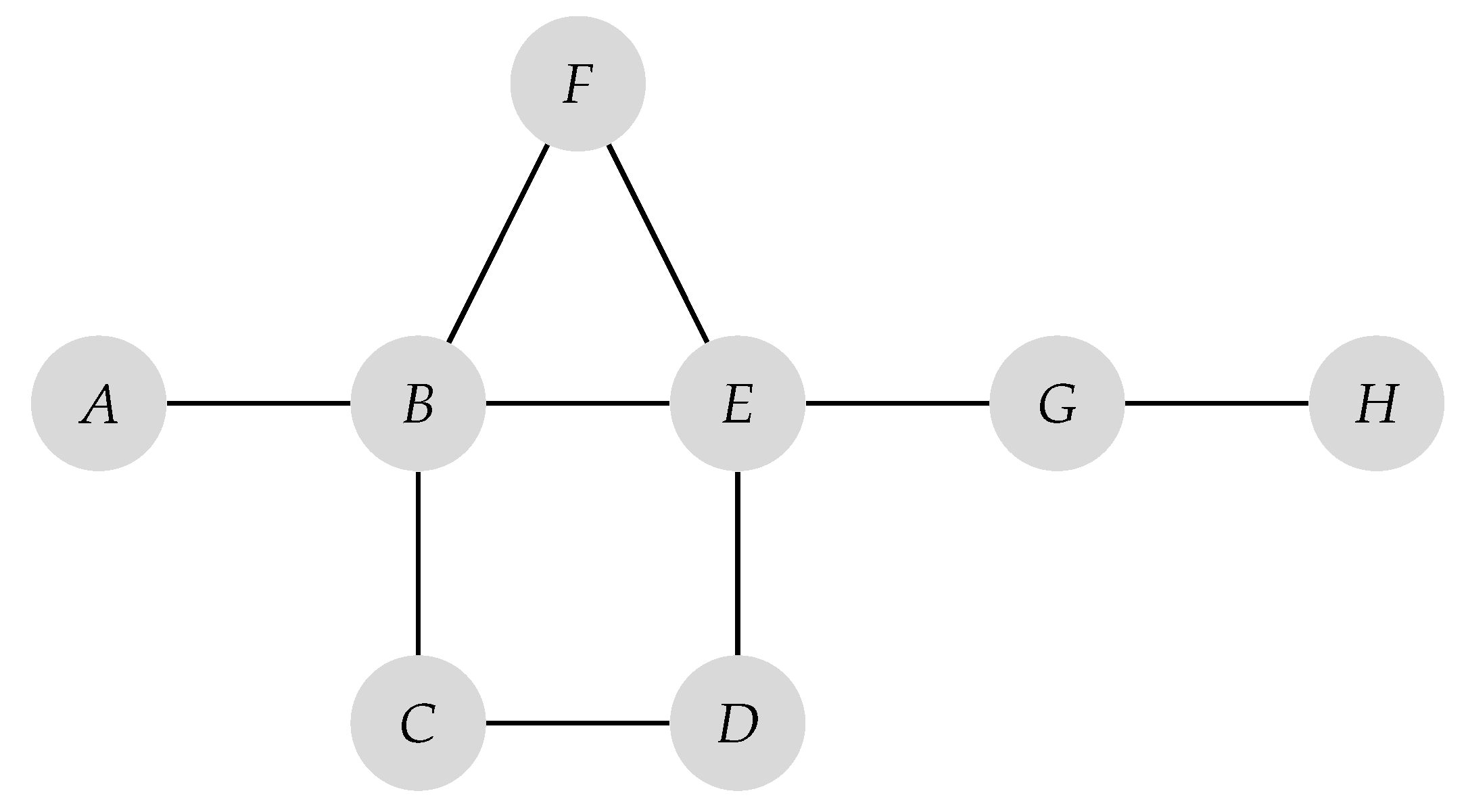
For example, in Figure 1 the sets and are examples of minimal -dominating sets, but only the sets with three nodes are minimum -dominating sets. The set is not a -dominating set, as although H has a neighbour in this set (namely G), no other node of the set is at distance at most 2 from H. On the other hand, a set is a -dominating set, but not minimal, because its proper subset, is also a -dominating set.
In some cases, in graph G the difference between the -domination number and a cardinality of a minimal -dominating set can be large in relation to the number of nodes of G. For example, let us consider a star with t nodes of degree 1. Then , while the set of all nodes of degree 1 form the biggest minimal -dominating set. The algorithm presented in this paper tries to avoid constructing such a biggest minimal -dominating sets. In particular, for stars it always returns a solution with two nodes, which is the best in terms of the number of nodes.
3.2. Algorithm PowerOfNodes
The algorithm presented here finds a minimal -dominating set D in G. In the beginning, D is an empty set. In each main step of the algorithm, a new node is added to D until each node in has a neighbour in D as well as is at distance at most 2 to another node in D.
Each node has three local variables: , and . These variables show the state of each node and its neighbours.
- If a node v is chosen to be in D, then is equal to 1. Otherwise, .
- If , then .If and if additionally
- For each node x of is , then .
- There is exactly one node x in such that and for each node x of is , then .
- There is at least one node x in , such that and for each node x of is , then .
- v is -dominated by nodes in D, then .
- This parameter shows the gain of adding v to D and its value depends on two algorithm parameters: and . If v is already chosen to the -dominating set, then . Otherwise, , where
- if v is not -dominated and otherwise .
- is the number of nodes in that do not have a neighbour in D.
- is the number of nodes in that have exactly one neighbour in D but are not -dominated by D or do not have any neighbours belonging to D within distance 2.
By assigning different values to parameters we can obtain different -dominating set D.
To introduce an algorithm for finding a minimal -dominating set in arbitrary graphs, we first introduce a function PowerOfNodes which has four parameters: a graph G, a node and two positive numbers: . The function determines the powers of u, each neighbour of u and each node at distance 2 from u.
Algorithm PowerOfNodes Analysis
Let v be a node in . The Algorithm 1 first checks (if...else lines 3 and 14–15) whether v is in D (then the power of v is always 0) or not. If not and if v is not -dominated, then v gets power at least 1 (lines 5–6). This assures a proper work of the Algorithm 1 in case when, for example, v is not connected to any other node.
| Algorithm 1:PowerOfNodes |
 |
For each node not in D belonging to with code 0 or 10, we add to (lines 7–9). Similarly, for each node not in D belonging to with code smaller than 11, we add to (lines 10–12). Hence, a node gains a higher power if it has more non -dominated nodes in its neighbourhoods. By assigning different values to , we may obtain different results.
Since there might be some links among nodes in , the algorithm not only updates the power of v, but also nodes in . For this reason the complexity of this algorithm is , where is the maximum degree of a node in a graph.
3.3. Algorithm Minimal_12_Set
The second algorithm, namely Minimal_12_Set uses the PowerOfNodes algorithm and finds a minimal -dominating set.
Algorithm Minimal_12_Set Analysis
In the beginning, Algorithm 2 assigns initial values to nodes: and are assigned 0, while of a node v is a positive number and is equal to (lines 2–5). In each step of the main loop of the Minimal_12_Set (while...do lines 6–20), a node with the maximum value of is chosen and added to the minimal -dominating set (lines 7–11). This node changes its value of from 0 to 1 (line 12). Then, necessary local variables of nodes are updated, first (lines 14–19), then (line 20). Checking whether (line 11) prevents the addition of a redundant node to the minimal -dominating set. At the end of the performance of the Algorithm 2 (line 21), nodes with equal to 1 form a minimal -dominating set.
Note that in the case of assigning the powers of nodes at distance at most 4 might change. Our algorithm updates only powers of nodes at distance at most 2 from x (see the Minimal_12_Set algorithm). This accelerates the performance of the algorithm. However lines 7–11 make sure that the set of nodes with is always minimal in sense of -domination.
| Algorithm 2:Minimal_12_Set |
 |
The main loop of the Algorithm 2 (while...do lines 6–20) performs at most times, because each time it adds one node to the -dominating set and nodes in the -dominating set have . Moreover, it takes at most operations to choose a node with the highest power and at most operations to update the power of a node and nodes at distance 1 or 2 from it. Therefore, the time complexity for Algorithm 2 is , so it is polynomial.
3.4. Example
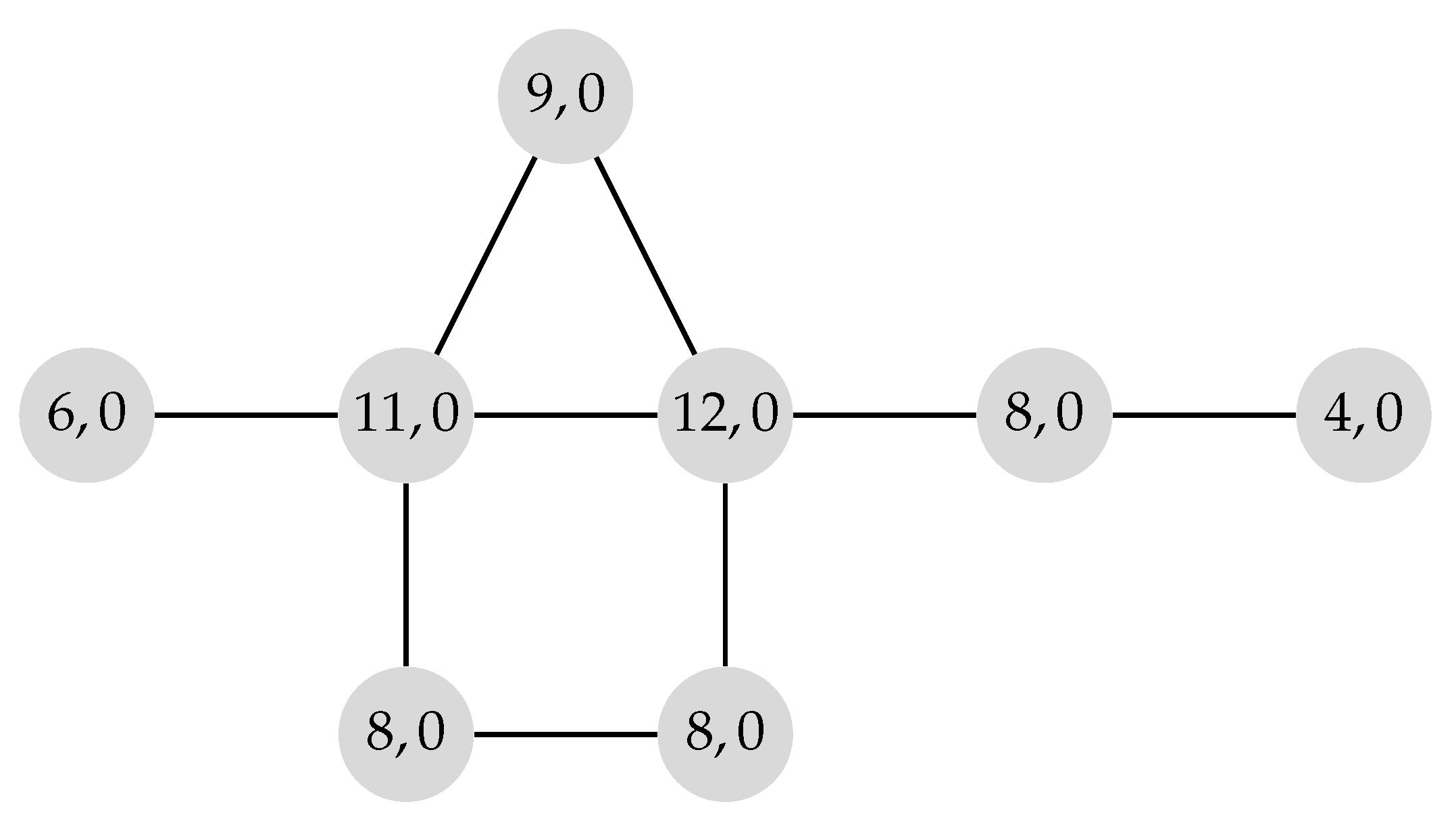
We illustrate the performing of the Minimal_12_Set for and . Let G be a graph as in Figure 2. The first number inside a node is its power, while the second–code. The numbers in Figure 2 show their values after performing the first five lines of the Algorithm 2.
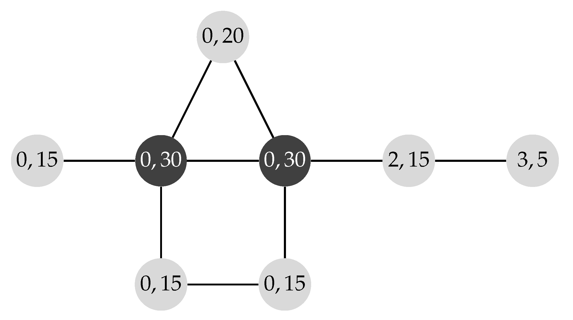
The graph in Figure 3 illustrates the state of the graph after performing the main while...do loop (lines 6–20) once. The dark node has and the light have .
The state of the graph after performing the main loop twice is presented in Figure 4. Note that since the node of degree 1 and is at distance more than 2 from the node lastly added to the -dominating set, its power is not updated.
The graph G after the last, third performance of the main loop is shown in Figure 5. The power of each node is 0. Since , in this example the Minimal_12_Set algorithm finds a minimal -dominating set with the minimum possible cardinality.
4. Results
The Minimal_12_Set algorithm and PowerOfNodes function were implemented and tested using the igraph library in R. First, we used random geometric graphs as models of a network. A geometric random graph is the model of a spatial network, namely an undirected graph, constructed by placing randomly a given number of nodes in a unit square and connecting two nodes by a link if and only if their distance is in a given range, see [21,22]. In our tests, we generated random geometric graphs of order from 55 to 190 nodes and the radius within which the nodes are connected by a link between 0.08 and 0.4. We used three sets of parameters:
- denoted 2 1,
- denoted 1 1,
- denoted 1 2.
For each graph we compared the results obtained by Minimal_12_Set with an algorithm that builds a minimal -dominating set by choosing a permitted node randomly. (We permit a node to be added to a minimal -dominating set if adding this node decreases the number of nodes which are not partially or fully -dominated). We call this algorithm a random algorithm and denote it on presented diagrams by rand. Its time complexity is .
Next, since there is an optimal algorithm finding the -domination number in trees [18], we checked the performance of the algorithm for this class of graphs and we compared the results with an optimal solution as well as with the results returned by the random algorithm. Since adding a new link to a graph does not increase its -domination number, the -domination number of a spanning tree of a connected graph G is an upper bound for the -domination number of G. At last we shortly study the performance of our algorithm in random graphs and cubic graphs.
The statistics are done in Python using the pandas [23] library and the visualization with the seaborn [24] library.
4.1. Geometric Random Graphs
As it is shown in Figure 6, the Minimal_12_Set algorithm gave much better results than the random algorithm in the case of geometric random graphs. Not surprisingly, the difference between the results of the algorithms was greater for graphs with more nodes.
In most cases of our tests, the algorithm with parameters 2 1 gave the best results on average, however the differences between versions 2 1, 1 1 and 1 2 were not significant.
4.2. Trees
The Minimal_12_Set algorithm analyzes local neighbourhoods of each node. For this reason, for example in stars it always finds a minimal -dominating set with the smallest possible cardinality, namely a minimum -dominating set. However, this may not be true for trees in general.
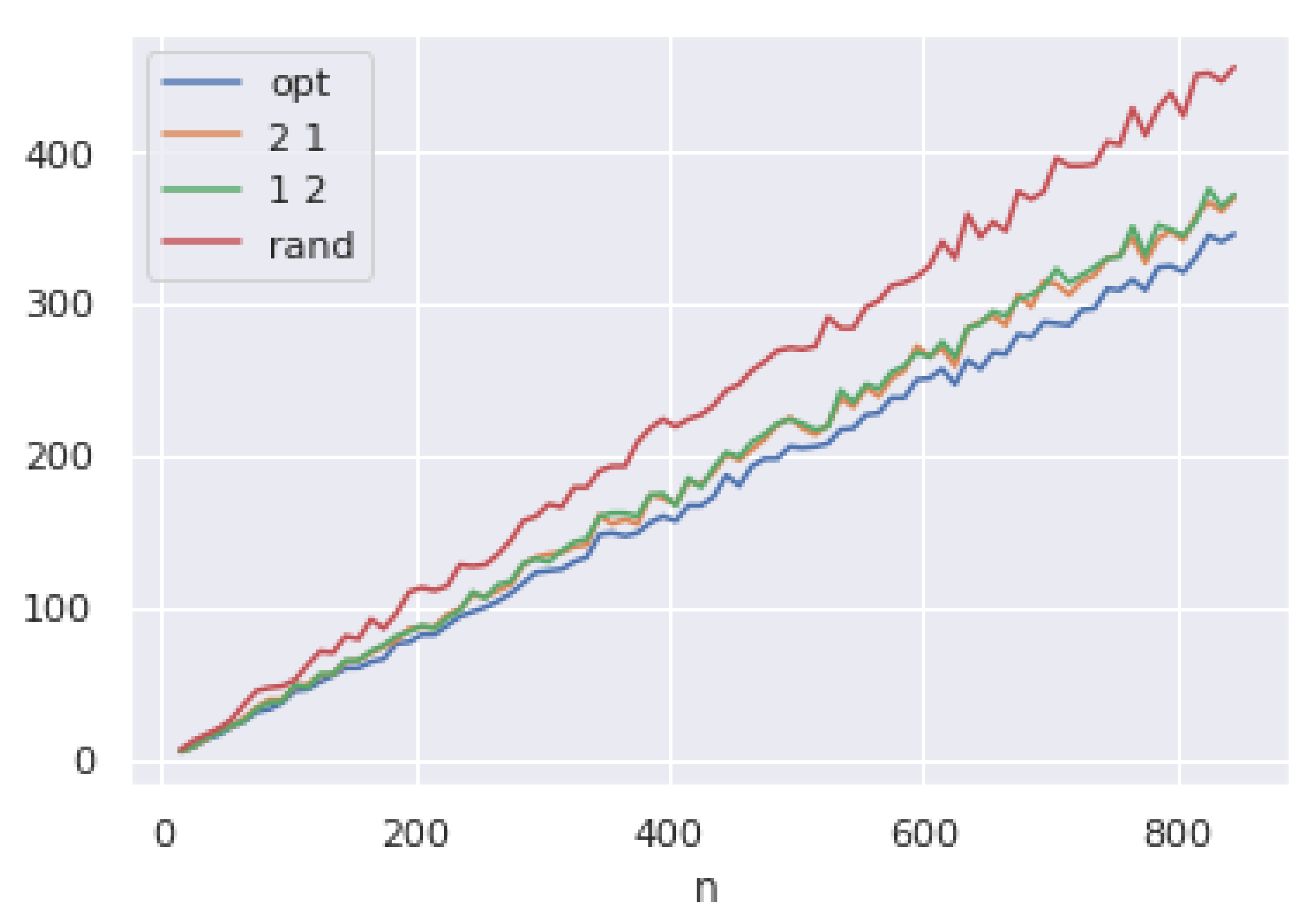
We tested the algorithms on random trees of order from 15 to 845 nodes. The results given by the Minimal_12_Set algorithm and the random algorithm were compared to the optimal algorithm that finds the -domination number in trees (for details of the optimal algorithm see [18]). The cardinalities of the minimal -dominating sets together with the optimal solutions are given in Figure 7.
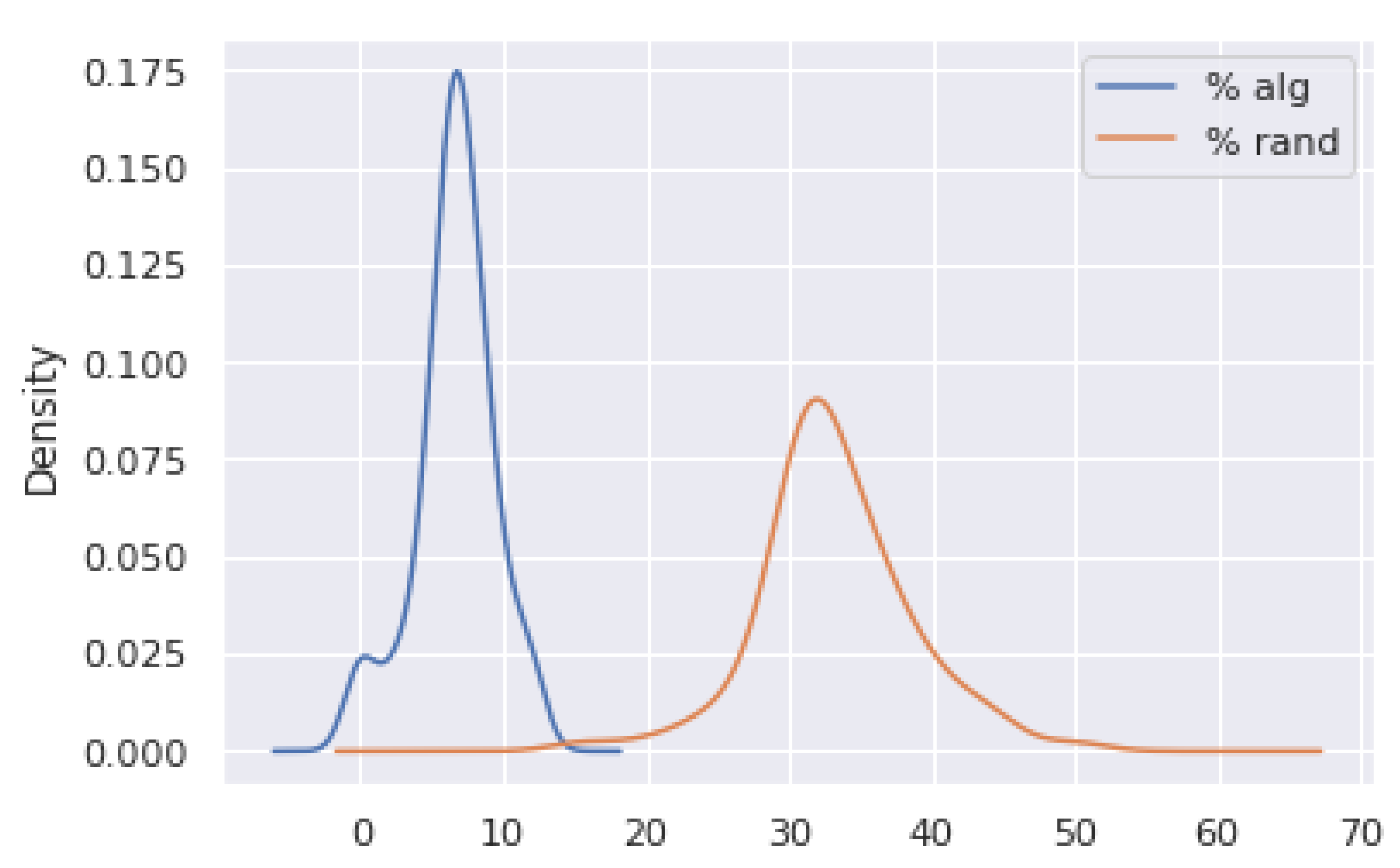
It can be seen that the differences between the values returned by the Minimal_12_Set algorithm and the exact algorithm were much smaller than for the case of random algorithm. To investigate this difference more deeply, we counted the percent error. Namely, Figure 8 shows the percent error of the minimum value returned by algorithms 2 1 and 1 2 in relation to the optimal solution (denoted % alg), as well as the percent error of the random algorithm (denoted % rand). We noted that the Minimal_12_Set algorithm gives much better results than the random one.
The statistics presented in Table 1 show that the percent error of 2 1 and 1 2 is relatively small, because it lies between and with a mean value of , while the percent error of the random algorithm is between and with a mean value of .
4.3. Random Graphs and Regular Graphs
We have tested the algorithm for random graphs generated according to the Erdos–Renyi model for n varying from 30 to 250 and the probability for constructing a link . The results can be seen in Figure 9.
The statistics show that the random algorithm returned values on average worse than the Minimal_12_Set algorithm. Moreover, the results given by the random algorithm were more diverse. In some cases the results were just worse than the Minimal_12_Set algorithm, while in some cases were as high as worse.
Since the Minimal_12_Set algorithm prefers the nodes with the highest degree, we tested the Minimal_12_Set algorithm and random algorithm on random cubic graphs, that is graphs in which each node is of degree 3. We supposed that these graphs should eliminate the advantage of adding nodes with high degrees to the minimal -dominating set. Since the degree of each node is only 3, adding a node to a minimal -dominating set changes the power of at most 10 nodes. We tested the algorithms for cubic graphs of order from 30 to 500 nodes. Furthermore, in this situation the Minimal_12_Set algorithm gave better results than the random one. The random algorithm gave worse results by on average, varying from to .
5. Discussion
In this paper, we proposed two algorithms: PowerOfNodes and Minimal_12_Set. The second algorithm uses the first one and finds, in a polynomial time, a minimal -dominating set of any graph. The conducted tests in trees show that the results returned by the Minimal_12_Set are not far from the optimal solution and are much better than a simple random algorithm. Since a tree is a subgraph of any graph, this allows us to assume that similar good results should be true in general graphs. The tests performed for geometric random graphs, random graphs and cubic graphs seem to confirm our suppositions. Even though the nodes in cubic graphs have the same degree, the new algorithm still returned better results than the random one.
For these reasons, our algorithm may be used in high reliability networks in which we must guarantee that each node has an instant access to a spare server at least at distance 2 from it. Since each node has a spare dominating node in -dominating set, these networks are more fault tolerant. Additionally, if the model of a network is vast, there is a possibility of dividing it into unit squares and applying the algorithm in each square independently.
6. Conclusions and Future Work
In future, it might be interesting to investigate the potential of using the Minimal_12_Set algorithm in ad hoc networks in which nodes are changing their positions. Furthermore, it is worth checking whether updating the powers of all nodes at distance at most 4 from the node newly added to the minimal -dominating set will give much better results than updating the powers of nodes at distance at most 2. Of course, the computational time complexity of the new version of the algorithm will be greater, so the question is if such greater time complexity is of practical importance.
Another interesting open problem is to investigate possible generalization of the presented algorithms to -domination. In this paper, we are studying the case for , however other values of k seems to be worth studying. The possible extension of the algorithm for the neural networks and neuromorphic computing is left for further investigations in future.
Funding
This work was supported by the Ministry Subsidy for Research for Gdańsk University of Technology.
Data Availability Statement
Datasets analyzed or generated during the study. https://github.com/JoannaRaczek/Polynomial-Algorithm-for-Minimal-1-2-Dominating-Set, accessed on 18 December 2021.
Conflicts of Interest
The authors declare no conflict of interest.
References
- Information System on Graph Classes and Their Inclusions (ISGCI). Available online: https://www.graphclasses.org (accessed on 18 December 2021).
- Garey, M.R.; Johnson, D.S. Computers and Intractability: A Guide to the Theory of NP-Completeness; Freeman: San Francisco, CA, USA, 1979. [Google Scholar]
- Haynes, T.W.; Hedetniemi, S.T.; Slater, P. Fundamentals of Domination in Graphs, 1st ed.; CRC Press: Boca Raton, FL, USA, 1998. [Google Scholar] [CrossRef]
- Haynes, T.W.; Hedetniemi, S.T.; Slater, P.J. Domination in Graphs Advanced Topics, 1st ed.; Routledge: London, UK, 1998. [Google Scholar] [CrossRef]
- Karbasi, A.H.; Atani, R.E. Application of Dominating Sets in Wireless Sensor Networks. Int. J. Secur. Its Appl. 2013, 7, 185–202. [Google Scholar]
- Dubois, S.; Kaaouachi, M.H.; Petit, F. Enabling Minimal Dominating Set in Highly Dynamic Distributed Systems. In Stabilization, Safety, and Security of Distributed Systems; Pelc, A., Schwarzmann, A., Eds.; SSS 2015, Lecture Notes in Computer Science; Springer: Cham, Switzerland, 2015; Volume 9212. [Google Scholar] [CrossRef] [Green Version]
- Yu, J.; Wang, N.; Wang, G.; Yu, D. Connected dominating sets in wireless ad hoc and sensor networks—A comprehensive survey. Comput. Commun. 2013, 36, 121–134. [Google Scholar] [CrossRef]
- Yamuna, M.; Karthika, K. Medicine names as a DNA sequence using graph domination. Pharm. Lett. 2014, 6, 175–183. [Google Scholar]
- Guze, S. An application of the selected graph theory domination concepts to transportation networks modelling. Sci. J. Marit. Univ. Szczec. 2017, 52, 97–102. [Google Scholar]
- Ramalakshmi, R.; Radhakrishnan, S. Weighted dominating set based routing for ad hoc communications in emergency and rescue scenarios. Wirel. Netw. 2015, 21, 499–512. [Google Scholar] [CrossRef]
- Hedar, A.-R.; Abdulaziz, S.N.; Mabrouk, E.; El-Sayed, G.A. Wireless Sensor Networks Fault-Tolerance Based on Graph Domination with Parallel Scatter Search. Sensors 2020, 20, 3509. [Google Scholar] [CrossRef] [PubMed]
- Hedar, A.-R.; El-Sayed, G.A. Parallel genetic algorithm with elite and diverse cores for solving the minimum connected dominating set problem in wireless networks topology control. In Proceedings of the 2nd International Conference on Future Networks and Distributed Systems (ICFNDS ’18), New York, NY, USA, 26–27 June 2018; Association for Computing Machinery: New York, NY, USA, 2018; pp. 1–9. [Google Scholar] [CrossRef]
- Dai, F.; Wu, J. An extended localized algorithm for connected dominating set formation in ad hoc wireless networks. IEEE Trans. Parallel Distrib. Syst. 2004, 15, 908–920. [Google Scholar] [CrossRef]
- Hedetniemi, S.M.; Hedetniemi, S.T.; Kinsley, J.; Rall, D.F. Secondary Domination in Graphs. AKCE J. Graphs Combin. 2008, 5, 103–115. [Google Scholar]
- Factor, K.A.S.; Langley, L.J. An introduction to (1,2)-domination graphs. Congr. Numer. 2009, 199, 33–38. [Google Scholar]
- Kayathri, K.; Vallirani, S. (1,2)-Domination in Graphs. In Theoretical Computer Science and Discrete Mathematics; Arumugam, S., Bagga, J., Beineke, L., Panda, B., Eds.; ICTCSDM 2016, Lecture Notes in Computer Science; Springer: Cham, Switzerland, 2017; Volume 10398. [Google Scholar] [CrossRef]
- Michalski, A.; Włoch, I. On the existence and the number of independent (1,2)-dominating sets in the G-join of graphs. Appl. Math. Comput. 2020, 377, 125155. [Google Scholar] [CrossRef]
- Raczek, J. Complexity Issues on Secondary Domination Number. Nord. J. Comput. 1994, 1, 157–171. [Google Scholar]
- Kakugawa, H.; Masuzawa, T. A self-stabilizing minimal dominating set algorithm with safe convergence. In Proceedings of the 20th IEEE International Parallel and Distributed Processing Symposium, Rhodes, Greece, 25–29 April 2006; p. 8. [Google Scholar] [CrossRef]
- van Rooij, J.M.M.; Bodlaender, H.L. Exact algorithms for dominating set. Discr. Appl. Math. 2011, 159, 2147–2164. [Google Scholar] [CrossRef] [Green Version]
- Penrose, M. Random Geometric Graphs; Oxford Univ. Press: Oxford, UK, 2003. [Google Scholar] [CrossRef]
- Bringmann, K.; Friedrich, T. Exact and Efficient Generation of Geometric Random Variates and Random Graphs. In Automata, Languages, and Programming; Fomin, F.V., Freivalds, R., Kwiatkowska, M., Peleg, D., Eds.; ICALP 2013, Lecture Notes in Computer Science; Springer: Berlin/Heidelberg, Germany, 2013; Volume 7965. [Google Scholar] [CrossRef] [Green Version]
- Pandas. Available online: https://pandas.pydata.org/ (accessed on 2 October 2021).
- Seaborn: Statistical Data Visualization. Available online: https://seaborn.pydata.org/ (accessed on 2 October 2021).
Figure 1.
Example of a graph.

Figure 2.
Graph G at line 5 of the Algorithm 2.

Figure 3.
Graph G after performing the main loop of the Algorithm 2 once.

Figure 4.
Graph G after performing the main loop of the Algorithm 2 twice.

Figure 5.
Graph G after performing the main loop of the Algorithm 2 third (and last) time.

Figure 6.
Average number of nodes in a minimal -dominating set.

Figure 7.
Returned values of carnality of minimal -dominating sets for random trees.

Figure 8.
Percent error.

Figure 9.
The cardinality of -dominating sets returned by the Minimal_12_Set and random algorithms in random graphs.
Figure 9.
The cardinality of -dominating sets returned by the Minimal_12_Set and random algorithms in random graphs.


Table 1.
Basic statistics for percent error.
| % Alg | % Rand | |
|---|---|---|
| mean | 6.636940 | 33.234861 |
| std | 2.700715 | 5.330012 |
| min | 0.000000 | 15.555556 |
| 25% | 5.559414 | 30.740952 |
| 50% | 6.698718 | 32.365320 |
| 75% | 8.016610 | 35.875975 |
| max | 12.121212 | 50.000000 |
Publisher’s Note: MDPI stays neutral with regard to jurisdictional claims in published maps and institutional affiliations. |
© 2022 by the author. Licensee MDPI, Basel, Switzerland. This article is an open access article distributed under the terms and conditions of the Creative Commons Attribution (CC BY) license (https://creativecommons.org/licenses/by/4.0/).
Share and Cite
MDPI and ACS Style
Raczek, J. Polynomial Algorithm for Minimal (1,2)-Dominating Set in Networks. Electronics 2022, 11, 300. https://doi.org/10.3390/electronics11030300
AMA Style
Raczek J. Polynomial Algorithm for Minimal (1,2)-Dominating Set in Networks. Electronics. 2022; 11(3):300. https://doi.org/10.3390/electronics11030300
Chicago/Turabian StyleRaczek, Joanna. 2022. "Polynomial Algorithm for Minimal (1,2)-Dominating Set in Networks" Electronics 11, no. 3: 300. https://doi.org/10.3390/electronics11030300
Note that from the first issue of 2016, this journal uses article numbers instead of page numbers. See further details here.