A DEXiRE for Extracting Propositional Rules from Neural Networks via Binarization

Abstract

Background: Despite the advancement in eXplainable Artificial Intelligence, the explanations provided by model-agnostic predictors still call for improvements (i.e., lack of accurate descriptions of predictors’ behaviors). Contribution: We present a tool for Deep Explanations and Rule Extraction (DEXiRE) to approximate rules for Deep Learning models with any number of hidden layers. Methodology: DEXiRE proposes the binarization of neural networks to induce Boolean functions in the hidden layers, generating as many intermediate rule sets. A rule set is inducted between the first hidden layer and the input layer. Finally, the complete rule set is obtained using inverse substitution on intermediate rule sets and first-layer rules. Statistical tests and satisfiability algorithms reduce the final rule set’s size and complexity (filtering redundant, inconsistent, and non-frequent rules). DEXiRE has been tested in binary and multiclass classifications with six datasets having different structures and models. Results: The performance is consistent (in terms of accuracy, fidelity, and rule length) with respect to the state-of-the-art rule extractors (i.e., ECLAIRE). Moreover, compared with ECLAIRE, DEXiRE has generated shorter rules (i.e., up to $74\%$ fewer terms) and has shortened the execution time (improving up to $197\%$ in the best-case scenario). Conclusions: DEXiRE can be applied for binary and multiclass classification of deep learning predictors with any number of hidden layers. Moreover, DEXiRE can identify the activation pattern per class and use it to reduce the search space for rule extractors (pruning irrelevant/redundant neurons)—shorter rules and execution times with respect to ECLAIRE.

1. Introduction

Deep learning (DL) comprises a set of machine learning (ML) methods based on artificial neural networks (ANN) that can learn complex representations directly from input data through representation learning [1,2]. DL techniques are employed in complex tasks where manual feature engineering can be time-consuming or impossible to design. Moreover, DL architectures can be generalizable, and pre-trained DL models can be used across domains. For example, DL predictors have been adopted in numerous applications, including image processing [3], recommender systems [4], cyber-security [5], natural language processing [6], and in multiple decision support systems (DSS) [7]. DSS can strongly influence and persuade individuals and organizations. This raises ethical concerns about trust, privacy, and accuracy [8], as well as legal questions about liability, transparency, and risk exposition [9]. Therefore, DSS’s inner workings of the principles/mechanisms and outcomes must be intelligible to accept the DSS conclusions.

Interpreting and explaining DL predictors (both from human [10] and virtual agents [11,12] perspectives) have been, to date, widely investigated in the discipline named eXplainable Artificial Intelligence (XAI) [13]. XAI methods can be categorized into intrinsically interpretable (interpretable by design—i.e., decision trees [14], linear regression [15], and rule sets [15,16]), and post-hoc explainable (predictors trained on inputs–outputs—i.e., LIME [17], SHAPLEY [18], ECLAIRE [19], and CIU [20]).

Despite the significant advances in XAI, the quality of the explanations still calls for improvements. For example, on the one hand, model-agnostic approaches do not provide highly accurate descriptions of the predictor’s internal behavior. Instead, they focus solely on surrogate models (intrinsically interpretable models that mimic the original models) and ignore the internal structure of the actual model. On the other hand, model-specific approaches are restricted to a few DL architectures, limiting their scope of explanation. DL predictors are connectionist models that store their knowledge through a distributed structure represented by weighted connections between neurons and non-linear activation functions. Decompositional rule-extraction methods are suitable for extracting knowledge stored in the DL predictors. However, their scope is limited to specific architectures, usually one-hidden layer neural networks, and it is computationally expensive (requiring several phases of pruning and training).

This paper presents a tool for Deep Explanations and Rule Extraction (DEXiRE). Such a tool approximates rules for DL models with any number of hidden layers. The proposed approach employs binary neural networks to induce Boolean functions in the hidden layers, generating intermediate rule sets for every hidden layer. In turn, a rule set is inducted between the first hidden layer and the input layer. Finally, the complete rule set is obtained using inverse substitution on intermediate rule sets and first-layer rules. To reduce the size and complexity of the final rule set, the algorithm uses statistical tests and satisfiability algorithms to filter redundant, inconsistent, and non-frequent rules.

The rest of the paper is organized as follows:

Section 2 presents the state of the art on DL, XAI, and rule extraction from ANNs. Section 3 describes the methodology. Section 4 presents the experimental setup and the tests’ execution. Section 5 presents the experimental results. Section 6 discusses and evaluates the results and what we can learn from them. Finally, Section 7 concludes the paper.

2. State of the Art

The XAI contributions can be classified into two main branches: Explainable-by-design and Post-hoc Explanations [21,22].

As shown in Figure 1, on the one hand, decision trees, linear models, and rule-based approaches are considered explainable-by-design, meaning that the output is derived from the set of rules or thresholds within them. On the other hand, deep learning models, such as ANN, belong to post-hoc explanations, meaning that the output requires a third-party approach to be explained. Post-hoc explanations can be divided into local explanations (e.g., features importance) and global explanations (e.g., rule extraction). The concept of global or local explanations refers to interpreting a model from a different perspective. Global explanations focus on the model’s perspective, while local explanations focus on a particular data point or observation [21].

This paper focuses on rule-extraction approaches, which elicit the hidden knowledge embedded in DL predictors and help explain the ANN outcomes. Extracted rules can be used for hazard mitigation, traceability, system stability and fault tolerance, operational verification and validation, and more [23,24]. Andrews et al. [25] propose a multidimensional taxonomy for several rule-extraction methods, from shallow ANN architectures. They use the (i) decompositional approach: rule-extraction algorithms that work on the neuron level; (ii) pedagogical approach: rule-extraction algorithm regards the neural network as a black box; and (iii) eclectic approach: the combination of both decompositional and pedagogical approaches.

Decompositional algorithms work on the neuron level by extracting rules from neurons and inputting them into the whole network. In decompositional algorithms, every neuron and connection is transformed into a set of rules. A pioneer of decompositional algorithms is Fu [26,27], which proposed the KT algorithm and outlined the general algorithm by setting a threshold for each neuron. Fu resolved the problem by mapping the output result from each neuron (in hidden or output layers) into a Boolean function according to a given threshold. Towell and Shavlik [28] expanded the subset of Fu’s algorithm, which can extract M-of-N rules from MLP models. However, a significant complexity of computing time was added for finding all potential sets of links per neuron unit. The authors in [29] extracted rules from a neural network with one single hidden layer and one linear output unit for regression problems. The activation function in the hidden layer is approximately by piece-wise linear functions. To reduce the complexity, the network is pruned before rule extraction. Despite this limitation, the inherent simplicity of decompositional algorithms makes them extremely useful for explaining the mechanics of rule extraction and for providing interpretability of ANN models at the level of individual hidden and output units.

Pedagogical rule-extraction algorithms consider ANN as a black box, extracting based on the ANN’s inputs and outputs [30]—neurons and their connections are not subjected to analysis. The rules extracted using Pedagogical algorithms are directly extracted from the ANN’s output, which changes as the ANN’s input changes. Therefore, contrary to decompositional algorithms, the extracted rules are still intelligible if the ANN’s internal structure is complex. Thrun in [31] extracted symbolic knowledge rules from ANN based on Validity Interval Analysis by propagating the activations through the network. This technique simulates the ANN train coupling the system’s input and output patterns. HYPINV algorithm extracts rules from trained neural networks used in classification problems regardless of the structure of the network [32]. Model-agnostic methods, such as HYPINV, explain the predictions of arbitrary machine learning models independently of the implementation. They provide a way to explain predictors by considering models as black boxes. HYPINV approximates the network decision boundary by finding hyperplanes tangent to the decision hypersurface. Then the network decision boundary is represented in rules. Sethi et al. [30] proposed a pedagogical algorithm named KDRuleEx for rule extracting in the form of IF-THEN. The method can deal with discrete and continuous features and handles non-binary input. The authors in [33] compared rule sets extracted from ensembles of interpretable neural networks DIMLP, and their conclusion is that rule sets extracted from neural networks have greater accuracy than those extracted from decision tree ensembles but at a higher computational cost. The authors in [19] presented a new method to extract rules from Deep neural networks with any number of hidden layers. This efficient algorithm induces intermediate rule sets between the hidden layer and the predicted labels and with a process call-wise substitution to produce the final rule set.

Eclectic approach combines both the Decompositional and Pedagogical approaches. Most recent contributions in XAI are based on Eclectic approaches, such as Ebecken [34], which present the RX algorithm to extract rules from trained MLP in classification problems. RX (i) applies a clustering genetic algorithm to find clusters of hidden unit activation values, and (ii) generates classification rules describing these clusters w.r.t. the input. Local Interpretable Model-agnostic Explanations (LIME) [35] is a technique that explains how the input characteristics of an ML model affect its predictions. For instance, for image classification tasks, LIME seeks to find the region of an image (set of super-pixels) having the strongest association with a prediction label. LIME creates explanations by generating a new dataset of random disturbances (with their respective predictions) around the explained instance. Then it fits a weighted local surrogate model. This local model is usually simpler with inherent interpretability, such as a linear regression model. The first theoretical analysis of LIME was published in [36], confirming the crucial role of LIME, but also demonstrating its limitation (i.e., poor choice of parameters causes LIME to miss essential features).

In [37], authors concluded that pruning algorithms based on Mutual Information and Significance could be more efficient than the methods based on sensitivity and magnitude, as they consider the mutual dependency between the inputs of the network and outputs of the hidden neurons. This is a comparative study of pruning algorithms that compares six different algorithms of large variability with details explanations and uses only one three-class problem application (out of four) since it is the Iris dataset (popular and generally used in creating/testing algorithms) that might suggest that the results should be looked at critically.

Local Interpretable Visual Explanations (LIVE) [38] uses a surrogate model to predict the black box model’s local properties, generating the representative model’s coefficients. LIVE differs from LIME regarding local discoverability and how it handles interpretable inputs. LIVE does not create an interpretable input space by transforming input features but instead uses the original feature space. Since the shuffled data points correspond very closely to the original points, the similarity between them is measured using the identity kernel, while the original features are used as an interpretable input.

SHapley Additive exPlanations (SHAP) [39] is a game theory-inspired method that tries to improve interpretability by calculating the importance of each feature in individual predictions. First, the author defines a class of feature attribution methods. It integrates six methods, including LIME [35], DeepLIFT  [40], and Layer-Wise Relevance Propagation [41]. Then, they propose the SHAP values as unified measures of feature importance. These valued hold three desirable properties: local accuracy, missingness, and consistency. In the end, the authors present various methods for estimating SHAP values, demonstrating the superiority of these values in distinguishing various output classes, and better aligning with human intuitions compared to other methods [21].

The BreakDown method [40] is similar to SHAP [39], in trying to attribute the conditioned responses of a black-box model proportionally to the input features. However, unlike SHAP, the BreakDown method is greedy in terms of conditional responses as it considers only one series of nested conditional responses. This method is theoretically not as good as SHAP, but it is faster to compute and more natural to interpret.

Comparing LIVE, LIME, SHAP, and BreakDown, there is no best-for-all method developed to meet all requirements. Most methods are focused on a particular model or data type, or their scope is either local or global, but not both. Even though SHAP is nearly the most complete method, it is not without flaws; KernelSHAP, the kernel version of SHAP, like most permutation-based methods, does not consider feature dependencies, hence, emphasizing unlikely data points. TreeSHAP is the tree version of SHAP that could solve this problem. However, it relies on conditionally expected predictions that may give non-intuitive feature importance values, as features that have no impact on prediction could be given non-zero importance values [21].

The work in [42] shows that model trees can be used to build guidelines for learning problems, but this needs binary actions and does not apply to continuous action problems. Satisfiability (SAT) solvers are considered alternative methods, used mainly to construct decision trees and different constraint programming methods. SAT solvers such as [43,44] and constraint programming methods like [45,46] work mainly on classification problems with binary input features and do not apply to robotics applications. Several SAT solvers and constraint programming solvers do not scale well to large datasets, mainly because these methods add per-sample constraints to the dataset [47].

3. DEXiRE: Rational, Methodology, Algorithm, and Performance Evaluation

This section presents a novel approach to extract rules from DL predictors (with any number of hidden layers) using binarization and Boolean rule induction. In particular, this study presents a rule-extraction approach to explain the inner behavior of DL classifiers—elaborating on the actual (and not a surrogated) model.

Approaching such a novelty, we have formulated (and validated) the following underlying hypotheses.

Hypothesis 1. 

The binarization of hidden layers in DL predictors allows the identification of neuron activation patterns characteristic of each class.

Hypothesis 2. 

It is possible to use binary hidden layers to induce Boolean functions that approximate the behavior of each hidden layer.

Hypothesis 3. 

Intermediate rule sets approximating the behavior of each hidden layer can be combined to produce a final (global) rule set that describes the overall behavior of DL predictors.

Hypothesis 4. 

The verification of Hypotheses 1–3 implies the existence of rule sets able to explain binary and multiclass classifications of DL predictors.

Figure 2 schematizes and highlights the relationship between the hypotheses, the evaluation metrics, and the algorithm’s goal.

3.1. Underlying Rational Design

DEXiRE is a decompositional rule-extraction algorithm designed to test the Hypotheses 1–4 defined above. Overall, it combines activation analysis and binary neural networks to extract logic rules from deep neural networks (also referred to as rules induction). Figure 3 schematizes the working pipeline, and the listing Algorithm 1 details the internal steps in pseudocode.

Decompositional rule extraction methods extract rules at a neuron/layer level and combine them in the final rule set. Most of these methods are usually limited to networks with a single hidden layer and require pruning phases that involve retraining the model before rule extraction [19,48]. As a result, rule sets produced by these methods are longer and more difficult to interpret than those produced by pedagogical methods. DEXiRE uses satisfiability (SAT) algorithms [49,50,51,52], coverage [53], and information gain to reduce the size of intermediate and final rule sets without applying pruning phases.

Binary neural networks (BNN) are characterized by using binary weights and activations, reducing the memory space required to represent quantities. BNNs are suitable for working in limited-resource devices, improving the inference speed. However, in contraposition, BNNs may lose accuracy and precision, in particular when both activation and weights are binary [54,55,56]. DEXiRE employs binary neural networks to discretize only the neuron activations, based on Hypothesis 1, identifying active neurons, and making easier the induction of Boolean functions [57].

DL predictors are able to approximate real-value and Boolean functions. Choi et al. [58] and Mhaskar et al. [59] have shown that it is possible to compile feedforward neural networks into logic circuits, interpreting hidden layers as logic gates. Based on the previous works and Hypotheses 1 and 2, DEXiRE identifies the activation pattern per class in every hidden layer and then induces Boolean functions between the relevant neurons identified in the activation pattern.

Rule induction algorithms take a set of observations and, based on their statistical properties and correlations between features, identify rules that split the input space into decision regions. Complex decision regions, such as those learned by DL predictors, produce complex rule sets that may be prone to overfitting. In order to avoid excessively complex rule sets, DEXiRE induces rule sets and prunes those rules with low coverage over the train samples. Once the intermediate rule sets are found, DEXiRE merges them into a final rule set, generated based on Hypotheses 3 and 4. Figure 2 conceptualizes the hypothesis (H1–H4) and their validation process through evaluation metrics (EM) w.r.t. DEXiRE’s goal (G).

Figure 2. Overall conceptual schematization from Hypotheses (H) to the goal (G) via validation with Evaluation Metrics (EM).

Figure 2. Overall conceptual schematization from Hypotheses (H) to the goal (G) via validation with Evaluation Metrics (EM).

3.2. DEXiRE Algorithm, Methodology, and Performance Evaluation

The following definitions are introduced to formally describe DEXiRE.

Definition 1. 

An annotated training dataset is defined as the tuple $<\mathbf{X},\mathbf{y}>$, where $\mathbf{X}\in {\mathbb{R}}^{m\times n}$ is a matrix with m training samples and n features and $\mathbf{y}\in {\mathbb{R}}^{m\times l}$ is the label matrix that assigns a label l to every sample in m.

Definition 2. 

A pretrained Deep Learning classification predictor is a function $f_{\mathrm{\Theta }}:\mathbf{X}\mapsto \widehat{\mathbf{y}}$, which maps the input features in $\mathbf{X}$ to the predicted labels $\widehat{\mathbf{y}}$.

Definition 3. 

An inference rule is a logic function that draws a conclusion or conclusions by evaluating a premise. An inference rule can be expressed in an IF-THEN statement as follows:

$$IFPremiseTHENConclusion$$

(1)

Premises can be composed of different terms (logic expressions) linked by logic operators (∧, ∨, ¬, ⊕). In this paper, rules are presented in IF-THEN form and premises are constructed from terms in disjunctive normal form (DNF).

$$IF\underset{\mathit{premise}/\mathit{antecedent}}{\underbrace{(\stackrel{\mathit{term}}{\overbrace{(X_i\ge v_i)}}\vee \cdots (X_j<v_j))\wedge \cdots ((X_k\le v_k)\vee \cdots (X_m>v_m))}}THEN\underset{\mathit{conclusion}}{\underbrace{\widehat{y}}}$$

(2)

Definition 4. 

Accuracy of a predictor is a measure of the quality of predictions, which compares the prediction of a model with the ground-truth labels, counting the fraction of correct predictions over the total number of predictions (Equation (3)). Accuracy is measured using different metrics like accuracy-score, F1-score, precision, recall, and other performance metrics, evaluating the predictions against the ground-truth labels on supervised datasets [60,61].

$$Accuracy=\frac{Numberofcorrectpredictions}{Totalnumberofpredictions}$$

(3)

Definition 5. 

Fidelity is a metric that compares the predictions from the original black-box model ($\widehat{\mathbf{y}}$) and the predictions from an interpretable model (${\widehat{\mathbf{y}}}_{rs}$), measuring how reliable the explanations are in reflecting the underlying model’s behavior (Equation (4)). Fidelity is measured in terms of accuracy, F1-score, and other similarity measures, using the predictions of the black-box model as the ground truth [60,61,62].

$$\mathit{Fidelity}=\mathit{Accuracy}(\widehat{\mathbf{y}},{\widehat{\mathbf{y}}}_{rs})$$

(4)

Definition 6. 

Coverage can be defined as the number of data instances that activate a rule over the set of total data instances that belong to the same class $<{\mathbf{X}}_{\mathbf{i}},y_i>$, where ${\mathbf{X}}_{\mathbf{i}}\subset \mathbf{X}$ is a subset of instances on $\mathbf{X}$ that belongs to class $y_i$ [53]. Let $r_i$ be a rule whose conclusion is $y_i$, coverage for this rule can be defined as follows:

$$coverage\left(r_i\right)=\frac{\mathit{number}\mathit{of}\mathit{instances}\mathit{in}{\mathbf{X}}_i\mathit{that}\mathit{activate}{r}_i}{\mathit{number}\mathit{of}\mathit{instances}\mathit{in}{\mathbf{X}}_i}$$

(5)

Definition 7. 

Rule length is a measure of the number of terms (atomic Boolean expressions, e.g., $(x_i\ge v_i)$) in a rule set.

Definition 8. 

An activation pattern is the set of most frequent discretized activation values for each hidden layer that characterizes each class.

DEXiRE Formal goal: Given a training set ($<\mathbf{X},\mathbf{y}>$), as was described in Definition 1, and a pretrained DL classifier ($f_{\mathrm{\Theta }}$) as was described in Definition 2; DEXiRE aims to induce a set of rules in IF-THEN form, as was described in Definition 3, which defines a logic model or theory $\mathit{M}$ that approximates the behavior of the DL predictor $f_{\mathrm{\Theta }}$ such that $\mathit{M}\vDash {\widehat{y}}_{rs}$, the logic model ($\mathit{M}$) semantically entails (⊧) conclusions (${\widehat{y}}_{rs}$).

Figure 3 and Algorithm 1 describe the DEXiRE pipeline step by step. The steps (S) are numbered and described below. Such a tool requires a trained model $f_{\mathrm{\Theta }}$ and the training set, $\mathbf{X}\in {\mathbb{R}}^{m\times n}$ with m samples and n features.

Figure 3. DEXiRE pipeline describes the series of steps executed by the DEXiRE algorithm (Algorithm 1).

Figure 3. DEXiRE pipeline describes the series of steps executed by the DEXiRE algorithm (Algorithm 1).

Algorithm 1 DEXiRE algorithm pseudocode.

Require:  Pretrained DL predictor $f_{\mathrm{\Theta }}$ with $k+1$ hidden layers ($h_{0\cdots k+1}$). Require:  Training feature matrix $\mathbf{X}$. Require:  Training labels matrix $\mathbf{y}$. Ensure:  Last layer on predictor $f_{\mathrm{\Theta }}$ has as many neurons as classes. 1: $\widehat{\mathbf{y}}\leftarrow f_{\mathrm{\Theta }}\left(\mathbf{X}\right)$                                                                               ▹ Generates predictions from model $f_{\mathrm{\Theta }}$ [S1] 2: $f_{\mathrm{\Theta }}^b\leftarrow clone\_model\left(f_{\mathrm{\Theta }}\right)$ 3: for hidden layer i = 0,…k do 4:     $h_i^b\leftarrow binarize\left(h_i\right)$ 5:     $f_{\mathrm{\Theta }}^b\leftarrow replace\_layer(f_{\mathrm{\Theta }}^b,h_i^b)$                ▹ Hidden layers are binarized producing a binary model [S2] 6: end for 7: $f_{\mathrm{\Theta }}^{\prime b}\leftarrow fine\_tune\left(f_{\mathrm{\Theta }}^b\right)$ 8: for binary hidden layer i = 0,…k do 9:     ${\mathbf{x}}_i^{\prime b}\leftarrow h_i^b\left(\mathbf{x}\right)$                                                                                                                    ▹ Binary patterns are extracted, [S3] 10: end for 11: for each class $c\in C$ do 12:     $activation\_pattern\left[c\right]\leftarrow \varnothing$ 13:     for hidden layer i = 0,…k do 14:         $activation\_pattern\left[c\right]\left[i\right]\leftarrow probability\_ranking\left({\mathbf{x}}_i^{\prime b}\right)$         ▹ Activation pattern identification [S4] 15:     end for 16: end for 17: for each class $c\in C$ do 18:     $intermediate\_ruleset\left[c\right]\leftarrow \varnothing$ 19:     $initial\_rule\_set\left[c\right]\leftarrow \varnothing$ 20:     $final\_rule\_set\left[c\right]\leftarrow \varnothing$ 21:     for hidden layer i = 0,…k do 22:         $intermediate\_ruleset\left[c\right]\left[i\right]\leftarrow boolean\_inductor(activation\_pattern[c\left]\right[i\left]\right)$ ▹ Int. rule set generation [S5] 23:         $intermediate\_ruleset\left[c\right]\left[i\right]\leftarrow prune(intermediate\_ruleset[c\left]\right[i\left]\right)$   ▹ Intermediate rule set running [S6] 24:     end for 25:     $feature\_rule\_set\left[c\right]=feature\_rule\_inductor(activation\_pattern[c\left]\right[0\left]\right)$  ▹ Feature rule set generation [S7] 26:     $final\_rule\_set\left[c\right]=rule\_merge(feature\_rule\_set[c],intermediate\_ruleset[c\left]\right)$    ▹ Final rule set gen. [S8] 27: end for 28: ${\widehat{\mathbf{y}}}_{rs}\leftarrow final\_rule\_set.predict\left(\mathbf{X}\right)$ 29: $accuracy\leftarrow accuracy\_function(\mathbf{y},{\widehat{\mathbf{y}}}_{rs})$                                                                                 ▹ Final rule-set evaluation [S9] 30: $fidelity\leftarrow accuracy\_function(\widehat{\mathbf{y}},{\widehat{\mathbf{y}}}_{rs})$

The DEXiRE pipeline (Algorithm 1) consists of several steps described as follows:

S1: 

Model predictions: Using the pre-trained DL predictor ($f_{\mathrm{\Theta }}$) and the training set ($\mathbf{X}$), predicted labels ($\widehat{\mathbf{y}}$) are obtained, as is described in line 1 on Algorithm 1 and in Equation (6).

$$\widehat{\mathbf{y}}\leftarrow f_{\mathrm{\Theta }}\left(\mathbf{X}\right)$$

(6)

S2: 

Binary models generation: To test Hypothesis 1, it is necessary to identify the most frequently active neurons per class. DEXiRE binarize the activation functions on hidden layers using the hard-tanh function, described in Equation (7) [63,64]. The hard-tanh activation function is commonly used in binary neural networks (BNN) to approximate the sign function, particularly during the backpropagation [65].

The binarized predictor $f_{\mathrm{\Theta }}^b$ is created cloning (coping architecture and weights) from the original model $f_{\mathrm{\Theta }}$, line 2 on Algorithm 1, then every hidden layer on $f_{\mathrm{\Theta }}^b$ is replaced for a binary layer maintaining the same weights, lines 3–6 on Algorithm 1. Once the binary predictor $f_{\mathrm{\Theta }}^b$ has been created, a fine-tuning training (line 7 in Algorithm 1) is executed on it to ensure high accuracy and fidelity.

$$\mathrm{hard}-\tan \mathrm{h}\left(x\right)=\left\{\begin{array}{ccc}\hfill -1& \mathrm{if}\hfill & \hfill x<-1\\ \hfill x& \mathrm{if}\hfill & \hfill -1\le x\le 1\\ \hfill 1& \mathrm{if}\hfill & \hfill x>1\end{array}\right.$$

(7)

S3: 

Binary activations extraction: Binary activations are discrete approximations of logic values obtained from the hard-tanh activation function. Binary activation for hidden layer i is defined as follows:

$${\mathbf{x}}_i^{\prime b}:{\mathbf{x}}_i^{\prime b}\in {\{1,-1\}}^j$$

(8)

Binary neural network ($f_{\mathrm{\Theta }}^b$) is used to obtain the binary activations ${\mathbf{x}}_i^{\prime b}$ for each data sample $x^{\left(r\right)}$ in the training set, $x^{\left(r\right)}\in \mathbf{X}$. The binary activation extraction process is executed for each binary hidden layer ${\mathbf{h}}_i^b$ (see Algorithm 1, lines 8–10).

S4: 

activation pattern identification (per class): are obtained for each hidden binary layer ${\mathbf{h}}_i^{\prime b}$, in the previous step. Binary activations are grouped by class, and then the most frequent activation values are identified and stored in the dictionary ($activation\_path$). Then a probability ranking is constructed per class using the likelihood of activation values per class, which describes the activation pattern per class as the collection of frequently activated neurons per layer (Algorithm 1 lines 11–15). Step S4 aims to test Hypothesis 1 identifying the activation pattern per class. Two example activation patterns are shown in Figure 4 and Figure 5.

S5: 

Intermediate rules generation (per class): Intermediate rules are generated, per class, from the activation pattern. Per each hidden layer and class, the most frequently activated neurons are selected, and a Boolean rule is inducted using the Sum of Products (SoP) or OneR methods. Intermediate rules are Boolean and operate with logic values, interpreting binary activation value 1 as the logic $True$ and binary activation value $-1$ as the logic $False$. (1 lines 21–24). In this step, Hypothesis 2 is tested.

S6: 

Intermediate rule sets pruning: The intermediate rule sets are pruned based on the probability ranking (likelihood of activation) of the terms which compose the Boolean function and applying satisfiability (SAT) algorithms that check the consistency of the intermediate Boolean functions (Algorithm 1 line 23).

S7: 

Features’ rule generation: Binary activation of the first hidden layer (${\mathbf{h}}_0^{\prime b}$) is used as the target label to induce features’ rule set.

Explainable layers (ExpL) are hidden layers that are able, through their weights and activation, to explain the underlying neuron behavior [60]. ExpL layers can learn an activation threshold $t_i$ for the features producing partitions in the feature space, in the form $(x_i\ge t_i)$, according to the class label. However, the partitions on the input space are binary and cannot be extended to the multiclass problem. For this reason, ExpL as a method for feature rule induction is only suitable for the binary classification task. For the multiclass task, we employ algorithms such as decision trees, random forest, ID3, CART, C4.5, and OneR. (Algorithm 1 line 25).

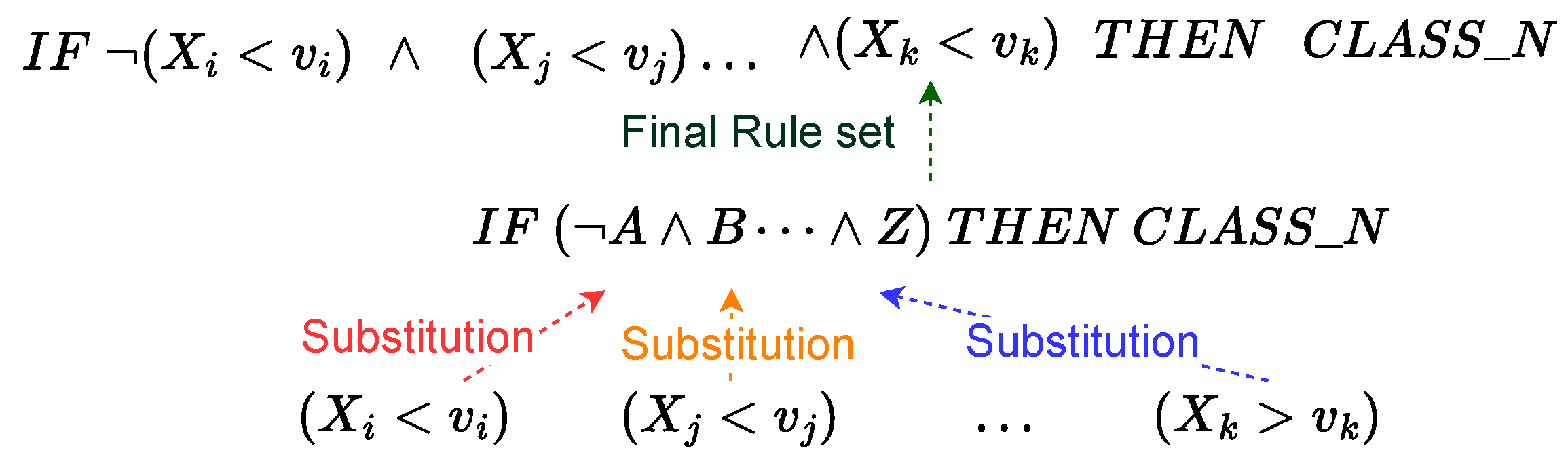
S8: 

Final rule set generation: Per class, intermediate rule sets are merged with the initial_rule_set to produce the final_rule_set (Algorithm 1 line 26). In this step, Hypotheses 3 and 4 are tested. The substitution process carried out to produce the final rule set can be visualized in Figure 6.

S9: 

Final rule-set evaluation: Once the final rule set has been generated, its predictions ${\widehat{\mathbf{y}}}_{rs}$ are evaluated against the true labels ($\mathbf{y}$) predictions ($\widehat{\mathbf{y}}$) to measure rule accuracy and fidelity (Algorithm 1 lines 28 and 30).

4. Experimental Setup

This section elaborates on the experimental setup, datasets used for the evaluation, and experimental process adopted to verify the hypotheses outlined in Section 3. Figure 7 shows the experimental workflow. A detailed description of each experimental step (ES) follows.

4.1. ES1 Scenario Definition

Recalling that DEXiRE is a decompositional rule-extraction method designed to extract rules from DL classifiers, its features’ rule generation (step S7 of the pipeline) operates differently for binary and multiclass classification. On the one hand, for binary classification (SC1), S7 consists of learning the initial rule set (the rule set between the input features and the first hidden layer) using explainable layers (ExpL). ExpL is an additional layer added to the original mode that can learn the activation threshold that splits the decision region between two classes [60]. On the other hand, multiclass classification (SC2) concerns three or more target categories. In the case of SC2, S7 employs algorithms like ID3, C4.5, and OneR to induce the initial rule set for each class.

4.2. ES2 Datasets Gathering

For this study, we selected publicly accessible datasets. Public datasets foster the replication and extension of our study. In particular, the datasets we employed are:

• SC1 Binary classification datasets:

  -

  Breast Cancer Wisconsin (Diagnosis): The Breast Cancer Wisconsin Diagnosis (BCWD) dataset is a binary classification tabular dataset with 30 features and 569 instances. The BCWD dataset includes annotations to determine if a given data instance describes a malign (M) or benign (B) breast tumor [66]. A detailed description of features can be found in Appendix A.1.

  -

  Banknote authentication Dataset The banknote dataset is a binary classification tabular dataset with 1372 instances and four continuous features extracted from the instances’ image wavelet transform. In addition, the banknote dataset includes annotations to classify a banknote as authentic or fake [67]. A detailed description of features can be found in Appendix A.2.

  -

  Prima Indians diabetes mellitus classification The Prima Indians diabetes dataset is a binary classification tabular dataset that contains 768 instances (patients) and eight features. The Prima Indians diabetes dataset includes annotations to determine if a given patient is diabetic or not [68]. A detailed description of features can be found in Appendix A.3.

• SC2 Multiclass classification datasets:

  -

  Digits Dataset: The Digits dataset is a multiclass classification tabular dataset with 1797 instances and 64 features, each one representing the intensity of a gray-scale pixel. The Digits dataset provides annotations to classify digits between 0 and 9 [67]. A detailed description of features can be found in Appendix A.4.

  -

  Iris: The Iris dataset is a popular multiclass classification tabular dataset that contains 150 instances and four features (petal length, sepal length, petal width, and sepal width). The Iris dataset provides annotations to classify an instance between one of three target categories (Setosa, Virginica, Versicolor). A detailed description of features can be found in Appendix A.5.

  -

  Wine quality: The wine quality dataset is a multiclass classification tabular dataset with 178 instances and 13 numeric features. The wine quality dataset provides annotations to classify wine into one of three classes [67]. A detailed description of features can be found in Appendix A.6.

4.3. ES3 Datasets Pre-Processing

Data normalization has been the first step in the pre-processing pipeline. Normalization changes the scale and range of data to improve the training process and reduce the bias induced by the feature ranges. In this study, all features have been normalized using the Z-score normalization. The one-hot encoding procedure transforms the target labels (y) into binary vectors.

Once the dataset has been normalized and the labels encoded, the dataset is separated into three sets: training set (60%), validation set (20%), and test set (20%) using stratified sampling and a random seed of 42.

4.4. ES4 Baseline Predictor Characterization

In ES4, the baseline DL predictor is defined. The baseline DL predictor is a feed-forward DL model, and its architecture is defined for each dataset based on the number and type of features and labels. In turn, it is trained using the training and validation sets as described in experimental step ES3 (Section 4.3). The trained baseline predictor is evaluated using the test set and the performance metrics on the task in order to check the generalization ability and establish the baseline measure. The performance metrics used in this study are accuracy-score for binary classification and F1-score with micro-average for the multiclass task.

4.5. ES5 DEXiRE Application

In ES5, DEXiRE is applied to extract rules from the DL predictor (see Algorithm 1, lines 11 to 28). In turn, the obtained final rule set is evaluated with the test set and predictions from the DL predictor (see Algorithm 1 lines 28 to 30), employing accuracy-score for scenario S1 and F1-score with micro-average in scenario S2. All experiments were executed on a laptop with Intel Core i7, 32 GB of RAM, and Windows 10. The software requirements to replicate the study are python (v3.7), TensorFlow (v2.3.0), Larq (v0.12.2).

5. Results

In this section, experimental results are presented, discriminated by scenario (scenario SC1 and scenario SC2), as was described in Section 4.1.

5.1. SC1 Binary Classification

Results per dataset are shown in

Table 1. Summary table Scenario SC1 (binary classification) showing results for rule-extraction approach, accuracy, fidelity, rule length, and execution time for each dataset. Numerical results are reported with average value ± standard deviation. The best results in each dataset are shown in bold.

Dataset	Approach	Accuracy	Fidelity	Rule Length	Execution Time
BCWD	DL predictor	$0.97\pm 0.010$	NA	NA	NA
	ECLAIRE	$\mathbf{0}.\mathbf{93}\pm \mathbf{0}.\mathbf{004}$	$\mathbf{0}.\mathbf{93}\pm \mathbf{0}.\mathbf{015}$	$6.4\pm 3.2$	$471\mathrm{ms}\pm 18.3\mathrm{ms}$
	DEXiRE	$0.89\pm 0.013$	$0.90\pm 0.013$	$\mathbf{4}.\mathbf{8}\pm \mathbf{2}.\mathbf{0}$	$\mathbf{178}\mathbf{ms}\pm \mathbf{1}.\mathbf{2}\mathbf{ms}$
Banknote	DL predictor	$0.98\pm 0.008$	NA	NA	NA
	ECLAIRE	$0.94\pm 0.036$	$0.95\pm 0.026$	$13.8\pm 0.4$	$213\mathrm{ms}\pm 3.08\mathrm{ms}$
	DEXiRE	$\mathbf{0}.\mathbf{94}\pm \mathbf{0}.\mathbf{032}$	$\mathbf{0}.\mathbf{95}\pm \mathbf{0}.\mathbf{026}$	$\mathbf{13}.\mathbf{8}\pm \mathbf{0}.\mathbf{4}$	$\mathbf{212}\mathbf{ms}\pm \mathbf{2}.\mathbf{17}\mathbf{ms}$
Prima diabetes	DL predictor	$0.76\pm 0.017$	NA	NA	NA
	ECLAIRE	$0.73\pm 0.025$	$0.86\pm 0.031$	$11.8\pm 5.1$	$381\mathrm{ms}\pm 7.56\mathrm{ms}$
	DEXiRE	$\mathbf{0}.\mathbf{75}\pm \mathbf{0}.\mathbf{027}$	$\mathbf{0}.\mathbf{90}\pm \mathbf{0}.\mathbf{018}$	$\mathbf{8}.\mathbf{4}\pm \mathbf{1}.\mathbf{9}$	$\mathbf{232}\mathbf{ms}\pm \mathbf{3}.\mathbf{37}\mathbf{ms}$

. Results are obtained by applying the experimental setup described in Section 4 to three publicly available datasets. The initial model to be explained is a DL predictor ($F_{\mathrm{\Theta }}$) without binarization, and it is used as input for both rule-extraction algorithms ECLAIRE and DEXiRE. The initial DL predictor ($F_{\mathrm{\Theta }}$) was trained and tested using five-fold cross-validation. The accuracy result reported for each DL predictor without binarization is the average accuracy-score measured on each fold.

Scenario (SC1) was tested on three publicly available datasets. Datasets employed in this scenario were briefly described in Section 4.2. The first column in Table 1 identifies the dataset. For each dataset, the second column describes the approach employed to extract rules from the DL predictor ($f_{\mathrm{\Theta }}$). In this scenario, two rule-extraction algorithms were tested, ECLAIRE and DEXiRE. ECLAIRE is the current state-of-the-art algorithm for rule extraction [19] and the baseline method for rule extraction. DEXiRE is our proposed approach for rule extraction, described in further detail in Section 3.

The third column presents the average accuracy-score for ECLAIRE and DEXiRE on the test set. The fourth column describes the fidelity measure, which quantifies the similarity between the DL model’s predictions and those from the extracted rule sets (Definition 5). The fifth column describes the average rule length (the number of terms on each rule set, Definition 7) resulting from five-fold cross-validation. Finally, the sixth column presents the average and standard deviation of the rule-extraction algorithms’ execution time, calculated based on the time measured on 100 executions using the same model and train set.

The Breast Cancer Wisconsin Diagnosis (BCWD) dataset is the first dataset shown in Table 1. BCWD dataset consists of 30 features and two target classes (for a detailed description of this dataset, see Appendix A.1). The DL predictor’s accuracy is 97% with a standard deviation of (≈1%), which shows a consistent performance of this model. The rule sets generated by ECLAIRE have an average accuracy of 93% with a standard deviation of (≈0.4%), whereas the rule sets generated by DEXiRE have an average accuracy of 89% with a standard deviation of (≈1.3%). Example rule sets extracted from the DL predictor are presented in Appendix B.1. ECLAIRE’s example rule set is shown in

Table A9. Final rule set, for the BCWD dataset generated by ECLAIRE.

Rules
$IF\left[\right(perimeter\_worst\le 0.2355\left)\right]\vee \left[\right(concave\_points\_worst\le 0.388\left)\right]THENBenign$
$IF\left[\right(concave\_points\_worst>0.388\left)\right]\vee \left[\right(perimeter\_worst>0.2355\left)\right]THENMalign$

and consists of four terms. Features employed in this rule set were $concave\_points\_worst$ and $perimeter\_worst$. Similarly, the example rule set produced by DEXiRE (

Table A8. Final rule set, for the BCWD dataset generated by DEXiRE.

Rules
$IF\left[\right(concave\_points\_worst>0.388\left)\right]\vee \left[\right(perimeter\_mean>0.4003\left)\right]THENMalign$
$IF\left[\right(concave\_points\_worst\le 0.388)\wedge (perimeter\_mean\le 0.4003\left)\right]THENBenign$

) consists of four terms.

The second dataset shown in Table 1 is the Banknote authentication dataset. The banknote dataset consists of four features, taken from wavelet transform applied to banknote images, and two target classes to decide whether a banknote is authentic. A detailed description of this dataset can be found in Appendix A.2. For this dataset, the DL predictor’s accuracy is 98% with a standard deviation of $0.08\%$. The accuracy measure for ECLAIRE’s rule set was, on average 94% with a standard deviation of $3.6\%$. Similarly, DEXiRE’s rule set presents an average accuracy of 94% and a standard deviation of $3.2\%$. The accuracy difference between the DL predictor and the rule sets varies ≈4%. Meanwhile, ECLAIRE’s and DEXiRE’s rule sets have a fidelity score of 95% with a standard deviation of $2.6\%$. Execution time is comparable in both datasets. Examples of the extracted rule sets from the DL predictor are presented in Appendix B.2. An example of ECLAIRE’s rule set for the banknote dataset is shown in

Table A12. Final rule set for the Banknote authentication dataset generated by ECLAIRE.

Rules
$$\begin{gathered} IF\left[\right(Kurtosis\_of\_Wavelet\_Transformed\_image>1.2494)\wedge \\ (Variance\_of\_Wavelet\_Transformed\_image>-0.7811\left)\right]\vee \\ \left[\right(Variance\_of\_Wavelet\_Transformed\_image>0.1144\left)\right]\vee \\ \left[\right(Skewness\_of\_Wavelet\_Transformed\_image>0.5262)\wedge \\ (Variance\_of\_Wavelet\_Transformed\_image>-1.0579\left)\right]THEN0 \end{gathered}$$
$$\begin{gathered} IF\left[\right(Kurtosis\_of\_Wavelet\_Transformed\_image\le 1.2494)\wedge \\ (Skewness\_of\_Wavelet\_Transformed\_image\le 0.5262)\wedge \\ (Variance\_of\_Wavelet\_Transformed\_image\le 0.1144\left)\right]\vee \\ \left[\right(Variance\_of\_Wavelet\_Transformed\_image\le -1.0579\left)\right]\vee \\ \left[\right(Skewness\_of\_Wavelet\_Transformed\_image\le 0.5262)\wedge \\ (Variance\_of\_Wavelet\_Transformed\_image\le -0.7811\left)\right]THEN1 \end{gathered}$$

. An example of DEXiRE’s rule set is shown in

Table A11. Final rule set, for the banknote authentication dataset generated by DEXiRE.

Rule
$$\begin{gathered} IF\left[\right(Kurtosis\_of\_Wavelet\_Transformed\_image>0.3402)\wedge \\ (Skewness\_of\_Wavelet\_Transformed\_image>-0.6451\left)\right]\vee \\ \left[\right(Skewness\_of\_Wavelet\_Transformed\_image>0.486)\wedge \\ (Variance\_of\_Wavelet\_Transformed\_image>-1.0579\left)\right]\vee \\ \left[\right(Skewness\_of\_Wavelet\_Transformed\_image>0.328)\wedge \\ (Variance\_of\_Wavelet\_Transformed\_image>0.1144\left)\right]\vee \\ \left[\right(Kurtosis\_of\_Wavelet\_Transformed\_image>-0.7389)\wedge \\ (Variance\_of\_Wavelet\_Transformed\_image>0.1144\left)\right]THEN0 \end{gathered}$$
$$\begin{gathered} IF\left[\right(Kurtosis\_of\_Wavelet\_Transformed\_image\le -0.7389)\wedge \\ (Skewness\_of\_Wavelet\_Transformed\_image\le 0.328\left)\right]\vee \\ \left[\right(Variance\_of\_Wavelet\_Transformed\_image\le -1.0579\left)\right]\vee \\ \left[\right(Skewness\_of\_Wavelet\_Transformed\_image\le -0.6451)\wedge \\ (Variance\_of\_Wavelet\_Transformed\_image\le 0.1144\left)\right]\vee \\ \left[\right(Kurtosis\_of\_Wavelet\_Transformed\_image\le 0.3402)\wedge \\ (Skewness\_of\_Wavelet\_Transformed\_image\le 0.486)\wedge \\ (Variance\_of\_Wavelet\_Transformed\_image\le 0.1144\left)\right]THEN1 \end{gathered}$$

. ECLAIRE’s rule set example consists of 10 terms, whereas DEXiRE’s consists of 14 terms. Both rule sets exclude the feature $entropy\_of\_image$.

The Prima Indian Diabetes dataset results are shown at the bottom of Table 1. The Prima diabetes dataset consists of eight features obtained from female patients and two target classes to classify a patient as diabetic or non-diabetic. A detailed description of this dataset can be found in Appendix A.3. The DL predictor’s accuracy is 76% with a standard deviation of $1.7\%$. ECLAIRE’s rule set has an average accuracy of $73\%$ with a standard deviation of $2.5\%$, and DEXiRE’s rule set reports an average accuracy of $75\%$ with a standard deviation of $2.7\%$. The accuracy variation between the baseline and the rule sets is ≈3%. ECLAIRE’s rule set has a fidelity score of 86% with a standard deviation of $3.1\%$. DEXiRE’s rule set has a fidelity score of 90% with a standard deviation of $1.8\%$. Example rule sets extracted from the DL predictor are presented in Appendix B.3. An example of ECLAIRE’s rule set is shown in

Table A15. Final rule set for the Prima Diabetes dataset generated by ECLAIRE.

Rules
$IF\left[\right(Glucose>0.6918\left)\right]\vee \left[\right(Pregnancies>0.343)\wedge (SkinThickness>0.7191\left)\right]\vee \left[\right(BMI>0.7878\left)\right(Glucose>-0.028\left)\right]\vee \left[\right(BMI>0.4832)\wedge (Glucose>-0.1219\left)\right]\vee \left[\right(Glucose>0.7857\left)\right]\vee \left[\right(BMI>-0.2021)\wedge (Glucose>0.6605\left)\right]THEN1$
$IF\left[\right(BMI\le 0.0898\left)\right]\vee \left[\right(Glucose\le 0.0346)\wedge (SkinThickness\le 1.0327\left)\right]\vee \left[\right(Glucose\le -0.1532\left)\right]\vee \left[\right(Glucose\le -0.1219)\wedge (Pregnancies\le 0.6399\left)\right]\vee \left[\right(BMI\le 0.3309)\wedge (Glucose\le 0.1598\left)\right]\vee \left[\right(Glucose\le 0.0659\left)AND\right(SkinThickness\le 0.5936\left)\right]\vee \left[\right(BMI\le -0.2656\left)AND\right(Glucose\le 0.3476)\wedge (SkinThickness\le 0.5936\left)\right]THEN0$

consists of 22 terms, whereas an example of DEXiRE’s rule set is shown in

Table A14. Final rule set, for the Prima Indians diabetes dataset, generated by DEXiRE.

Rule
$IF\left[\right(BMI>0.8576)\wedge (Glucose\le -0.341\left)\right]\vee \left[\right(BMI\le -0.2212)\wedge (Glucose>0.2067)\wedge (Pregnancies\le -0.1025\left)\right]\vee \left[\right(BMI\le 0.8576)\wedge (Glucose\le 0.2067\left)\right]THEN0$
$IF\left[\right(BMI\le -0.2212)\wedge (Glucose>0.2067)\wedge (Pregnancies>-0.1025\left)\right]\vee \left[\right(BMI>0.8576)\wedge (Glucose\le 0.2067)\wedge (Glucose>-0.341\left)\right]\vee \left[\right(BMI>-0.2212)\wedge (Glucose>0.2067\left)\right]THEN1$

and consists of 10 terms. DEXiRE’s rule set example employs features: BMI, glucose, and pregnancies, whereas ECLAIRE’s rule set uses the same features with the addition of $SkinThickness$.

5.2. SC2 Multiclass Classification

Scenario (SC2) is devoted to a multiclass task and was tested on three datasets. Scenario SC2 differs from scenario SC1 in the technique employed to induce the features’ rule sets. While SC1 uses ExpL, SC2 employs a decision tree as a rule inductor. Datasets tested in this scenario are briefly described in Section 4.2. The first column in

Table 2. Summary table Scenario SC2 (multiclass classification) showing results for Rule extraction approach, Accuracy, fidelity, rule length, and execution time for each dataset. Numerical results are reported with average value ± standard deviation. The best results in each dataset are shown in bold.

Dataset	Approach	Accuracy	Fidelity	Rule Length	Execution Time
Digits	DL predictor	$0.96\pm 0.010$	NA	NA	NA
	ECLAIRE	$\mathbf{0}.\mathbf{82}\pm \mathbf{0}.\mathbf{010}$	$\mathbf{0}.\mathbf{81}\pm \mathbf{0}.\mathbf{010}$	$81.0\pm 8.1$	$9200\mathrm{ms}\pm 124\mathrm{ms}$
	DEXiRE (Th = 60%)	$0.44\pm 0.149$	$0.43\pm 0.147$	$\mathbf{37}.\mathbf{6}\pm \mathbf{3}.\mathbf{0}$	$\mathbf{442}\mathbf{ms}\pm \mathbf{5}.\mathbf{3}\mathbf{ms}$
	DEXiRE (Th = 50%)	$0.50\pm 0.163$	$0.50\pm 0.167$	$39.0\pm 2.6$	$481\mathrm{ms}\pm 8.74\mathrm{ms}$
	DEXiRE (Th = 25%)	$0.79\pm 0.025$	$0.79\pm 0.020$	$44.8\pm 1.0$	$490\mathrm{ms}\pm 6.94\mathrm{ms}$
Iris	DL predictor	$0.93\pm 0.057$	NA	NA	NA
	ECLAIRE	$0.89\pm 0.083$	$0.89\pm 0.039$	$5.6\pm 1.0$	$177\mathrm{ms}\pm 2.19\mathrm{ms}$
	DEXiRE	$\mathbf{0}.\mathbf{90}\pm \mathbf{0}.\mathbf{059}$	$\mathbf{0}.\mathbf{95}\pm \mathbf{0}.\mathbf{026}$	$\mathbf{4}.\mathbf{0}\pm \mathbf{0}.\mathbf{0}$	$\mathbf{0}.\mathbf{916}\mathbf{ms}\pm \mathbf{0}.\mathbf{002}\mathbf{ms}$
Wine quality	DL predictor	$0.99\pm 0.014$	NA	NA	NA
	ECLAIRE	$0.83\pm 0.073$	$0.84\pm 0.084$	$\mathbf{3}.\mathbf{2}\pm \mathbf{0}.\mathbf{4}$	$249\mathrm{ms}\pm 5.84\mathrm{ms}$
	DEXiRE	$\mathbf{0}.\mathbf{87}\pm \mathbf{0}.\mathbf{028}$	$\mathbf{0}.\mathbf{87}\pm \mathbf{0}.\mathbf{028}$	$4.0\pm 0.0$	$\mathbf{209}\mathbf{ms}\pm \mathbf{1}.\mathbf{05}\mathbf{ms}$

identifies the dataset. For each dataset, the second column on Table 2 lists the approach employed to extract rules from the baseline predictor ($f_{\mathrm{\Theta }}$). The third column presents the average accuracy for each approach measured on the test set, calculated as the average value of five-fold cross-validation training. The fourth column describes the fidelity measure (Definition 5), which quantifies the similarity between the DL model’s predictions and those from the extracted rule sets. The fifth column describes the average rule length (the number of terms on each rule set, Definition 7) calculated as the average rule length in the rule set per fold in five-fold cross-validation. Finally, the last column presents the average and standard deviation of the rule-extraction algorithms’ execution time, calculated as the average time of 100 executions employing a fixed DL predictor and train set.

The Digits dataset shown at the top of Table 2, which consists of 64 features and ten target classes (digits from 0 to 9). A detailed description of this dataset can be found in Appendix A.4). The DL predictor’s accuracy is 96% with a standard deviation of $1\%$. The rule sets extracted with ECLAIRE have an accuracy of $82\%$ with a standard deviation of $1\%$. The coverage threshold (Th) is a parameter that filters out those terms with low coverage levels reducing the rule sets’ length. To evaluate the impact of coverage threshold (Th) on the accuracy, fidelity, rule length, and execution time, DEXiRE was tested on different coverage threshold levels. The first row in Table 2 shows DEXiRE results for different Th (60%, 50%, 25%) levels. The default Th value for DEXiRE is 60%; for this Th value, DEXIRE’s rule sets obtained an average accuracy of 44% with a standard deviation of $1.49\%$. For a Th value of 50%, the average accuracy obtained is 50% with a standard deviation of $1.63\%$. Finally, for a Th value of 25%, the average accuracy obtained is 79%, with a standard deviation of $2.5\%$. Fidelity follows a similar behavior. For the Th value of $60\%$, the obtained average fidelity of $43\%$ with a standard deviation of $1.47\%$. For the Th value of $50\%$, the average fidelity value is $50\%$ with a standard deviation of $1.67\%$, and finally, for the Th value of $25\%$, the obtained average fidelity is $79\%$ with a standard deviation of $2\%$.

The Iris dataset consists of four features, taken from flowers’ petals and sepals width and length, with three target classes (Setosa, Virginica, and Versicolor) (Appendix A.5). Performance measures for the Iris dataset are shown in the middle of Table 2. The DL predictor’s accuracy is 92% with a standard deviation of $5.7\%$. The average accuracy for ECLAIRE’s rule sets is $89\%$ with a standard deviation of $8.3\%$, while DEXiRE’s rule sets obtained an average accuracy value of 90% with a standard deviation of $5.9\%$. ECLAIRE’s rule set has obtained an average fidelity value of 89% with a standard deviation of $3.9\%$. For DEXiRE, the rule sets have obtained an average fidelity value of 90% with a standard deviation of $5.9\%$. Rule sets examples extracted from the DL predictor are presented in Appendix B.5. An example of ECLAIRE’s rule sets is shown in

Table A19. Final rule set for the Iris dataset generated by ECLAIRE.

Rules
$IF\left[\right(petal\_width\_\left(cm\right)\le 0.6518)\wedge (sepal\_width\_\left(cm\right)\le -0.1082\left)\right]THEN1$
$IF\left[\right(petal\_width\_\left(cm\right)>0.3884\left)\right]THEN2$
$IF\left[\right(petal\_width\_\left(cm\right)\le -0.7966\left)\right]THEN0$

and consists of six terms, whereas an example DEXiRE’s rule set is shown in

Table A18. Final rule set for the Iris dataset generated by DEXiRE.

Rules
$IF\left[\right(petal\_length\_\left(cm\right)>0.4713\left)\right]THEN2$
$IF\left[\right(petal\_length\_\left(cm\right)\le 0.4713\left)AND\right(petal\_length\_\left(cm\right)>-1.0618\left)\right]THEN1$
$IF\left[\right(petal\_length\_\left(cm\right)\le -1.0618\left)\right]THEN0$

consists of four terms. ECLAIRE’s rule set example includes $sepal\_width$ and $petal\_width$ whereas DEXiRE’s rule set only employs pedal features ($petal\_width$ and $petal\_lenght$).

The Wine quality dataset is the third last dataset shown at the bottom of Table 2. The Wine quality dataset comprises 13 features that describe factors affecting the wine’s quality and taste. The target category is one of three classes of wine, a detailed description of this dataset can be found in Appendix A.6. The DL predictor’s accuracy is 99% with a standard deviation of $1.4\%$. The average accuracy value for ECLAIRE’s rule sets is 83% with a standard deviation of $7.3\%$. The DEXiRE’s rule sets have obtained an average accuracy value of 87% with a standard deviation of $2.8\%$. The accuracy variation between the DL predictor and the rule sets is ≈17%. ECLAIRE’s rule sets have an average fidelity value of 84% with a standard deviation of $8.4\%$. DEXiRE’s rule sets have an average fidelity value of 87% with a standard deviation of $2.8\%$. Examples of rule sets extracted from the DL predictor are presented in Appendix B.6. An example of ECLAIRE’s rule set is shown in

Table A21. Final rule set for the wine quality dataset generated by ECLAIRE.

Rules
$IF\left[\right(od280/od315\_of\_diluted\_wines\le -0.7086\left)\right]THEN2$
$IF\left[\right(proline>0.2806\left)\right]\vee \left[\right(proline>0.8538\left)\right]THEN0$
$IF\left[\right(color\_intensity\le -0.4837\left)\right]\vee \left[\right(color\_intensity\le -0.1636)\wedge (magnesium\le -0.6138\left)\right]THEN1$

consists of six terms, whereas DEXiRE’s rule set example is shown in

Table A20. Final rule set for the wine quality dataset generated by DEXiRE.

Rules
$IF\left[\right(hue\le -0.2959)\wedge (proline\le 0.6054\left)\right]THEN2$
$IF\left[\right(hue>-0.2959)\wedge (proline\le 0.6054\left)\right]THEN1$
$IF\left[\right(proline>0.6054\left)\right]THEN0$

, and consists of four terms. Both rule sets include the feature $proline$, $color\_intensity$, and $magnesiumfeatures$.

6. Analysis and Discussion

This section elaborates on the obtained results and discusses the points characterizing DEXiRE and its results.

6.1. Analysis Scenario (SC1)

It is worth recalling that the length of the rules refers to the number of Boolean terms composing a rule set (see Definition 7). The average rule length obtained by DEXiRE in scenario SC1 is reported in Table 1 column 4. Looking at it closely, it is possible to notice that for BCWD and Prima Indians diabetes datasets, the average rule length for DEXiRE’s rule sets is 4.8 and 8.4, respectively. Both results are shorter than those obtained by ECLAIRE (6.4 and 11.8, respectively). The DEXiRE and ECLAIRE’s average rule lengths for the banknote dataset are mostly similar, with a value of 13.8.

On the one hand, rule length overlaps can be due to the influence of the dataset characteristics and model internal structure (see Section 6.3.1). On the other hand, the difference (if any) in the average rule length relies on the DEXiRE’s use of binarized hidden layers, explainable layers, and related activation patterns. Differently, ECLAIRE uses continuous activations and decision trees to induce the features and intermediate rule sets. DEXiRE and ECLAIRE reach the same objective (generate a rule from a DL predictor) with different approaches—yet obtain comparable performance. For example, from an accuracy/fidelity point of view, DEXiRE sensibly outperforms ECLAIRE on the Prima Indians diabetes dataset, it equates ECLAIRE w.r.t. in the banknote dataset, and it sensibly underperforms w.r.t. BCWD (see Table 1—columns 3 and 4). However, concerning the execution time, DEXiRE outperforms ECLAIRE ($90\%$ faster in the best-case scenario—BCWD, $48\%$ w.r.t. the Prima Indianas dataset) and mostly identical w.r.t. the banknote dataset.

Although the results obtained by DEXiRE and ECLAIRE are comparable, DEXiRE is able to provide additional insights about the internal decision process carried out by the neurons in the DL predictor (i.e., identify those neurons and their output values highly related with the predicted output). This benefit is provided due to the binarization process and activation pattern generated per class within DEXiRE.

6.2. Analysis Scenario (SC2)

Table 2 column 4 shows the average rule length obtained by DEXiRE in the scenario SC2.

It is worth recalling that DEXiRE employs a coverage threshold that allows to control the number of terms in each rule set (intermediate and final) by setting a minimum coverage threshold (Th) percentage and filtering all the rules with coverage (Definition 6) below the threshold. In the digits dataset, the rule length is $73\%$ shorter than the one produced by ECLAIRE. However, the accuracy and fidelity obtained by DEXiRE are very poor. To achieve the performance obtained by ECLAIRE, we have decreased the Th value. In particular, with a Th value of 25%, accuracy and fidelity are $3\%$ and $2\%$ away from matching the ECLAIRE’s performance while improving on the average rule length, which is 57% shorter than the for ECLAIRE.

In the case of the Iris dataset, the average rule length obtained by DEXiRE is $33\%$ shorter than the one obtained by ECLAIRE. Whereas in the case of the wine quality dataset, the ECLARE’s average rule length is sensibly shorter than the one from DEXiRE. The difference (if any) in the average rule length depends on two main factors: (i) the interrelation between the dataset characteristics and the DL predictor’s internal structure and (ii) the differences in rule-extraction algorithms’ approaches. While DEXiRE employs binarized hidden layers and related activation patterns to extract rules, ECLAIRE uses continuous activations and decision trees to induce the features and intermediate and final rule sets.

Another benefit to DEXiRE’s approach is SEEN in the overall execution time. DEXiRE outperforms ECLAIRE in all datasets ($197\%$ faster in the best-case scenario – Iris dataset, $17\%$ w.r.t the wine quality dataset). Additionally, in this scenario, the standard deviation of the execution time is low for DEXIRE (never exceeding 9 ms). Low variance levels are due to the use of the activation pattern to identify the most relevant neurons in each hidden layer, thus reducing the time for the generation of the intermediate datasets.

In this scenario, DEXiRE and ECLAIRE exhibit comparable results in terms of accuracy and fidelity. While DEXiRE indicates a tendency to produce shorter rule sets and execution times due to the binarization process and activation pattern generated per class, DEXiRE is able to provide additional insights about the internal decision process carried out by the neurons in the DL predictor and filter out those neurons that are not relevant to the decision process carried out by the DL predictor.

6.3. Discussion

This section discusses the results obtained w.r.t. the Hypotheses 1–4 initially formulated.

6.3.1. Data and Models Interdependency

DEXiRE can have similar rule sets’ lengths with (partial) overlapping terms with ECLAIRE. Such overlap(s) can occur since, although they use different procedures, both rely on the same inputs (model and the training dataset) to induce the set of rules.

The final rule set(s) are logical formulations containing (the most relevant) data features integrating the intermediate rule sets. Both ECLAIRE and DEXiRE have similar procedures to induce (predict) intermediate rule sets, relying on the data features. DEXiRE can employ one of two methods (ExpL or decision trees) to generate the feature rule set (Step S7 in Section 3). Similarly, ECLAIRE employs decision trees to induce the features’ rule set.

To understand the effect of the input features on the final rule set, let us analyze the case of the BCWD dataset. This dataset has 30 input features. Although the final rule sets generated by ECLAIRE and DEXiRE differ in the number of terms and the composition of rules, most of them contain the feature concave_points_worst. This tendency raises a question: why is the feature concave_points_worst present in the majority of rule sets produced by different rule-extraction algorithms?

To answer this question, we must analyze the behavior of the feature concave_points_worst w.r.t the DL model’s preconditions and the other features in the dataset. Figure 8 shows the feature ranking according to variance per class w.r.t. DL predictor’s labels ($\widehat{y}$). The features in the upper area present lower variance per class and higher information gain value (see Table A8 and Table A9). Thus, there is a high probability that this feature is selected by the rule generation algorithms (ExpL, decision trees) and included in the final rule set.

Finally, we can infer that features with a high discrimination capability have high chances (yet no certainty) of being included in the final rule set, regardless of the rule induction algorithm employed—explaining the (partial) overlapping obtained in some datasets.

Concerning the influence of the DL predictor’s internal structure (architecture, activations, weights) on the final rule set, it is worth noticing that both DEXiRE and ECLAIRE are decompositional rule-extraction algorithms. This implies that they use the DL predictor’s internal structure to induce rules and identify the neurons responsible for the decisions (verifying Hypotheses 1 and 2).

In conclusion, DL predictors and datasets are essential inputs for rule-extraction algorithms. For this reason, their composition and structure profoundly influence the final rule sets. Finally, it is worth highlighting the interdependence between the data and the DL predictors: the latter (being data-driven models) learn from the former, adjusting their structure and parameters to fit the task.

6.3.2. The Role of Binarization

Extracting rules from hidden layers in neural networks is still an open challenge. The hidden layer’s activations are continuous and non-linear, which is an excellent characteristic for learning parameters with the back-propagation algorithm. However, it is more difficult to interpret their output values w.r.t. to the inputs. To solve this challenge, several decompositional rule-extraction algorithms approximate continuous activations through discrete segments to induce rules on each segment [29]. Nevertheless, these approaches have some limitations. For example, they tend to generate long rule sets (with many terms/rules—not human-readable) and require several phases of pruning and re-training. Moreover, most decompositional approaches are limited to one or a predefined number of hidden layers. DEXiRE overcomes these limitations and simplifies the identification of frequent activation patterns (verifying Hypotheses 1–3).

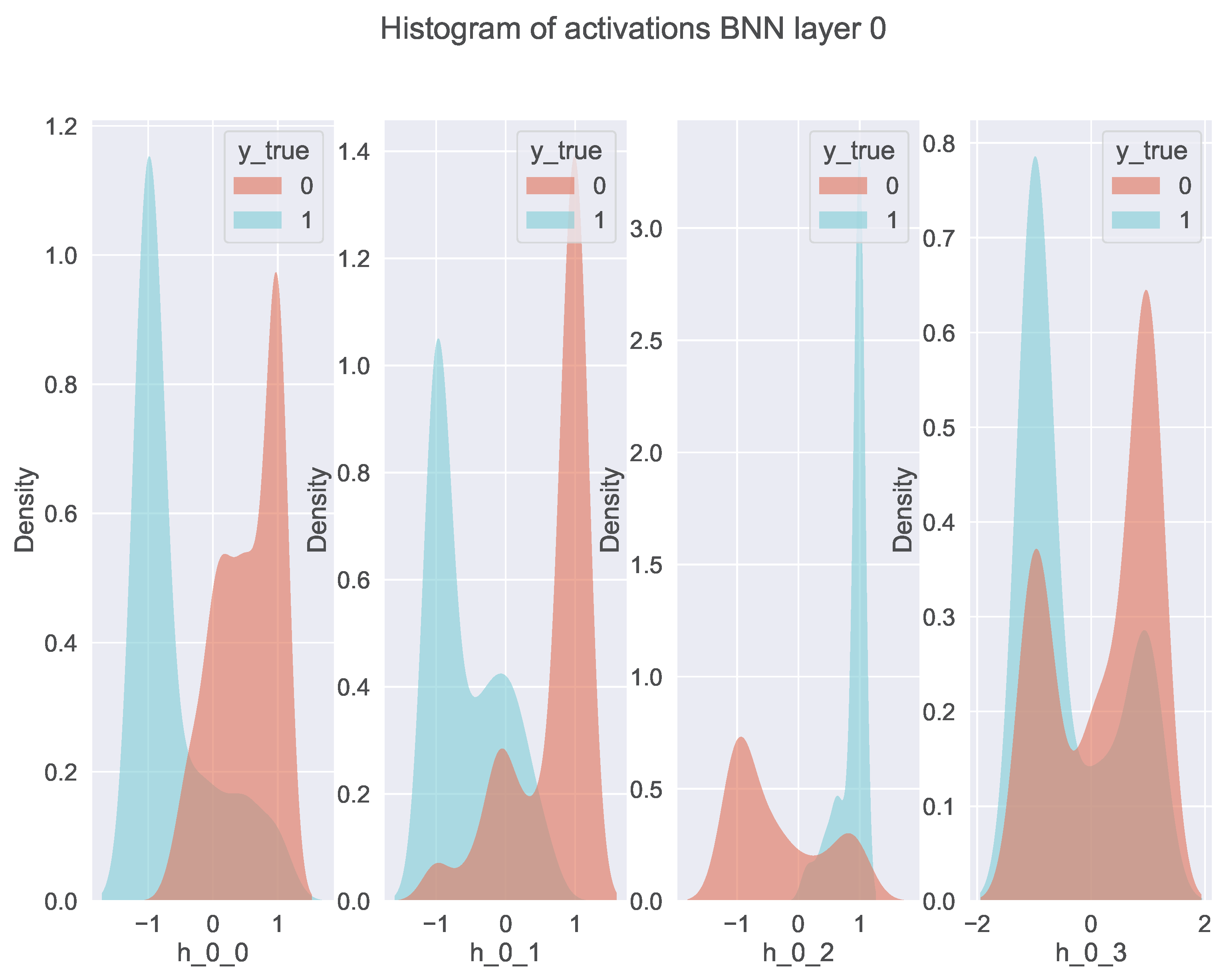
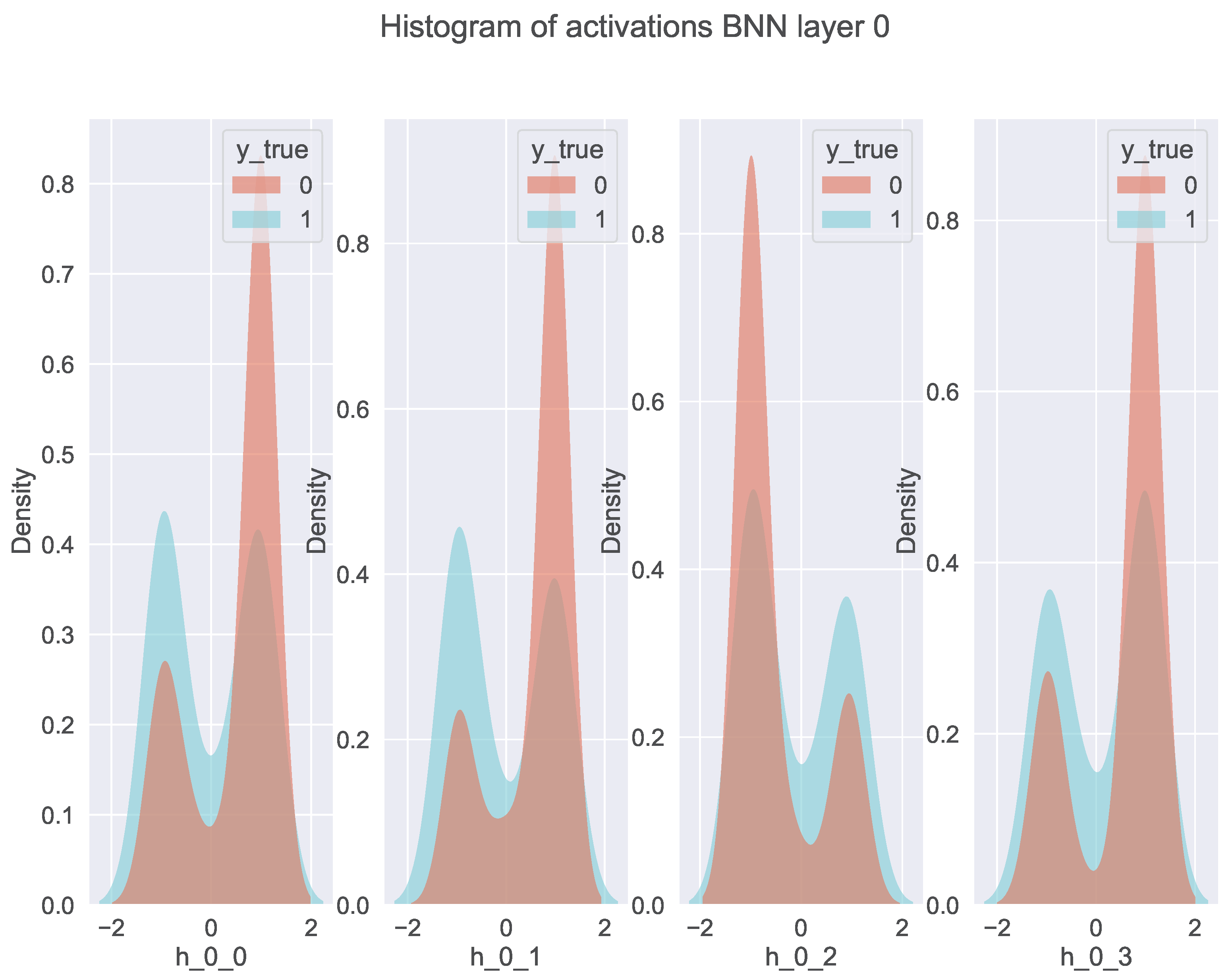
In particular, Hypothesis 1 states that it is possible to identify activation patterns more simply by binarizing the hidden layers of a DL predictor ($f_{\mathrm{\Theta }}$). To test Hypothesis 1, we binarized a trained DL predictor and then extracted the binary activations per hidden layer for each instance in the training set. Finally, using the binary activations, we calculate the kernel density estimation (KDE) for each neuron and visualize it in Figure 9 and Figure 10.

Figure 9 shows the KDE for the first hidden binary layer (hidden layer 0) discriminated by class (class 0 and 1). Moreover, we can observe the high level of polarization present in neurons h_0_0, h_0_7, and h_0_8. Empty plots in this figure indicate neurons with zero variance (the same value for all the instances). Neurons with zero variance do not provide discriminative information, while highly polarized neurons become effective discriminators. Thus, the polarization induced by binary hidden layers and binary neural networks (BNN) allows the identification of activation patterns as described in Algorithm 1.

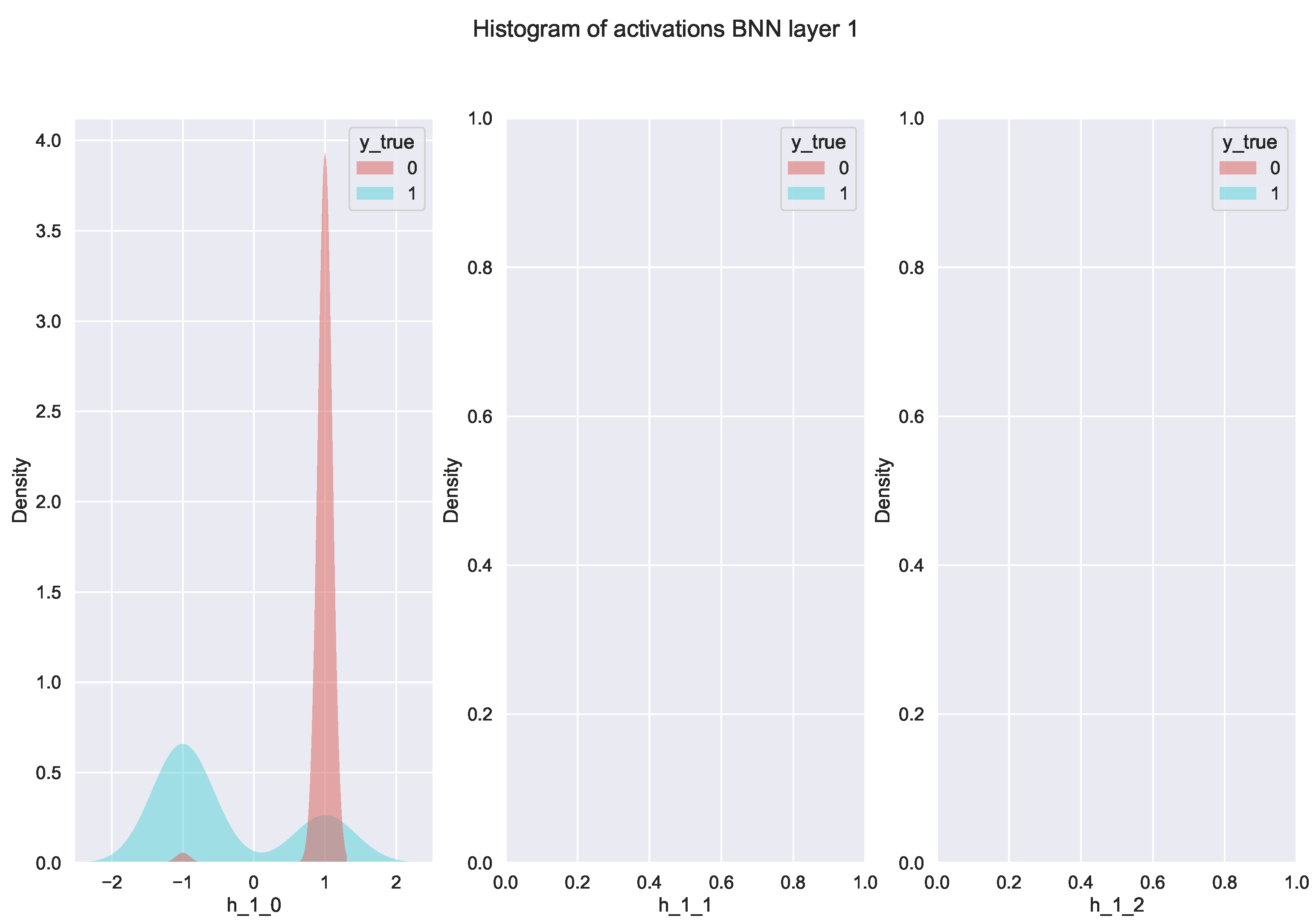
Figure 10 shows the KDE for the second hidden binary layer (hidden layer 1) discriminated by class (class 0 and 1). Similar to the previous layer, we can identify the relevant neurons in the decision of the classifier (neuron h_1_0) and discard those with zero variance. It is worth noticing that the number of discriminative neurons decreases, and the polarization increases as we approach the output layer. Thus, we can consider Hypotheses 2 and 3 validated. Additional KDE analysis for different datasets and DL predictors can be found in Appendix C.

6.3.3. From Neurons to Decisions: Activation Pattern

As was discussed above, binary activations in the hidden layers generate binary patterns representing the input examples transformed by each hidden layer. From those binary patterns, we can filter out those neurons with zero variance because they do not apport discriminative information. With the filtered set of binary patterns, we can identify the most frequently active neurons and their activation values per class, generating an activation pattern.

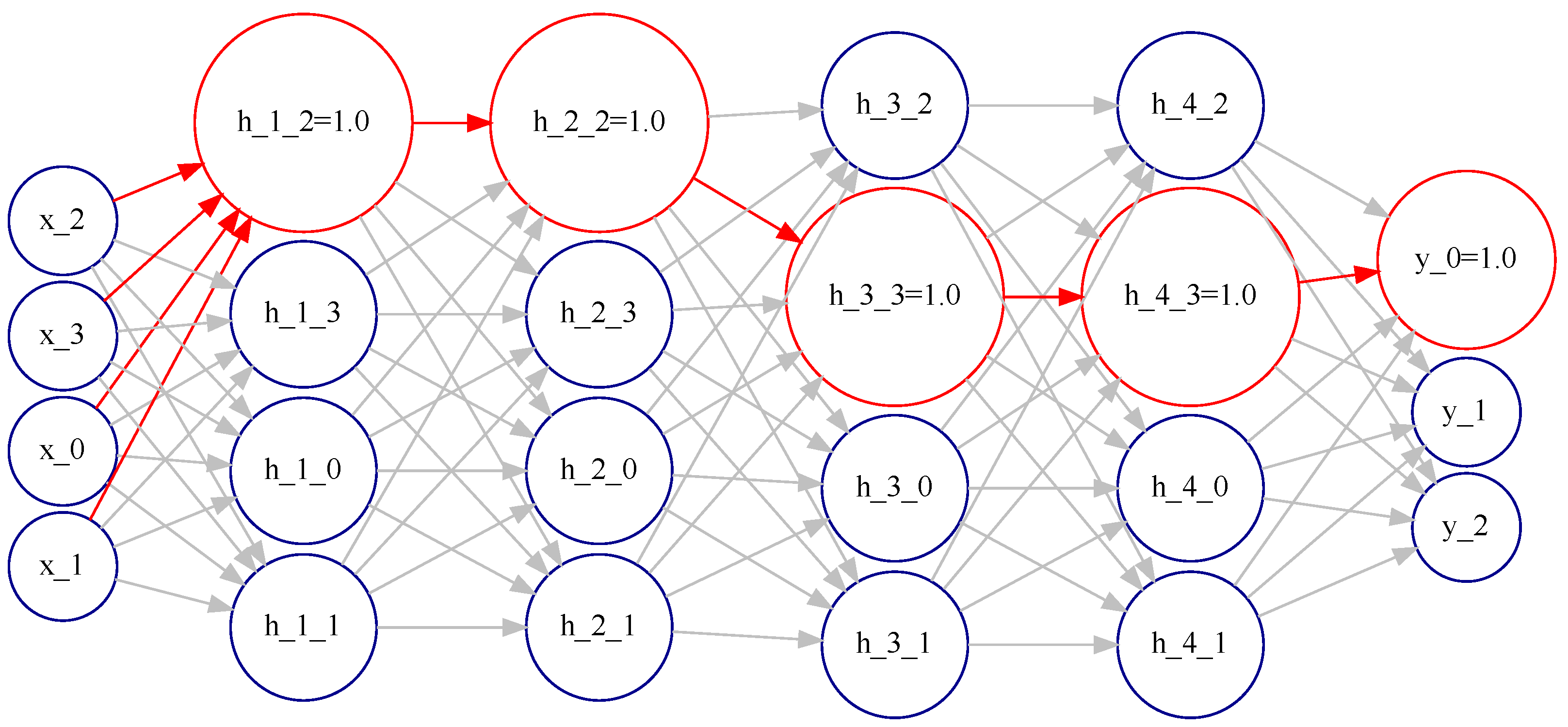
Figure 11 (automatically generated) shows the activation pattern for class 0 in the banknote dataset. The activation pattern is highlighted in red and involves neurons: h_1_0 with activation value $-1$, h_2_0 with activation value 1, and the output neuron y_0_1 with activation value 1. The activation pattern reveals layer by layer the most likely decisions the network is making to reach the final decision.

Figure 12 describes the activation pattern for class 1 in the banknote dataset. The activation pattern is highlighted in red and involves neurons: h_1_1 with activation value 1, h_2_0 with activation value -1, and the output neuron y_1_1 with activation value 1. The activation pattern reveals layer by layer the most likely decisions the network makes to reach the final decision. Comparing the activation pattern for class 0 and class 1, we can gain insight into the internal decision process carried out by the binary DL predictor. For example, we know that decision relies on neurons h_1_0 and h_1_1 for the first hidden layer. For the second hidden layer, the decision is taken by neuron h_2_0, which, acting as a switch, selects the output neuron to activate.

Finally, we can infer that the activation pattern is a valuable explainable artifact that complements the rule sets and provides additional insight into the internal decision process carried out by the binary DL predictor.

6.3.4. Rationales behind Rule Induction

This work employs two methods to induce the feature rules: explainable layers (ExpL) for binary classification tasks (SC1) and decision trees for multiclass classification (SC2).

In scenario SC1, an ExpL is added between the input layer and the first hidden layer. After a fine-tuning training with the rest of the layers frozen, the weights of ExpL codify a threshold value ($v_i$) per feature ($x_i$) that splits the input space in two, indicating the point of maximum information gain per feature. Using the learned threshold values is possible to induce simple rules per feature ($x_i$) in the form of $if(x_i\ge v_i)thenclass1;elseclass0$, combining these simple rules into the intermediate rule set the final rule set is obtained [60]. ExpL layers are suitable for binary classification tasks, given their ability to split the space into binary buckets with complementary rules. Figure 13 shows the density function discriminated by class for the feature variance_of_the_wavelet_transform (class 0 in blue and class 1 in orange), and the learned threshold value ($v_i$) (shown as a vertical red line) that splits the input space for class 0 and 1.

In the multiclass task case, and given its binary rule induction characteristic, ExpL must employ a series of One-vs-Rest setups. However, one-vs-Rest setups imply a high computational cost due to the increasing number of models to train as the number of classes increases. Equation (9) provides the number of models to train in a One-vs-Rest setup. Applying such a formula to a dataset with three target classes, the required number of models to induce the rule set is 3. However, if we extend the target classes to 10 (Digits dataset), the models to train scale to 45. Additionally, ExpL produces binary splits per class (One-vs-Rest), which are not expressive enough to model the complex decision boundaries of multiclass models, producing low-accurate rule sets in the case of the multiclass task. Due to these reasons, in scenario SC2, we have employed as features’ rule inductor the decision trees algorithm (C4.5). Finally, through SC1 and SC2, we have shown that DEXiRE can be applied for both binary and multiclass classification—verifying Hypothesis 4.

$$C_{n_{classes},2}=\frac{n_{classes}!}{2!(n_{classes}-2!)}$$

(9)

6.3.5. Beyond Rule Sets

DEXiRE provides characteristics that go beyond other rule-extraction algorithms. In particular:

• Tuneable threshold rule set granularity: DEXiRE provides a fine granularity control over the number of terms in the intermediate and final rule sets. While algorithms such as ECLAIRE control term expansion indirectly through decision tree parameters, DEXiRE provides fine control over the number of terms and the number of clauses through the coverage threshold (Th) parameter. It filters out terms and clauses with low coverage or those conflicting with other rules with higher coverage or confidence values.
• Understand per class discriminative neurons: As discussed above, using binary activations and identifying the activation pattern allow us to obtain clues about the predictor’s decision process. It is also possible to identify those neurons discriminating by class and their value and concentrate the analysis on them, removing those neurons with zero variance.
• activation pattern supports the knowledge injection: The activation pattern allows identifying the more frequently activated binary neurons per class in each hidden layer along with its activation value. This information helps to describe the DL estimator’s internal decision process, and additionally, the activation pattern can also be used to inject symbolic knowledge within the neural network [69,70,71]. Symbolic artificial intelligence (AI) relies on high-level knowledge usually expressed as rules, logic predicates, or ontologies [22]. On the other hand, subsymbolic AI is data-driven, as in the case of DL predictors. Nevertheless, subsymbolic and symbolic AI paradigms can be combined following the Hypothesis 2, which states that binary neurons behave as a Boolean logic function. Therefore, first-order logic predicates can be embedded into a Boolean function and then integrated as a binary neuron or layer into the binary DL predictor, with the additional advantage that both symbolic and subsymbolic neurons can co-exist and interact in the same network.

6.3.6. Constraints and Limitations

Besides the advantages discussed above, as of today, DEXiRE is still subjected to some constraints (C) and limitations (L):

C:

To identify the activation pattern, DEXiRE requires that the output layer has as many neurons as classes and that the class labels are encoded in one hot encoder.

L:

Currently, DEXiRE has been tested on the classification task (binary and multiclass classification) with comparable results to the state-of-the-art rule extractors. However, DEXiRE needs to be extended to perform additional tasks, such as rule extraction in the regression task and in the multi-labeling task. These additional capabilities are proposed in future work.

L:

To date, DEXiRE can work with a feed-forward neural network (with any number of hidden layers). DEXiRE has not been designed to work with convolutional neural networks (CNN), recurrent neural networks (RNN), or Transformers. However, based on the verified hypotheses, it can also be extended to work with these kinds of DL models.

7. Conclusions and Future Work

This paper presents DEXiRE, a decompositional rule-extraction algorithm based on hidden layers’ binarization, path identification, and layer-by-layer rule induction. DEXiRE has been developed following the Hypotheses 1–4, and it has been tested in two scenarios, binary classification (SC1) and multiclass classification (SC2), with six publicly available datasets.

Attributes and performance of DEXiRE have been compared with ECLAIRE (state-of-the-art for decompositional rule extraction), leading to the conclusion that:

• DEXiRE can be applied to extract rules from DL predictors with any number of hidden layers. The layer-by-layer generated rules do not affect nor depend on rules in other layers. The resulting independence reduces the complexity of the intermediate rule sets and eliminates the limitation of being able to process only one or a fixed predefined number of layers. Indeed, approaches such as FERNN [48] do not scale as they express the rules of a given layer as a function of those from other layers.
• DEXiRE has been tested in binary and multiclass classification scenarios, obtaining performance (accuracy and fidelity) comparable to ECLAIRE.
• Binary neurons with a high degree of polarization in each hidden layer become effective discriminators capable of identifying, through a binary pattern, instances that belong to a particular class. Binary neurons can be expressed as Boolean functions and the relative Boolean intermediate rule sets.
• The activation pattern identifies the most frequently activated binary neurons per class for each layer and filters out irrelevant or redundant neurons. The activation pattern provides additional explainable insights about the DL predictor’s internal decision process and reduces the size of the intermediate rule sets and the execution time.

As the feature work, we envision extending DEXiRE to (i) handle regression tasks, (ii) develop a module for convolutional neural networks, and (iii) develop a module for recurrent neural networks.

References

1. Zhong, G.; Wang, L.N.; Ling, X.; Dong, J. An overview on data representation learning: From traditional feature learning to recent deep learning. J. Financ. Data Sci. 2016, 2, 265–278. [Google Scholar] [CrossRef]
2. Bengio, Y.; Courville, A.; Vincent, P. Representation learning: A review and new perspectives. IEEE Trans. Pattern Anal. Mach. Intell. 2013, 35, 1798–1828. [Google Scholar] [CrossRef] [PubMed] [Green Version]
3. Ghosh, S.; Das, N.; Das, I.; Maulik, U. Understanding deep learning techniques for image segmentation. ACM Comput. Surv. (CSUR) 2019, 52, 1–35. [Google Scholar] [CrossRef] [Green Version]
4. Zhang, S.; Yao, L.; Sun, A.; Tay, Y. Deep learning based recommender system: A survey and new perspectives. ACM Comput. Surv. (CSUR) 2019, 52, 1–38. [Google Scholar] [CrossRef] [Green Version]
5. Mahdavifar, S.; Ghorbani, A.A. Application of deep learning to cybersecurity: A survey. Neurocomputing 2019, 347, 149–176. [Google Scholar] [CrossRef]
6. Koroteev, M. BERT: A review of applications in natural language processing and understanding. arXiv 2021, arXiv:2103.11943. [Google Scholar]
7. Jeong, Y.; Kim, J.H.; Chae, H.D.; Park, S.J.; Bae, J.S.; Joo, I.; Han, J.K. Deep learning-based decision support system for the diagnosis of neoplastic gallbladder polyps on ultrasonography: Preliminary results. Sci. Rep. 2020, 10, 7700. [Google Scholar] [CrossRef]
8. Carli, R.; Najjar, A.; Calvaresi, D. Risk and Exposure of XAI in Persuasion and Argumentation: The case of Manipulation. In Proceedings of the International Workshop on Explainable, Transparent Autonomous Agents and Multi-Agent Systems, Auckland, New Zealand, 9–13 May 2022; pp. 204–220. [Google Scholar]
9. Carli, R.; Najjar, A.; Calvaresi, D. Human-Social Robots Interaction: The blurred line between necessary anthropomorphization and manipulation. In Proceedings of the International Conference on Human-Agent Interaction, Christchurch, New Zealand, 5–8 December 2022; pp. 321–323. [Google Scholar]
10. Graziani, M.; Dutkiewicz, L.; Calvaresi, D.; Amorim, J.P.; Yordanova, K.; Vered, M.; Nair, R.; Abreu, P.H.; Blanke, T.; Pulignano, V.; et al. A global taxonomy of interpretable AI: Unifying the terminology for the technical and social sciences. Artif. Intell. Rev. 2022, 1–32. [Google Scholar] [CrossRef]
11. Anjomshoae, S.; Najjar, A.; Calvaresi, D.; Främling, K. Explainable agents and robots: Results from a systematic literature review. In Proceedings of the 18th International Conference on Autonomous Agents and Multiagent Systems (AAMAS 2019), Montreal, ON, Canada, 13–17 May 2019; pp. 1078–1088. [Google Scholar]
12. Ciatto, G.; Schumacher, M.I.; Omicini, A.; Calvaresi, D. Agent-based explanations in AI: Towards an abstract framework. In Proceedings of the International Workshop on Explainable, Transparent Autonomous Agents and Multi-Agent Systems, Auckland, New Zealand, 9–13 May 2020; pp. 3–20. [Google Scholar]
13. Gunning, D.; Aha, D. DARPA’s explainable artificial intelligence (XAI) program. AI Mag. 2019, 40, 44–58. [Google Scholar]
14. Lahav, O.; Mastronarde, N.; van der Schaar, M. What is interpretable? using machine learning to design interpretable decision-support systems. arXiv 2018, arXiv:1811.10799. [Google Scholar]
15. Molnar, C. Interpretable Machine Learning. Available online: https://books.google.it/books?hl=it&lr=&id=jBm3DwAAQBAJ&oi=fnd&pg=PP1&dq=Interpretable+Machine+Learning&ots=EgyP1nBDY4&sig=icOdLXXGmIkOMx35kXC1tBNCu40#v=onepage&q=Interpretable%20Machine%20Learning&f=false (accessed on 3 November 2022).
16. Wang, T. Multi-value rule sets for interpretable classification with feature-efficient representations. In Proceedings of the Advances in Neural Information Processing Systems 31: Annual Conference on Neural Information Processing Systems 2018, NeurIPS 2018, Montreal, QC, Canada, 3–8 December 2018. [Google Scholar]
17. Dieber, J.; Kirrane, S. Why model why? Assessing the strengths and limitations of LIME. arXiv 2020, arXiv:2012.00093. [Google Scholar]
18. Duval, A.; Malliaros, F.D. Graphsvx: Shapley value explanations for graph neural networks. In Proceedings of the Joint European Conference on Machine Learning and Knowledge Discovery in Databases, Bilbao, Spain, 13–17 September 2021; pp. 302–318. [Google Scholar]
19. Zarlenga, M.E.; Shams, Z.; Jamnik, M. Efficient Decompositional Rule Extraction for Deep Neural Networks. arXiv 2021, arXiv:2111.12628. [Google Scholar]
20. Främling, K. Explaining results of neural networks by contextual importance and utility. In Proceedings of the AISB’96 Conference, Brighton, UK, 1–2 April 1996. [Google Scholar]
21. Linardatos, P.; Papastefanopoulos, V.; Kotsiantis, S. Explainable ai: A review of machine learning interpretability methods. Entropy 2020, 23, 18. [Google Scholar] [CrossRef] [PubMed]
22. Calegari, R.; Ciatto, G.; Omicini, A. On the integration of symbolic and sub-symbolic techniques for XAI: A survey. Intell. Artif. 2020, 14, 7–32. [Google Scholar] [CrossRef]
23. He, C.; Ma, M.; Wang, P. Extract interpretability-accuracy balanced rules from artificial neural networks: A review. Neurocomputing 2020, 387, 346–358. [Google Scholar] [CrossRef]
24. Taylor, B.; Darrah, M. Rule extraction as a formal method for the verification and validation of neural networks. In Proceedings of the 2005 IEEE International Joint Conference on Neural Networks, Montreal, QC, Canada, 31 July–4 August 2005; Volume 5, pp. 2915–2920. [Google Scholar] [CrossRef]
25. Andrews, R.; Diederich, J.; Tickle, A.B. Survey and critique of techniques for extracting rules from trained artificial neural networks. Knowl.-Based Syst. 1995, 8, 373–389. [Google Scholar] [CrossRef]
26. Fu, L. Rule Learning by Searching on Adapted Nets. In Proceedings of the AAAI, Anaheim, CA, USA, 14–19 July 1991; Volume 91, pp. 590–595. [Google Scholar]
27. Fu, L. Rule generation from neural networks. IEEE Trans. Syst. Man Cybern. 1994, 24, 1114–1124. [Google Scholar]
28. Towell, G.G.; Shavlik, J.W. Extracting refined rules from knowledge-based neural networks. Mach. Learn. 1993, 13, 71–101. [Google Scholar] [CrossRef] [Green Version]
29. Setiono, R.; Thong, J.Y. An approach to generate rules from neural networks for regression problems. Eur. J. Oper. Res. 2004, 155, 239–250. [Google Scholar] [CrossRef]
30. Sethi, K.K.; Mishra, D.K.; Mishra, B. Extended taxonomy of rule extraction techniques and assessment of kdruleex. Int. J. Comput. Appl. 2012, 50. [Google Scholar] [CrossRef]
31. Thrun, S.B. Extracting Provably Correct Rules from Artificial Neural Networks; Technical Report. Available online: https://citeseerx.ist.psu.edu/document?repid=rep1&type=pdf&doi=e0fbfb6243bd4ca84f906413a656a4090782c8a5 (accessed on 3 November 2022).
32. Saad, E.W.; Wunsch, D.C. Neural network explanation using inversion. Neural Netw. 2007, 20, 78–93. [Google Scholar] [CrossRef] [PubMed]
33. Bologna, G. Is it worth generating rules from neural network ensembles? J. Appl. Log. 2004, 2, 325–348. [Google Scholar] [CrossRef] [Green Version]
34. Hruschka, E.R.; Ebecken, N.F. Extracting rules from multilayer perceptrons in classification problems: A clustering-based approach. Neurocomputing 2006, 70, 384–397. [Google Scholar] [CrossRef]
35. Ribeiro, M.T.; Singh, S.; Guestrin, C. “Why should i trust you?” Explaining the predictions of any classifier. In Proceedings of the 22nd ACM SIGKDD International Conference on Knowledge Discovery and Data Mining, San Francisco, CA, USA, 13–17 August 2016; pp. 1135–1144. [Google Scholar]
36. Garreau, D.; Luxburg, U. Explaining the explainer: A first theoretical analysis of LIME. In Proceedings of the International Conference on Artificial Intelligence and Statistics, Online, 26–28 August 2020; pp. 1287–1296. [Google Scholar]
37. Augasta, M.; Kathirvalavakumar, T. Pruning algorithms of neural networks—A comparative study. Open Comput. Sci. 2013, 3, 105–115. [Google Scholar] [CrossRef] [Green Version]
38. Staniak, M.; Biecek, P. Explanations of model predictions with live and breakDown packages. arXiv 2018, arXiv:1804.01955. [Google Scholar] [CrossRef]
39. Lundberg, S.M.; Lee, S.I. A unified approach to interpreting model predictions. Adv. Neural Inf. Process. Syst. 2017, 30. Available online: https://www.proceedings.com/content/034/034099webtoc.pdf (accessed on 3 November 2022).
40. Shrikumar, A.; Greenside, P.; Kundaje, A. Learning important features through propagating activation differences. In Proceedings of the International Conference on Machine Learning, Sydney, Australia, 6–11 August 2017; pp. 3145–3153. [Google Scholar]
41. Binder, A.; Montavon, G.; Lapuschkin, S.; Müller, K.R.; Samek, W. Layer-wise relevance propagation for neural networks with local renormalization layers. In Proceedings of the International Conference on Artificial Neural Networks, Barcelona, Spain, 6–9 September 2016; pp. 63–71. [Google Scholar]
42. Silva, A.; Gombolay, M.; Killian, T.; Jimenez, I.; Son, S.H. Optimization methods for interpretable differentiable decision trees applied to reinforcement learning. In Proceedings of the International Conference on Artificial Intelligence and Statistics, Online, 26–28 August 2020; pp. 1855–1865. [Google Scholar]
43. Avellaneda, F. Efficient inference of optimal decision trees. In Proceedings of the AAAI Conference on Artificial Intelligence, New York, NY, USA, 7–12 February 2020; Volume 34, pp. 3195–3202. [Google Scholar]
44. Schidler, A.; Szeider, S. SAT-based decision tree learning for large data sets. In Proceedings of the AAAI Conference on Artificial Intelligence, Online, 2–9 February 2021; Volume 35, pp. 3904–3912. [Google Scholar]
45. Verhaeghe, H.; Nijssen, S.; Pesant, G.; Quimper, C.G.; Schaus, P. Learning optimal decision trees using constraint programming. Constraints 2020, 25, 226–250. [Google Scholar] [CrossRef]
46. Verwer, S.; Zhang, Y. Learning optimal classification trees using a binary linear program formulation. In Proceedings of the AAAI Conference on Artificial Intelligence, Honolulu, HI, USA, 27 January–1 February 2019; Volume 33, pp. 1625–1632. [Google Scholar]
47. Gjærum, V.B.; Strümke, I.; Løver, J.; Miller, T.; Lekkas, A.M. Model tree methods for explaining deep reinforcement learning agents in real-time robotic applications. Neurocomputing 2022, 515, 133–144. [Google Scholar] [CrossRef]
48. Setiono, R.; Leow, W.K. FERNN: An algorithm for fast extraction of rules from neural networks. Appl. Intell. 2000, 12, 15–25. [Google Scholar] [CrossRef]
49. Tovey, C.A. A simplified NP-complete satisfiability problem. Discret. Appl. Math. 1984, 8, 85–89. [Google Scholar] [CrossRef]
50. Schaefer, T.J. The complexity of satisfiability problems. In Proceedings of the Tenth Annual ACM Symposium on Theory of Computing, San Diego, CA, USA, 1–3 May 1978; pp. 216–226. [Google Scholar]
51. Claessen, K.; Een, N.; Sheeran, M.; Sorensson, N. SAT-solving in practice. In Proceedings of the 2008 9th International Workshop on Discrete Event Systems, Gothenburg, Sweden, 28–30 May 2008; pp. 61–67. [Google Scholar]
52. Li, X.W.; Li, G.H.; Shao, M. Formal verification techniques based on Boolean satisfiability problem. J. Comput. Sci. Technol. 2005, 20, 38–47. [Google Scholar] [CrossRef]
53. Lakkaraju, H.; Bach, S.H.; Leskovec, J. Interpretable decision sets: A joint framework for description and prediction. In Proceedings of the 22nd ACM SIGKDD International Conference on Knowledge Discovery and Data Mining, San Francisco, CA, USA, 13–17 August 2016; pp. 1675–1684. [Google Scholar]
54. Hubara, I.; Courbariaux, M.; Soudry, D.; El-Yaniv, R.; Bengio, Y. Binarized neural networks. In Proceedings of the Advances in Neural Information Processing Systems 29: Annual Conference on Neural Information Processing Systems 2016, Barcelona, Spain, 5–10 December 2016; pp. 4114–4122. [Google Scholar]
55. Zhang, J.; Pan, Y.; Yao, T.; Zhao, H.; Mei, T. dabnn: A super fast inference framework for binary neural networks on arm devices. In Proceedings of the 27th ACM International Conference on Multimedia, Nice, France, 21–25 October 2019; pp. 2272–2275. [Google Scholar]
56. Geiger, L.; Team, P. Larq: An open-source library for training binarized neural networks. J. Open Source Softw. 2020, 5, 1746. [Google Scholar] [CrossRef] [Green Version]
57. Weiss, S.M.; Indurkhya, N. Optimized rule induction. IEEE Expert 1993, 8, 61–69. [Google Scholar] [CrossRef]
58. Choi, A.; Shi, W.; Shih, A.; Darwiche, A. Compiling neural networks into tractable Boolean circuits. Intelligence. 2017. Available online: https://www-cs.stanford.edu/~andyshih/assets/pdf/CSSDvnn19.pdf (accessed on 3 November 2022).
59. Mhaskar, H.; Liao, Q.; Poggio, T. Learning real and boolean functions: When is deep better than shallow. arXiv 2016, arXiv:1603.00988v4. Available online: https://arxiv.org/abs/1603.00988 (accessed on 3 November 2022).
60. Contreras, V.; Schumacher, M.; Calvaresi, D. Integration of Local and Global Features Explanation with Global Rules Extraction and Generation Tools. In Proceedings of the International Workshop on Explainable, Transparent Autonomous Agents and Multi-Agent Systems, Montreal, QC, Canada, 13–14 May 2022; pp. 19–37. [Google Scholar]
61. Guidotti, R.; Monreale, A.; Ruggieri, S.; Turini, F.; Giannotti, F.; Pedreschi, D. A survey of methods for explaining black box models. ACM Comput. Surv. (CSUR) 2018, 51, 1–42. [Google Scholar] [CrossRef] [Green Version]
62. Panigutti, C.; Perotti, A.; Pedreschi, D. Doctor XAI: An ontology-based approach to black-box sequential data classification explanations. In Proceedings of the 2020 Conference on Fairness, Accountability, and Transparency, Barcelona, Spain, 27–30 January 2020; pp. 629–639. [Google Scholar]
63. Courbariaux, M.; Bengio, Y.; David, J.P. Binaryconnect: Training deep neural networks with binary weights during propagations. Adv. Neural Inf. Process. Syst. 2015, 28. [Google Scholar] [CrossRef]
64. Gulcehre, C.; Moczulski, M.; Denil, M.; Bengio, Y. Noisy activation functions. In Proceedings of the International Conference on Machine Learning, New York, NY, USA, 19–24 June 2016; pp. 3059–3068. [Google Scholar]
65. Kim, H.; Park, J.; Lee, C.; Kim, J.J. Improving accuracy of binary neural networks using unbalanced activation distribution. In Proceedings of the IEEE/CVF Conference on Computer Vision and Pattern Recognition, Nashville, TN, USA, 20–25 June 2021; pp. 7862–7871. [Google Scholar]
66. Agarap, A.F.M. On breast cancer detection: An application of machine learning algorithms on the wisconsin diagnostic dataset. In Proceedings of the 2nd International Conference on Machine Learning and Soft Computing, Phuoc Island, Vietnam, 2–4 February 2018; pp. 5–9. [Google Scholar]
67. Dua, D.; Graff, C. UCI Machine Learning Repository, University of California, Irvine, School of Information and Computer Sciences. Available online: http://archive.ics.uci.edu/ml (accessed on 3 November 2022).
68. Chang, V.; Bailey, J.; Xu, Q.A.; Sun, Z. Pima Indians diabetes mellitus classification based on machine learning (ML) algorithms. Neural Comput. Appl. 2022, 1–17. [Google Scholar] [CrossRef]
69. Magnini, M.; Ciatto, G.; Omicini, A. On the Design of PSyKI: A Platform for Symbolic Knowledge Injection into Sub-symbolic Predictors. In Proceedings of the International Workshop on Explainable, Transparent Autonomous Agents and Multi-Agent Systems, Auckland, New Zealand, 9–13 May 2022; pp. 90–108. [Google Scholar]
70. Magnini, M.; Ciatto, G.; Omicini, A. KINS: Knowledge Injection via Network Structuring. In Proceedings of the CILC 2022: 37th Italian Conference on Computational Logic, Bologna, Italy, 29 June–1 July 2022. [Google Scholar]
71. Ciatto, G. On the role of Computational Logic in Data Science: Representing, Learning, Reasoning, and Explaining Knowledge, Ph.D. Thesis. 2022. Available online: http://amsdottorato.unibo.it/10192/ (accessed on 3 November 2022).
Figure 1. Taxonomy of the XAI classes of algorithms.
Electronics 11 04171 g001
Figure 4. The activation pattern (the most frequently activated neurons) for class 0 is highlighted in red over the DL predictor architecture (Iris dataset). In addition, the most frequent activation values are shown for neurons in the activation pattern.
Electronics 11 04171 g004
Figure 5. The activation pattern (the most frequently activated neurons) for class 1 is highlighted in red over the DL predictor architecture (Iris dataset). In addition, the most frequent activation values are shown for neurons in the activation pattern.
Electronics 11 04171 g005
Figure 6. Substitution and merging process between the intermediate rule sets and the feature rule set employed to generate the final rule set.
Electronics 11 04171 g006
Figure 7. Experimental setup workflow describes the experimental steps (ES) carried out to test the DEXiRE algorithm.
Electronics 11 04171 g007
Figure 8. Feature ranking based on variance reduction per class w.r.t DL predictor’s labels ( y ^ ). Features on the top of the figure present the highest variance reduction per class. Highlighted in bold blue is the feature c o n c a v e _ p o i n t _ w o r s t overlapping term between DEXiRE’s and ECLAIRE rule sets. Highlighted in bold magenta is the p e r i m e t e r _ w o r s t feature present in ECLAIRE’s rule set, and highlighted in bold orange is the p e r i m e t e r _ m e a n feature present in DEXiRE’s rule set.
Electronics 11 04171 g008
Figure 9. Histogram of binary activations generated employing KDE for neurons in hidden layer zero in DL predictor for BCWD dataset. Each plot shows the activation density function per neuron discriminated by class (class 0 is shown in red, and class 1 is shown in blue). Empty plots correspond to neurons that have zero variance and present the same activation value for all the samples, thus are not class-discriminatory.
Electronics 11 04171 g009
Figure 10. Histogram of binary activations generated employing KDE for neurons in hidden layer one in DL predictor for BCWD dataset. Each plot shows the activation density function per neuron discriminated by class (class 0 is shown in red, and class 1 is shown in blue). Neurons h_1_1 and h_1_2 show an empty plot because they have zero variance and present the same activation value for all the samples, thus are not class-discriminatory.
Electronics 11 04171 g010
Figure 11. Banknote dataset activation pattern (automatically generated) for class 0 is highlighted in red over the DL predictor architecture. In addition, the most frequent activation values are shown for neurons in the activation pattern.
Electronics 11 04171 g011
Figure 12. The activation pattern (automatically generated) for class 1 is highlighted in red over the DL predictor architecture on the Banknote dataset. In addition, the most frequent activation values are shown for neurons in the activation pattern.
Electronics 11 04171 g012
Figure 13. The threshold value learned by the explainable layer ExpL (shown as vertical red line) and the density function for the feature variance_of_the_wavelet_transform discriminated per class (class 0 is shown in blue, and class 1 is shown in orange).
Electronics 11 04171 g013