Limitations of Nature-Inspired Algorithms for Pricing on Digital Platforms

Abstract

Digital platforms have begun to rely more on algorithms to perform basic tasks such as pricing. These platforms must set prices that coordinate two or more sides that need each other in some way (e.g., developers and users or buyers and sellers). Therefore, it is essential to form correct expectations about how both sides behave. The purpose of this paper was to study the effect of different levels of information on two biology-inspired metaheuristics (differential evolution and particle swarm optimization algorithms) that were programmed to set prices on multisided platforms. We assumed that one platform always formed correct expectations (human platform) while the competitor always used a generic version of particle swarm optimization or differential evolution algorithms. We tested different levels of information that modified how expectations were formed. We found that both algorithms might end up in suboptimal solutions, showing that algorithms needed to account for expectation formation explicitly or risk setting nonoptimal prices. In addition, we found regularity in the way algorithms set prices when they formed incorrect expectations that can help practitioners detect cases in need of intervention.

1. Introduction

A company’s profits depend on the behavior of other companies. If companies set prices too high, they can hurt sales, while setting prices too low can generate insufficient revenue. Setting “the right price” is complex and requires extensive knowledge of the strategic interactions between companies. Formally, those interactions are captured in best-response correspondences that determine how companies should react to competitors. However, it is necessary to understand the market to respond optimally to competitors. While this might be simple in traditional brick-and-mortar markets, it is becoming difficult in highly dynamic markets, such as digital ones. In these cases, we find a growing interest in pricing algorithms that set prices autonomously and automatically in response to changes in demand and competitors.

The key challenge is that markets are nonstationary. A company’s profits depend on the actions of other companies. In this sense, the use of metaheuristics can be tempting since they make few or no assumptions about the problems being optimized and, therefore, can be applied to a large number of markets with minimal changes. Although preliminary evidence shows that these algorithms can learn to set prices in multiple markets or environments [1,2,3], there is also evidence to suggest that they can learn to collude or set suboptimal prices [4,5] and that even simpler algorithms can outperform them [6,7,8]. In addition, a common assumption in the literature has been that algorithms compete with other equal algorithms. In reality, algorithms are more likely to compete with different algorithms or humans [9]. For example, some authors found that the competition between reinforcement and evolutionary learning did not always lead to optimal outcomes [3], that competition between humans and reinforcement learning algorithms led to collusive results [9], or that particle swarm optimization algorithms were superior to genetic algorithms in pricing games [10].

Although particle swarm optimization (PSO) and differential evolution (DE) are well-known algorithms, their use in economic theory is scarce. This is not the case with other artificial intelligence (AI) techniques, such as reinforcement learning, which enjoys a great deal of attention in the modern economy [1,5,11]. There are many reasons why this literature is scarce and scattered. One key reason is the difficulty in supporting some modeling assumptions that may seem arbitrary from an economic point of view. On the other hand, economists have recently begun to pay attention to pricing algorithms and their role in markets [12,13]. The combination of these two factors explains the scarcity of works that apply these two well-known algorithms to simple frameworks such as theoretical markets.

To contribute to this nascent literature, we focus on two well-known nature-inspired metaheuristics (PSO and DE) and address the effect of different levels of information (expectations) when competing against a best-response agent (human platform). The main question we aim to answer is: could we reuse the same algorithms for setting prices in markets with different levels of information? To answer this question, we consider a theoretical market model that is characterized by only a few parameters. In this way, we simplify the problem and can address how the algorithms behave in a controlled environment. Moreover, we adopt the basic versions of these algorithms, which make fewer assumptions and allow us to establish links between them and economic theory. The novelty of this work lies in addressing the role of expectations in how these two algorithms set prices. Previous work has focused on financial problems [14,15], markets where expectations play no role [3,16], or problems that are unrelated to prices [17].

We find preliminary evidence that PSO outperforms DE. In general, PSO performs as well as the best-response agent with minimal variations. However, we find that the algorithms can oscillate between various equilibria, raising doubts about their use as pricing tools. In other words, they could be manipulated to arrive at a suboptimal (or supraoptimal) price. Interestingly, our results highlight that although algorithms need to make few or no assumptions, the level of information (or how people form expectations) is a key component that needs to be taken into account at the design stage. Otherwise, these algorithms risk being suboptimal. Therefore, our results call for caution and open the door to studying the conditions necessary to improve these algorithms for pricing. Overall, this article makes the following contributions:

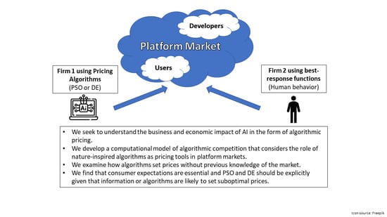
• For pricing, we find that the basic version of PSO works better than the basic version of DE.
• Basic versions of these algorithms are not capable of adapting to changes in consumer expectations.
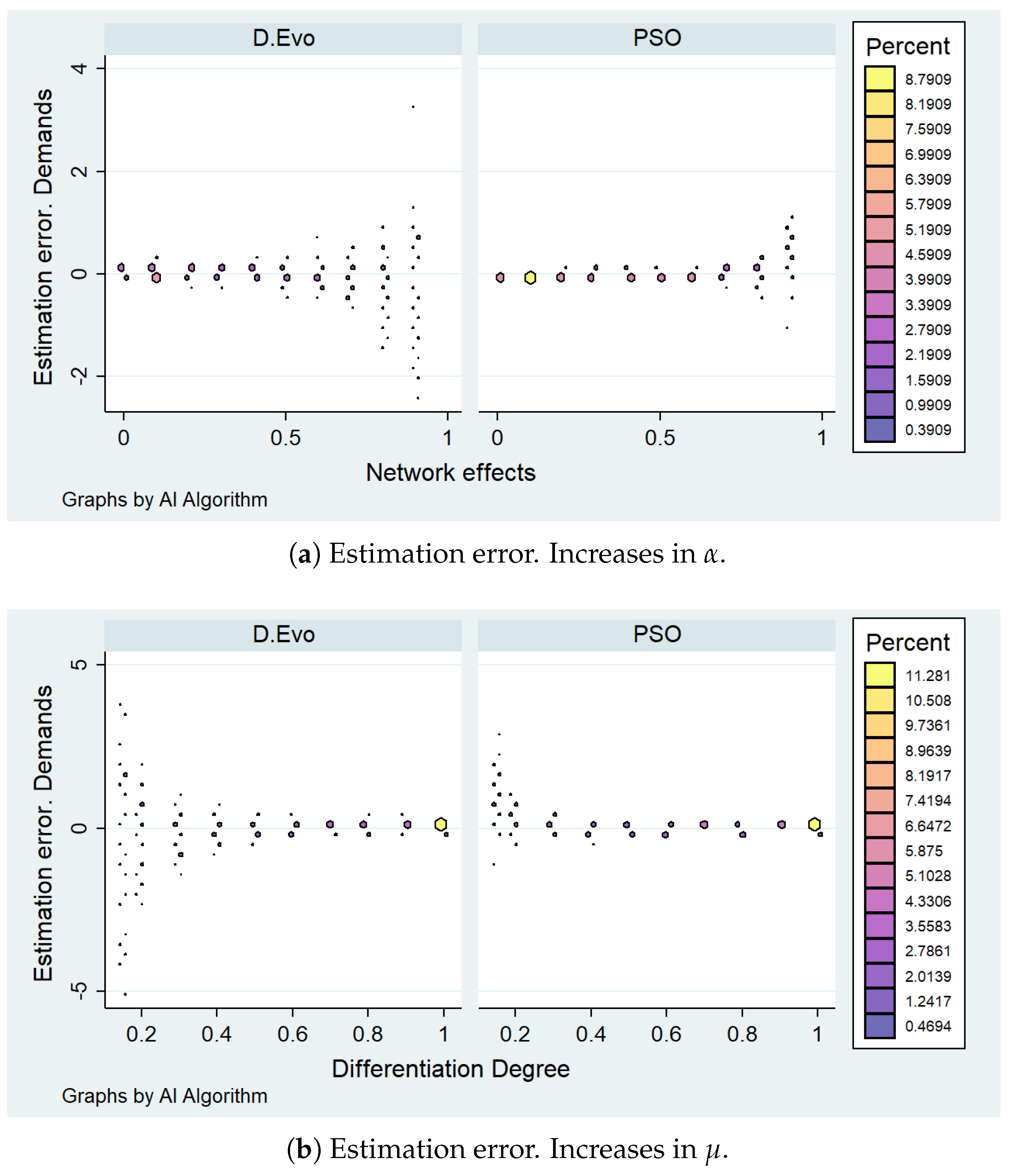
• The more passive consumers are, the more errors both algorithms generate.
• These errors imply that the algorithms set suboptimal prices, which reduces profit.

The rest of the paper is organized as follows. In Section 2.1, we provide a small introduction to biologically inspired algorithms. In Section 2.2, we present the theoretical market that we used to perform our simulations while in Section 3, we present our main results. Finally, we summarize our findings and next steps in Section 4.

2. Materials and Methods

2.1. Biologically Inspired Algorithms

Evolutionary computation is a subfield of AI now used to solve multidimensional problems more efficiently than humans [18]. Although this literature is vast, two algorithms stand out for their simplicity and their links with economic theory: particle swarm optimization (PSO) and differential evolution (DE). Another potential option is genetic algorithms (GAs) but their modeling choices can look arbitrary from an economic point of view (and have a considerable impact on the results), and PSO and DE are more efficient and accurate than many GAs [10,19].

2.1.1. Particle Swarm Optimization (PSO)

PSO is a stochastic optimization technique that generates random points in a multidimensional space (particles) that move towards an optimal solution by sharing information about which points perform better. The idea of PSO came from watching the way flocks of birds, fish, or other animals adapt to avoid predators and to find food by sharing information [20]. This concept is closely related to a trial-and-error process. In other words, we can assume that a company (PSO) tests a limited set of prices (particles) and chooses those prices that perform better (higher profits) and omits those that perform worse. Companies can set the best price given specific market/regulatory conditions by repeating this operation multiple times. Initially, each company considers a set of k potential prices, where k is the number of particles. The position of each particle in the set of real numbers represents a price. Thus, companies can evaluate the performance of each particle (price) in terms of profits. The initial prices are randomly drawn from a uniform distribution between 0 and 1, U(0,1), but as time passes, prices change as new information about their performance is available.

In other words, change in prices (position of each particle) depends on the other prices that generate more profits (locations of the best particles), and such an influence is called “evolutionary velocity ($v_{i,k}$)”. Thus, a price (a particle position) is determined by the best position it has found before ($p_i^l$) and the best price found so far (position of any other particle in its swarm or in the global swarm if there is only one swarm), $p^g$. Formally, the price $p_{i,t}$ at a time t is updated as follows:

$$p_{i,t}=p_{i,t-1}+v_{i,t-1}$$

(1)

$$v_{i,t-1}=w{v}_{i,t-2}+l_1{u}_1(p_i^l-p_{i,t-1})+l_2{u}_2(p^g-p_{i,t-1})$$

(2)

where w is an inertia weight factor representing how past actions (prices) influence the current action (price); $l_1$ and $l_2$ are learning parameters and are called self-confidence and swarm confidence factors, respectively; and $u_1$ and $u_2$ are random numbers uniformly distributed between 0 and 1, U(0,1). In economic games, the payoff of a company also depends on the prices of other companies. Thus, a price that was optimal in a previous iteration may not perform well in the current iteration and vice versa. Thus, $p_i^l$ and $p^g$ may change over time. In fact, at each iteration, we may have new different values for these parameters.

Finally, the inertia weight w in Equation (2) is critical for the PSO’s convergence behavior [21]. There is a trade-off between exploration and exploitation. Thus, we choose a model of exploration that vastly explores at the beginning and, as time goes by, it starts exploiting the best outcomes. Formally, $w_t={(1-w_o)}^t$ where $w_0$ is a constant initial decrease parameter.

2.1.2. Differential Evolution (DE)

Intuitively, differential evolution (DE) also resembles a trial-and-error process. However, the way it is calculated is different. DE is a stochastic optimization technique based on maintaining a population of candidate solutions and creating new ones by combining existing ones according to simple formulas [22]. DE can also be easily interpreted in terms of price optimization. DE resembles a manager who keeps a set of potential prices and makes convex combinations to find the best price before going to market. For example, a company might consider USD 1, USD 5, or USD 10 as prices for its product. This algorithm will make convex combinations of those prices and try to find the best one in terms of profits.

DE has evolved significantly in the last decade, and many variations can be found in the literature. However, we are interested in the simplest version, which is defined by three parameters: the population size ($NP$), the crossover probability ($CR$), and the differential weight (F). Another reason for choosing the simpler version is that our problem is also simple. In fact, our pricing problem is one-dimensional, and the interpretation of the parameters is straightforward. $NP$ represents the set of potential prices that companies may consider. $CR$ represents the incentive to recombine or try new prices. In contrast with PSO, we keep this parameter constant. We make this assumption to show that convergence does not depend on some notion of inertia. In this way, we deviate from the exploration–exploitation trade-off to focus on the action–response process that is closer to the trial-and-error argument or best-response behavior. Finally, F controls the recombination process that generates new candidate solutions. This is the least intuitive in economic terms, but its role will become clear in a moment.

Initially, each company generates a set of NP potential prices. In the first iteration, an item of $NP$ is randomly chosen as the initial price $p_0$. In addition, a new price ($p_m$) is created as a recombination of three random prices (a, b, c) from $NP$. Formally, $p_m=a+F(b-c)$. Companies evaluate the performance of their initial prices in terms of profits and decide whether to test the recombination of prices with probability $CR$. Formally, at time t, companies make the following decision:

$$\begin{array}{cc}CR\ge r\sim U[0,1]& p_{t+1}=\left\{\begin{array}{cc}{p}_t,& \mathrm{If}\pi (p_t,·)\ge \pi (p_m,·)\\ p_m,& \mathrm{If}{\pi }_{(}{p}_m,·)>\pi (p_t,·)\end{array}\right\}\\ CR<r\sim U[0,1]& p_{t+1}=p_t\end{array}$$

(3)

where $\pi (p,·)$ are the profits that depend on their own prices $\left(p\right)$ and competitors’ $(·)$. Therefore, with probability $CR$, companies compare $p_t$ and $p_m$, and with probability $1-CR$, they keep their current prices, $p_t$. This process is repeated over time, testing whether the current or new prices generate more profit. If the new price generates more profit, they stick to that price. If not, they keep the one chosen in the previous iteration. As time passes, other prices may become optimal as new mutations or recombination are tested (either by the company or its competitors). The key challenge facing both algorithms is that the optimal direction or recombinations may become suboptimal. Thus, a priori, it is not clear whether they will be able to reach an optimum if the objective function changes at each iteration as a consequence of the competitors’ behavior.

2.2. Market Environment and Parametrization

We adopted the model proposed by [23] to test our hypotheses. We chose this model because it was analytically tractable and allowed us to address how rational agents behaved under different information scenarios. Other authors adopted theoretical frameworks such as logit, linear, Cournot, or Hotelling models [3,4,10]. However, none of these models consider expectations. In this regard, among the models that allowed us to address consumer expectations, the one chosen was the simplest.

In the following, we present the basic concepts of this model and its main predictions. Figure 1 represents the model. Each company (platform) sets a price (blue arrows) for each consumer group (users and developers). Regardless of the pricing rules, both companies (platforms) try to attract both groups by setting prices that maximize their profits. The main challenge in this model is that platforms have to attract both sides in tandem, and each side forms expectations about what the other side will do (black arrows). In other words, the two platforms compete for two sets of agents (users and developers) that need each other in some way.

Each group (users and developers) has N agents uniformly distributed on a line with unit length, and the two platforms are at locations 0 and 1 on the unit line. The agents’ position on that line represents their tastes; thus, the distance from their position to the platforms represents the disutility of adopting a platform that does not perfectly match their tastes. The model assumes that each agent (user or developer) participates only in one platform, and each agent compares the two platforms and chooses the one that provides a higher utility. To make such a decision, agents consider the price of joining the platform, the intrinsic value of the platform, its disutility with respect to their tastes, and the number of agents from the other group present on each platform. For example, users prefer to join platforms with many developers because that guarantees content (applications, video games, etc.), while developers prefer to join platforms with many users because that guarantees a market for their products. Formally, the utility of users and developers located at $x_j^u$ and $x_j^d$, respectively, from participating on platform i is

$$\begin{array}{cc}{u}_j^u=z-p^i-\mu |x_j^u-l^i|+{\alpha }_u{n}_d^{e,i}& u_j^d=z-v^i-\mu |x_j^d-l^i|+{\alpha }_d{n}_u^{e,i}\end{array}$$

(4)

where $\mu$ captures the level of horizontal differentiation between the platforms and measures the intensity of competition. A smaller value of $\mu$ implies a lower level of differentiation and a higher competition intensity. The mismatch cost, $\mu |x-l^i|$, captures such consumer heterogeneity. Some agents are closer to one of the platforms and find it less costly to consume those platforms. The parameter z captures the intrinsic value of the platform that we assume is high enough to guarantee that all consumers participate. We also assume $\frac{3}{2}\mu <z$, which guarantees that all consumers buy at least from one company. $p^i$ and $v^i$ represent the price paid by users and developers, respectively, for joining the platform i. Finally, each user (and developer) forms expectations about how many developers (users) will join each platform. In other words, users expect $n_d^e$ developers to join, and developers expect $n_u^e$ users to join.

Moreover, we assume the surplus derived by a user from the participation of an additional developer on the platform is ${\alpha }_u>0$, while the profit made by a developer from the participation of an additional user is ${\alpha }_d>0$. Therefore, ${\alpha }^j{n}_{-j}^i$, where $j\in [u,d]$, captures the network effect (i.e., how valuable the presence of the opposite group on the platform is), where $n_{-j}^{e,i}$ is the expected number of agents on the other side of the platform-i. Intuitively, the more people use the services, the more valuable they are.

Following [24], users demands are:

$$n_1^u=\frac{1}{2}+\frac{{\alpha }_u\left(n_d^{e,1}-n_d^{e,2}\right)+p^{\left(2\right)}-p^{\left(1\right)}}{2\mu }$$

(5)

where $j\in [u,d]$. However, how people expect others to join the platform depends on their expectations. In the original model, all developers are informed of all prices and hold responsive expectations about user participation. In other words, their expectations about user participation always match the realized participation, which means that developers are able to forecast how a change in their fees affects users’ decisions and how those decisions affect them, and so on. On the other hand, users can either hold responsive, passive, or wary expectations.

When users are passive, they do not observe the fees paid by developers and do not adjust their expectations if their fees go up or down. If users are wary, they cannot revise their expectations regarding developer participation based on changes in developer fees (which they do not observe). However, users may adjust expectations based on changes in user prices (which they do observe). In other words, when a user sees a change in user prices, they infer that developer-side fees should have changed as well, unlike passive users, who assume that developer prices would not have changed after a change in user prices.

Table 1. Different types of information levels or ways to form expectations. Source: Own.

Information Levels	Intuition
Responsive	Users and developers are aware of the prices paid by all groups
Passive	Users and developers are not aware of the prices paid by the other group (expectations are fixed)
Semipassive	Users are not aware of the developer price, but developers know all prices (expectations are fixed for users but responsive for developers)
Wary	Users do not observe developer prices but infer their price from user prices (expectations are responsive for all agents, but for users, they are more rigid)

shows a summary of these cases and a combination of two that is common in the literature.

Finally, the profits are ${\pi }_i=\left(p_i-c\right)n_i^u+\left(v_i-c\right)n_i^d$, where c is the marginal cost. In all our simulations, profits were the objective function to maximize. Note that profits depended on the company’s own and competitor actions but also on feedback loops from other actions on the other side of the market. Market equilibria were different depending on the assumptions made regarding expectations.

When both platforms recognize that users and developers behave differently, they adapt their pricing. In

Table 2. Price equilibria for each information level. Source: Ref. [23].

Equilibria by Expectations	Developer Price	User Price
Responsive	$v=\mu +c-{\alpha }_u$	$p=\mu +c-{\alpha }_f$
Wary	$v=\mu +c$	$p=\mu +c-{\alpha }_f-\frac{{\alpha }_f{\alpha }_u}{3\mu }$
Semipassive	$v=\mu +c$	$p=\mu +c-{\alpha }_f$
Passive	$v=\mu +c$	$p=\mu +c$

, we show how different expectations affect the theoretical equilibria. However, it is not clear whether algorithms can recognize this without specific instructions. For example, in some cases, algorithms can recognize how users react to prices and adapt their pricing, but it requires simulating a trial-and-error process [25]. It is less clear whether more generic algorithms, such as PSO or DE, can “learn” about these features.

In our experiments, one platform set prices following a classical trial-and-error process that we knew converged to the theoretical equilibrium. On the other hand, the competitor platform set prices using a PSO or DE algorithm, as defined in the previous section. By simulating these interactions between known algorithms in a controlled environment, we could infer whether PSO or DE could deal with different levels of information.

Parametrization

The baseline PSO algorithm consisted of 5 particles $(k=5)$ with $l_1=l_2=1.75$ and $w_0=0.025$. We chose these parameter values to allow cross-comparisons with other works that used PSO for pricing, see [16] or [3]. We also limited the range of evolutionary velocity, $v_i\in [-0.3,0.3]$. This is a common assumption to avoid jumping between corner solutions. Similarly, typical settings in the basic version of the DE algorithm are $F\ge 0.6$ and $CR\ge 0.6$ or $F\in [0.5,1]$ and $CR\in [0.3,0.9]$, see [26,27]. Throughout this paper, we present results when $F=0.8$ and $CR=0.9$.

Although these parameters were fixed during the simulations, we experimented with different configurations. We performed a sensitivity analysis for each algorithm in which we considered ten 5% change steps on the parameters presented in this section, and no significant differences were found. Moreover, we focused on this parameterization because it was common to other works and allowed cross-comparisons.

3. Results

3.1. Baseline Model Responsive Expectations

Only two parameters characterized the theoretical market model, differentiation ($\mu$) and network effects ($\alpha$). Therefore, we considered all combinations of these two parameters to study how the algorithms behaved. Our base case corresponded to the theoretical model in which all agents had responsive expectations. This case corresponded to the same experiments performed by [28], but instead of having two competing algorithms, we had one algorithm and a best-response agent. This case was an useful benchmark to evaluate whether the algorithms were able to learn how to set optimal prices when the competitor followed different behavioral rules.

We know from the literature that algorithms learn to play some notion of equilibria (in some markets) that may be different from that considered by a best-response agent [29]. A key difference in our case is the presence of network effects, which creates the need to address how expectations are formed [30]. Since we were interested in the simplest version of the algorithms, our algorithms were not modified to account for different expectations. Therefore, the main question was whether they could address such differences without explicitly programming them to do so.

In Figure 2, we observe how the algorithms deviated from the theoretical equilibrium when considering the demand. Values around zero meant that the algorithms set the optimal theoretical price. Any deviation from zero implied that the algorithms made errors in setting the optimal price. The theoretical prices we used for comparison were those in Table 2. In this case, we assumed that all players held responsive expectations. Therefore, pricing was symmetric on both sides. The size of each point on the graph represented how common that specific result was. In general, algorithms made small errors, and only when network effects were high or differentiation was low did we observe significant deviations from equilibrium. However, in those cases, the model had two equilibria (one interior and another corner solution) and what we observed was a coordination problem.

When considering prices (Figure 3), we observed a similar pattern, except in the case of the DE algorithm, whose dispersion was large. This happened because the algorithm could not reach the equilibrium but oscillated around it. On the contrary, PSO could set prices closer to equilibrium and showed small deviations as a consequence of its stochastic nature. Putting both dimensions (price and demand) together, it seemed that algorithms could be a tool for pricing in dynamic markets. We found only a few cases in which intervention would be necessary, but these were extreme cases (low differentiation or high network effects). These results provide a rationale for the increasing use of algorithms as pricing tools in digital markets. Note that we used generic algorithms and not tailored versions that might facilitate the way the algorithms set prices. Therefore, it is likely that other versions may improve the performance we observed here.

Finally, we can compare the algorithms head-to-head with the best-response agent. In Figure 4, we show the difference between the profits of the best-response agent and each algorithm. As expected, the gains were equal to or less than those of the best-response agent. However, those cases in which profits were lower were concentrated in the same problematic regions that we discussed before (low differentiation and network effects). Therefore, our first key result should reassure those using PSO or DE-based algorithms as pricing tools, as we found that they worked reasonably well.

3.2. Cases with Different Information Levels

So far, we have assumed that both parties (users and developers) share the same expectations (responsive expectations). However, in some cases, it is more realistic to assume that developers know their fees and user prices, while users only know their prices but have different levels of information about developer fees. In the following cases, we consider three different levels of information, see Table 1. The theoretical equilibria of those cases were characterized by Ref. [23] (see Table 2), but whether algorithms can recognize this situation and set prices accordingly is unclear.

Since the levels of information (or expectations) are independent of the differentiation effect, we did not consider them in the following analysis (the intuitions were the same as in the previous section). However, since expectations are closely related to network effects (or how people expect others to join the platform), we only paid attention to this case. Since we considered different expectation formation processes for users, we focused on how algorithms set prices on this side. Developers behaved as in the previous section, that is, algorithms set prices as before and made minimal errors.

Figure 5 shows the divergence between what the algorithms simulated and the theoretical equilibrium demand in each case. Interestingly, when users were passive, the algorithms could not simulate demands correctly as network effects increased. This happened for both algorithms. Therefore, it was not a problem of a specific configuration or method but of how these algorithms interpreted the network effects. In fact, when we approached the previous case by increasing the “reactiveness” of network effects (semipassive or wary expectations), we observed results closer to the equilibrium (albeit with dispersion). The passive case was an extreme case. It assumed that network effects were present, but people did not react immediately. Our results showed that PSO and DE might have trouble dealing with this case in its basic version if they were not given such information explicitly.

If we look at how these algorithms simulate prices, we have a clear idea of the root of this problem. As shown in Figure 6, when users were passive and network effects increased, algorithms were confused between two equilibria: the real equilibrium with passive expectations (which corresponds to those results around zero) and the equilibrium with responsive expectations (which corresponds to those results with negative difference, lower prices). In other words, in cases where users were passive and network effects were high, the algorithms could increase competition beyond the optimum.

In addition, it could make prices lower than when the best-response agent set prices (e.g., humans). However, this case was not unique. As we observe in Figure 6, when users had semipassive or wary expectations, the algorithms were confused too, but the degree of divergence was not as striking as when users were passive. This result suggested that if algorithms could not account for how users formed expectations or if they assumed generic ways of dealing with expectations, we would likely obtain mixed results when implementing them in real cases.

These results should call for caution when implementing pricing algorithms, as it is likely that the same architecture is used in different markets that share the same set of characteristics, such as differentiation or network effects. Thus, it is critical to address that each market may have different network effects and how they are generated, as our results illustrate. Two markets may highly value the presence of other users, but one may be quite reactive to changes in the user base while the other may be more “passive”. Without taking these characteristics into account, the same algorithm can give good results in our market and suboptimal results in other markets.

Finally, we can look at the profits when addressing the consequences of how the algorithms learn about expectations. More specifically, we can focus on the difference between the profits of a best-response agent and those of the algorithms. In Figure 7, we show that as we increased the network effects, the gap between what a best-response agent and the algorithms earned became larger. This reinforced the previous insights by showing that algorithms might require refinements depending on how people form expectations and should discourage the use of generic solutions.

Recently, we have seen a steady increase in services offering pricing algorithms to retailers. In many cases, this could be an optimal solution for those who cannot track market changes or know little about how to react to competitors. However, it may come at a cost if algorithms cannot adapt (or are not instructed to do so) when network effects are present and expectations differ.

In this regard, note that our algorithms did not address the different ways in which people formed expectations, but only recognized their presence. Intuitively, if algorithms learn from their environment, we can instruct them to recognize the presence of network effects and let them learn from their environment how they are formed. However, we show that this may not be a good idea because when we introduce network effects in their objective functions, we are making assumptions about how expectations are formed. This is the root of the problem that led to the results we presented in this paper. Therefore, we encourage the need to create specific modules for this type of market that are sensitive to the presence of other people.

4. Discussion

Users prefer to join platforms with content or services, and developers prefer to join platforms with a large user base. In other words, digital platforms are based on network effects. The more users, the more developers the platform can attract, and vice versa. In this regard, the economic literature has emphasized that understanding how people form expectations about how others will behave is fundamental to price setting [23]. On the other hand, in recent years, we have observed how simple algorithms without prior knowledge of the market have been able to learn the market dynamics and set optimal prices or even learn to collude [4,5]. These two facts lead to an immediate question: Can simple algorithms learn about how people form their expectations?

In this work, we contributed to the literature by addressing how two well-known algorithms (PSO and DE) behaved when setting prices. The key difference with other works was that we assumed a market with indirect network externalities (users cared about the number of developers, and developers cared about the number of users) in which competitors were best-response agents. First, we showed that when algorithms formed correct expectations, it did not matter if we had algorithms or best-response agents in the market. The market reached its theoretical equilibrium. However, the accuracy could vary depending on the chosen algorithm and the market characteristics. We noted an exception when several equilibria were possible, in which the algorithms exhibited a coordination problem.

Once we had considered that algorithms could not form correct expectations, this problem was exacerbated, and algorithms did not coordinate in theoretical equilibria, leading to a suboptimal solution where competition was stronger than expected. Since algorithms impose a higher degree of competition than usual, this should not worry consumers or the authorities. However, it poses a challenge for companies, as it highlights that algorithms are as dependent as best-response agents on what assumptions we make about the expectation formation process. In this paper, we assumed that the algorithms reacted to network effects. If prices for developers changed, algorithms considered that it would affect users. While that may be true, it imposes a subtle behavior on the algorithms that can lead to suboptimal results, as we observed here.

In this paper, we adopted a basic version of PSO and DE. At this point, some readers may wonder what the impact would be of adopting deep learning methods. On the one hand, they are likely to improve the performance we document here. On the other hand, the literature linking algorithms and their use as a pricing mechanism in economic theory is still in its infancy. In other words, we are still learning the pros and cons of using basic algorithms for pricing. A key challenge is to link specific parameterizations with economic intuitions, which is not always easy or feasible. This is the main limitation so far and poses an interesting problem for future work.

In addition, our results showed that it was necessary to find a way to provide algorithms with knowledge about how expectations were formed. General solutions may not work and may be counterproductive, as our results illustrated. Therefore, even if an algorithm promises faster repricing or more elaborate pricing strategies, a nuanced approach is required. In future work, our goal will be to address how we can help algorithms recognize how consumers form expectations without the need to impose assumptions about network effects.

References

1. Waltman, L.; Kaymak, U. Q-learning agents in a Cournot oligopoly model. J. Econ. Dyn. Control 2008, 32, 3275–3293. [Google Scholar] [CrossRef]
2. Eschenbaum, N.; Mellgren, F.; Zahn, P. Robust algorithmic collusion. arXiv 2022, arXiv:2201.00345. [Google Scholar]
3. Sanchez-Cartas, J.M.; Katsamakas, E. Artificial Intelligence, algorithmic competition and market structures. IEEE Access 2022, 10, 10575–10584. [Google Scholar] [CrossRef]
4. Calvano, E.; Calzolari, G.; Denicolo, V.; Pastorello, S. Artificial intelligence, algorithmic pricing, and collusion. Am. Econ. Rev. 2020, 110, 3267–3297. [Google Scholar] [CrossRef]
5. Klein, T. Autonomous algorithmic collusion: Q-learning under sequential pricing. RAND J. Econ. 2021, 52, 538–558. [Google Scholar] [CrossRef]
6. Sanchez-Cartas, J.M.; Katsamakas, E. Effects of Algorithmic Pricing on Platform Competition; Working Paper; SSRN, 2022; p. 4027365. Available online: https://ssrn.com/abstract=4027365 (accessed on 5 November 2022).
7. Lu, Y.; Wright, J. Tacit collusion with price-matching punishments. Int. J. Ind. Organ. 2010, 28, 298–306. [Google Scholar] [CrossRef]
8. Zhang, Z.J. Price-matching policy and the principle of minimum differentiation. J. Ind. Econ. 1995, 43, 287–299. [Google Scholar] [CrossRef]
9. Werner, T. Algorithmic and Human Collusion; Working Paper; SSRN, 2021; p. 3960738. Available online: https://ssrn.com/abstract=3960738 (accessed on 5 November 2022).
10. Zhang, T.; Brorsen, B.W. Particle swarm optimization algorithm for agent-based artificial markets. Comput. Econ. 2009, 34, 399. [Google Scholar] [CrossRef]
11. Collins, A.; Thomas, L. Comparing reinforcement learning approaches for solving game theoretic models: A dynamic airline pricing game example. J. Oper. Res. Soc. 2012, 63, 1165–1173. [Google Scholar] [CrossRef]
12. Seele, P.; Dierksmeier, C.; Hofstetter, R.; Schultz, M.D. Mapping the ethicality of algorithmic pricing: A review of dynamic and personalized pricing. J. Bus. Ethics 2021, 170, 697–719. [Google Scholar] [CrossRef] [Green Version]
13. Schwalbe, U. Algorithms, machine learning, and collusion. J. Compet. Law Econ. 2018, 14, 568–607. [Google Scholar] [CrossRef]
14. Enke, D.; Mehdiyev, N. Stock market prediction using a combination of stepwise regression analysis, differential evolution-based fuzzy clustering, and a fuzzy inference neural network. Intell. Autom. Soft Comput. 2013, 19, 636–648. [Google Scholar] [CrossRef]
15. Hachicha, N.; Jarboui, B.; Siarry, P. A fuzzy logic control using a differential evolution algorithm aimed at modelling the financial market dynamics. Inf. Sci. 2011, 181, 79–91. [Google Scholar] [CrossRef]
16. Maschek, M.K. Particle Swarm Optimization in Agent-Based Economic Simulations of the Cournot Market Model. Intell. Syst. Account. Financ. Manag. 2015, 22, 133–152. [Google Scholar] [CrossRef]
17. Das, S.; Suganthan, P.N. Differential evolution: A survey of the state-of-the-art. IEEE Trans. Evol. Comput. 2010, 15, 4–31. [Google Scholar] [CrossRef]
18. Bonate, P.L.; Howard, D.R. Evolutionary Optimization Algorithms: Biologically Inspired and Population-Based Approaches to Computer Intelligence; John Wiley & Sons: Hoboken, NJ, USA, 2013; ISBN 978-0470937419. [Google Scholar]
19. Lampinen, J.; Storn, R. Differential evolution. In New Optimization Techniques in Engineering; Springer: Berlin/Heidelberg, Germany, 2004; pp. 123–166. [Google Scholar]
20. Eberhart, R.; Kennedy, J. Particle swarm optimization. In Proceedings of the IEEE International Conference on Neural Networks, Perth, Australia, 27 November–1 December 1995; Volume 4, pp. 1942–1948. [Google Scholar]
21. Chatterjee, A.; Siarry, P. Nonlinear inertia weight variation for dynamic adaptation in particle swarm optimization. Comput. Oper. Res. 2006, 33, 859–871. [Google Scholar] [CrossRef]
22. Storn, R.; Price, K. Differential evolution–a simple and efficient heuristic for global optimization over continuous spaces. J. Glob. Optim. 1997, 11, 341–359. [Google Scholar] [CrossRef]
23. Hagiu, A.; Hałaburda, H. Information and two-sided platform profits. Int. J. Ind. Organ. 2014, 34, 25–35. [Google Scholar] [CrossRef] [Green Version]
24. Armstrong, M. Competition in two-sided markets. RAND J. Econ. 2006, 37, 668–691. [Google Scholar] [CrossRef] [Green Version]
25. Sanchez-Cartas, J.M. Agent-based models and industrial organization theory. A price-competition algorithm for agent-based models based on Game Theory. Complex Adapt. Syst. Model. 2018, 6, 1–30. [Google Scholar] [CrossRef] [Green Version]
26. Zielinski, K.; Weitkemper, P.; Laur, R.; Kammeyer, K.D. Parameter study for differential evolution using a power allocation problem including interference cancellation. In Proceedings of the 2006 IEEE International Conference on Evolutionary Computation, Vancouver, BC, Canada, 16–21 July 2006; pp. 1857–1864. [Google Scholar]
27. Storn, R. On the usage of differential evolution for function optimization. In Proceedings of the North American Fuzzy Information Processing, Berkeley, CA, USA, 19–22 June 1996; pp. 519–523. [Google Scholar]
28. Sanchez-Cartas, J.M.; Sancristobal, I.P. Nature-inspired algorithms and individual decision-making. In Proceedings of the 5th International Conference on Decision Economics, DECON, L’Aquila, Italy, 13–15 July 2022; In Press. [Google Scholar]
29. Asker, J.; Fershtman, C.; Pakes, A. Artificial Intelligence and Pricing: The Impact of Algorithm Design; Technical Report; National Bureau of Economic Research: Cambridge, MA, USA, 2021. [Google Scholar]
30. Evans, D.S. Some empirical aspects of multi-sided platform industries. Rev. Netw. Econ. 2003, 2, 191–209. [Google Scholar] [CrossRef]
Figure 1. Algorithms, platforms, and relationships in this model. Source: Own and Freepik.com.
Electronics 11 03927 g001
Figure 2. Demand estimation by parameter. Left = network effects; Right = differentiation. Source: Own.
Electronics 11 03927 g002
Figure 3. Price estimation by parameter. Left = network effects; Right = differentiation. Source: Own.
Electronics 11 03927 g003
Figure 4. Difference between algorithms and a best-response platform. Left = network effects; Right = differentiation. Source: Own.
Electronics 11 03927 g004
Figure 5. Demand estimation error. Source: Own.
Electronics 11 03927 g005
Figure 6. Price estimation error. Source: Own.
Electronics 11 03927 g006
Figure 7. Difference in profits between the best-response agent and algorithms. Source: Own.
Electronics 11 03927 g007