1. Introduction
The United Nations has proposed 17 actions known as Sustainable Development Goals (SDGs) for reducing poverty, protecting the planet and ensuring peace and prosperity for the entire world by 2030. Number six of these goals is “Ensure availability and sustainable management of water and sanitation for all”. Some of the actions for achieving this include improving water quality by reducing pollution, increasing water use efficiency and managing water resources. Therefore, better monitoring of water and sanitation interventions is essential for achieving this SDG in a more cost-effective and efficient way.
The use of the Internet of Things (IoT) in the monitoring of water consumption and quality is a very active field of research [
1,
2]. However, a key issue for universalizing proposals, as SDGs fulfilment needs, is the relatively expensive cost of equipment, mainly intended for large water-management companies. The challenge is to achieve efficient water-monitoring systems at an affordable cost. For this reason, various initiatives are currently aimed at the design and commercialization of low-cost equipment for monitoring water consumption and quality, for instance, water-quality monitoring equipment for use in the context of Citizen Science [
3] or water-meter designs to be deployed in hand pumps of Africa [
4,
5].
In fact, water monitoring is not a single point problem as it typically requires several sensor nodes that can communicate amongst themselves. In this regard, several communication technologies have been analyzed to determine if they are suitable for application in these environments [
6]. In the specific case of wells and water sources located outside urban and suburban areas, long-distance communication infrastructures are required, with SigFox and LoRa being fairly good options. The difference between them is mainly that LoRa is based on a Do-It-Yourself (DIY) approach that does not require the infrastructure provided by a telecommunications operator and therefore does not depend on its coverage.
In addition to data communication, there is a complementary aspect related to data collection. In many cases, a large amount of information is collected for use in subsequent processing calculations, analysis and decision making [
1]. The bandwidths available for the sensor node data can be too low to allow pass-through of all data, in both the LoRa and SigFox technologies [
6]. To alleviate this problem, the amount of monitoring data to be transmitted is typically reduced in two ways: (1) by reducing the sample rate and (2) by preprocessing the information in the nodes.
Reducing computational time, energy or resources because at a certain moment an “exact” prediction of a model is not necessary, is not a novel idea. In fact, it is an emerging computing paradigm known as approximate computing [
7]. Examples of this are the use of floating point formats with less precision [
8], which have been shown to be effective in achieving energy efficiency at the cost of obtaining a result that is accurate enough for the purpose of the calculation, but no more. Influence of arithmetic precision, data uncertainty and modelling uncertainty on prediction capabilities depend strongly on specific characteristics of the problem in hands.
In this work, we propose a low-cost device with LoRa communication technology that monitors the water flow and electrical consumption during pumping from deep boreholes/wells, and that predicts the water level evolution using a simplified model of the aquifer. The proposal follows not only an approximate computing but an edge-computing approach. This later paradigm focuses on the preprocesses and computation of outputs of interest directly at the nodes, minimizing the needs of bandwidth and of time delay to inform of the predictions at the node. Recording data from water meters and energy sensors is straightforward, but real-time computation and estimation of water level evolution is not. Both, the approximate and edge computing perspectives are used in the proposal to minimize use of energy and communication resources.
Estimating the water level of a water well is neither easy nor cheap. Normally these types of systems have a price that can be too high if a number of wells need to be monitored. The advantage of our approach is that it does not require an expensive infrastructure to collect these data since the necessary measurement equipment is affordable, automatable and would be present in the same device. The proposed system has been introduced, validated and analyzed in a deep well pumping for irrigation in the middle part of the Matarraña river basin, a tributary of the Ebro river, Spain. The area is characterized by a arid-mediaterranea climate, with annual precipitation about 600 mm. The big aquifer “Puertos de Beceite” (number ES091MSBT096 in the Ebro river basin characterization and planing [
9]), is below the upper part of the basin. In the middle part, still in a mountain context, there are smaller aquifers in conglomerates and Oligocene sandstones, typically confined at high depth, and of relatively reduced productivity. The uncertainties associated to aquifer modelling are high, and the impact of pumping in the water table is sometimes significant, which makes it an illustrative example for the proposal.
The main contributions of this work are the following:
a low-cost device with a “do-it-yourself” metering and communication approach for analysing water production and energy consumption of pumpings, specifically designed for deep boreholes/wells;
the computation of an approximated model in the device for predicting water-level change due to pumping;
a complete description of all hardware and software aspects of the proposed device;
a comprehensive analysis of the feasibility of the proposed device in terms of temperature, power consumption and performance;
the practical application of the presented device in a real environment.
The paper is organized as follows:
Section 2 presents the state of the art of water monitoring systems and their data acquisition, transmission and processing approaches.
Section 3 identifies the existing problems in the current measurement systems as well as the requirements of the proposed solution.
Section 4 presents an overview of our proposal.
Section 5 and
Section 6 provide the hardware and software details of the proposal, respectively. The validation of the device in terms of temperature, energy consumption and performance is shown in
Section 7.
Section 8 describes the deployment of the proposed device in the real application. Finally,
Section 9 summarizes the main conclusions.
2. Related Work
Water monitoring systems help to identify the state, changes and trends of water resources, infrastructures and services. Data acquisition, transmission and processing are three of the main stages that can be identified in these systems from a data-analysis perspective.
2.1. Data Acquisition
Water monitoring systems usually acquire data with local devices located in the same place of action. These devices generally incorporate several specific sensors to analyze the chemical, physical or biological properties. For instance, they can measure the oxygen level to determine the health of the ecosystem, pH level to measure the acid or base quality of the water, electrical conductivity to assess the purity of the water, degree of salinity to estimate the concentration of dissolved salts in water, turbidity to analyze the relative clarity of a liquid, or temperature to detect thermal pollution, among other properties. Beyond the use of local sensors, remote sensors can also be used for data acquisition. In this way, Andres et al. [
10] also provide a description of various techniques for monitoring water and sanitation by collecting data with satellites or even unmanned aerial vehicles. In general, images collected by cameras and other spectral instruments are used in a wide range of wavelengths.
In our proposal, data acquisition is limited to electrical power consumption [
11,
12,
13,
14] by submerged pumping, and water flow [
15,
16,
17] throughout a water-meter.
2.2. Data Transmission
Data transmission can deal with several types of wireless (radio, satellite, cellular, WiFi, Bluetooth, etc) and wired (DSL, coaxial cable, fiber, etc) communication technologies. It is a key challenge in water monitoring systems, particularly in environments where there is no power outlet and the system’s operability depends on the battery life. Although nowadays batteries have a greater longevity, their charge is still limited to a certain amount.
Wireless Sensor Networks (WSNs) are a reliable and efficient approach for achieving a scalable and secure network to deliver data by means of interconnected sensor nodes that monitor physical or environmental conditions of a given place of action. Therefore, they have been widely used in fields as diverse as environmental protection, intelligent transportation of goods, human health, disaster prevention, military intelligence, and many more. Water monitoring also uses this type of network. Zhang et al. [
18] present a water-monitoring system based on wireless sensor networks to be used in breeding aquatic plant and animal species. The proposed wireless sensor network ensures that the monitored data are received in real time and are reliable, and also makes the sensor devices operate for a longer period of time. Adu-Mani et al. [
19] provide an overview of several quality-monitoring systems, mainly focusing on data transmission by means of wireless sensor networks. They highlight the low level of security that this type of network incorporates and the difficulty in keeping them operational for long periods of time because there is no continuous power source. Finally, Calderwood et al. [
20] developed an automatic network of low-cost, open-source wireless sensors for real-time monitoring of groundwater using acoustic sensors. This fully functional and operational proposal is compared to equivalent commercial systems that are several times less expensive in monetary terms, mainly due to the processing and visualization environment built with free software.
In summary, WSNs are a group of sensor nodes connected without a cable to collect some data, but there is no direct connection to the internet. In contrast, any IoT system should always have present the internet and involves anything that can be connected to it. In this way, IoT has recently gained attention as a potential approach for water monitoring as it allows information to be exchanged among various devices and data collected in real time to be analyzed to take appropriate corrective measures. Geetha and Gouthami [
21] provide state of the art techniques and tools used in existing intelligent water-quality control-systems and also introduces a simple and smart approach based on IoT technology. A real implementation of a groundwater level monitoring network was deployed in Nova Scotia, Canada [
22]. In this case, low-cost Internet-of-Things devices transmit the data collected through custom made meters to visualize and compare the water levels in real time of several domestic wells of private users. In other areas of action, it should be noted that access to healthy and clean water is a key challenge in most communities around the world. Traditional water-dispenser systems usually break down within a few years and they are not often fixed since there is no maintenance revenue. eWaterPay [
23] is a solution that uses mobile technology, IOT and Near-Field Communication (NFC) technology to solve this problem. Ingram and Menom [
4] analyze the robustness of this system in terms of accuracy of the flow meter and flow rate.
The Low Powered Wide Area Network (LPWAN) is a wireless system that enables long distance data transmission and devices to be connected with a low energy consumption approach. They appear as a valid transport protocol option for certain needs of the IoT. Examples of LPWAN technologies are LoRa, Sigfox and Weightless. In particular, the LoRaWAN [
24,
25,
26,
27,
28,
29] protocol has been widely proved to be an effective way of transmitting and receiving quick data with battery-operated devices in scenarios with low power requirements. For instance, Pietrosemoli et al. [
30] outline the design of a simple and affordable device to obtain weather data from commercial weather stations with a limited wireless range and retransmit the data to cover long distances by means of the LoRaWAN protocol. Cano-Ortega and Sanchez-Sutil [
31] use LoRaWAN to build a prototype that monitors induction motors of electrical machines. This proposal benefits from secure communications, low energy-consumption and a long signal-range both outdoors and indoors. On the other hand, Dayana et al. [
32] integrate a LoRaWAN module into an electric meter to send details of the users’ electricity consumption. They achieve a wide range of information transmission, lower energy use and non-significant data loss. You et al. [
33] propose applying the enhanced LoRaWAN security protocol in the context of efficient parking management in smart cities. They achieve a significant improvement and better performance in terms of network latencies compared to previously applied approaches. Finally, Nakamura et al. [
34] propose a flexible architecture for situations with limited resources located in remote rural areas. The main idea of this proposal is that it adopts LoRa technology to allow long-range transmissions with low-power consumption from sensor nodes to a central node, that transfers the data to the server via the internet.
Focusing on water monitoring, LoRaWAN is becoming a popular technology for data transmission due to its substantial advantages in terms of performance, energy consumption and cost. Ngom et al. [
35] apply LoRa technology in a water-quality monitoring system of a pool in a botanical garden, in which data were previously collected by manual measurement. They show that this protocol together with a low-cost infrastructure for capturing and processing data in real time can achieve an efficient and reliable water-monitoring system. Miles et al. [
36] carry out a LoRaWAN study to determine whether it is the most suitable communication network to be applied in smart agriculture. The authors experimentally model an open farm concluding that LoRaWAN has a lot of potential for IoT applications. Apart from these more experimental and personalized proposals, there are already commercial water sensors and water-monitoring systems (for instance Telog-41 of TrimbleWater [
37] and DO-IoT-Compact of Umweltleistungen [
38]) on the market that use low-power LoRa technology so that the sensor batteries last for several years with fairly reasonable data transmission intervals. Finally, there is a very interesting project at La Marina de Valencia (Spain) proposed by Battulga et al. [
39]. In their project they use a network of sensors deployed throughout the sea to measure parameters such as the weather and the movement of marine vehicles. This sensor network uses open-source software and LoRaWAN communication technology to transmit the collected data to a fog computing platform that processes the data in real time. This project is similar to the one proposed in this work, except that in our case the real-time data processing to make decisions is carried out in the sensor node and not only from real data but also from estimated data.
2.3. Data Processing
Data processing for identifying the pumping influence in the aquifers has been widely researched in the past, directly linked to the development of physically based theories and mathematical models representing aquifer behaviour [
40,
41,
42,
43,
44]. The first models dealt with confined aquifers, in simplified geometries, and typically in contexts of constant flow pumping and posterior recovery. At times they have been the only option for estimating aquifer hydraulic properties. Nowadays, it is a topic that still arouses interest due to the difficulty in estimating aquifer characteristics; and as a first step to solve the partial differential equations representing realistically 2D and 3D heterogeneous aquifers and systems of aquifers.
Non-constant water flow can be modelled by superposition principle, provided that the math model is kept linear. Mishra et al. [
45] introduce an analytical method for confined, unconfined, and leaky aquifers that focuses on numerically transforming discrete pumping rate data signals into the Laplace transform domain (as proposed by Roumboutsos and Stewart [
43]) but avoids numerical instabilities by means of a discrete-time convolution integral. A special case of non-constant water-flow is found when the pumping is performed at constant-head pumping. Trabucchi et al. [
46] extend Agarwal’s method [
42], which is based on recovery tests combined with mathematical models for water-level estimation.
Recall that historical data of instantaneous water-flow rate and instantaneous pumping electrical real power-consumption are needed in order to compute estimations for the water level using simplified analytical solutions and qualify the fulfilment of underlying hypothesis (constant flow rate, or constant head pressure). Thus, their availability is mandatory for the data processing of the water table evolution.
3. Problem Statement and Requirements
The main aim of this work is to monitor the extraction of water from a well and to predict the evolution of the position of the water table within. Thus, not only to have an estimation of the instant position of the water table, but also to provide expected future evolution of it. In order to predict these values, a simplified modelling of the energy balance of the pumping scheme, plus an approximation to the water mass balance in the aquifer are used. Prediction depends on magnitudes characterizing the pumping periods and can be computed at the device. Water table evolution during non-pumping periods, referred usually as recovery, depends on previous pumping periods. It is not the goal of this approach to be used to monitor water level position without pumping, just measuring it.
There are several ways to directly measure the water level, each with its advantages and disadvantages. It is possible to use tape measures, sonic sensors or piezometric sensors [
47]. The tape measure is manual, while the sensors are automatic. It means a relatively cheap initial investment for tap measure, but its cost is high in the long term as well as inefficient, since it requires labor and travel to perform the measurements. Instead, sensors are usually with devices which automatically computes and transmits the water level values but at non-reduced costs. For instance, prices of sonic probes or piezometric probes range between EUR 500 and EUR 1200 [
48]. Piezometric probes require the installation of sensors within the borehole, in contact with water, and they are pre designed to work with certain ranges of pressures, which represents an additional limitation in boreholes with large withdraws. Sonic probes are non invasive and can be used to track deep water level locations, but the accuracy, even high (errors less than 1%), can represent a problem for water levels in tens (or even a hundred) of meters.
For these two main reasons, costs and high-but-insufficient accuracy for real-time control of pumping, we propose an alternative approach based on the approximate and edge-computing paradigms. The proposal requires the measurement and recording of pumped water and electrical power consumption. The position of the water table is directly related to the water pressure within the aquifer, and this is influenced by the real power of the pump, energy losses in the water pipes, the pumping history, but also by the geometric and material characteristics of the aquifer and their water recharge mechanisms. Aquifer data are usually the most uncertain. However, main characteristics of time-dependent solutions can be checked in advance, and model parameters can be calibrated with punctual real-data of water table evolution during a pumping–recovery sequence.
A water-meter with pulse emitter is the simplest way to approximate instantaneous water flow within a pipe. Water-meters are designed to produce a reduced water energy loss at nominal water flow rates; additionally, they are usually installed to have a minimum control of the pumping use (and typically they are required in legalized pumping schemes in most countries). Water meters with pulse emission type MJ-SDC can obtain the information digitally in order to transmit it later. There are devices that measure the amount of water that passes through them at a reasonable price unless the remote transmission of the information is also required. For instance, prices of Zenner, Woltman and AO-Electronics range between EUR 300 and EUR 1200 with remote transmission functionality, and between EUR 50 and EUR 300 without this remote transmission functionality AlphaOmega Electronics [
49], NingBo Water Meters [
50]. In addition, a clock will be necessary that, through a small electronic circuit (microcontroller/PLC), can calculate the water flow rate.
Energy power consumption can be measured with voltmeters and ammeters. Similarly to the water-meters, their cost is quite reasonable unless the functionality of remotely transmitting the collected information is necessary. For instance, prices of voltmeters and ammeters range between EUR 60 and EUR 1200 with the remote transmission functionality, and between EUR 30 and EUR 60 without this remote transmission functionality [
51]. For single-phase current measurements, a voltmeter and an ammeter are sufficient, however, for three-phase current measurements, three voltmeters and four ammeters are recommended to not depend on the hypothesis of balanced system functioning.
Finally, to provide data communication between the extraction points and the centralized server system, we need solutions that do not depend on commercial cellular networks, since distribution companies would not build large communications installations because the territory is rural, remote and there is little possibility of recovering their investment. The most common and low-cost solutions such as Bluetooth and Wi-Fi, are not considered either because they have a very short communication range. Therefore, our solution must cover our communication needs, which are: (a) distances of several kilometers, (b) rural locations with little or no commercial communication infrastructures, and (c) little need for bandwidth (a few bytes per second).
In summary, although there is a large number of commercial solutions, they tend to have a high cost in monetary terms. To the best of our knowledge, there is no device on the market that can measure or estimate the behavior of a well and that can be replicated at a reasonable cost. We proposed a device with a minimum cost of EUR 200 per unit (within EU in 2019) for three-phase pumping.
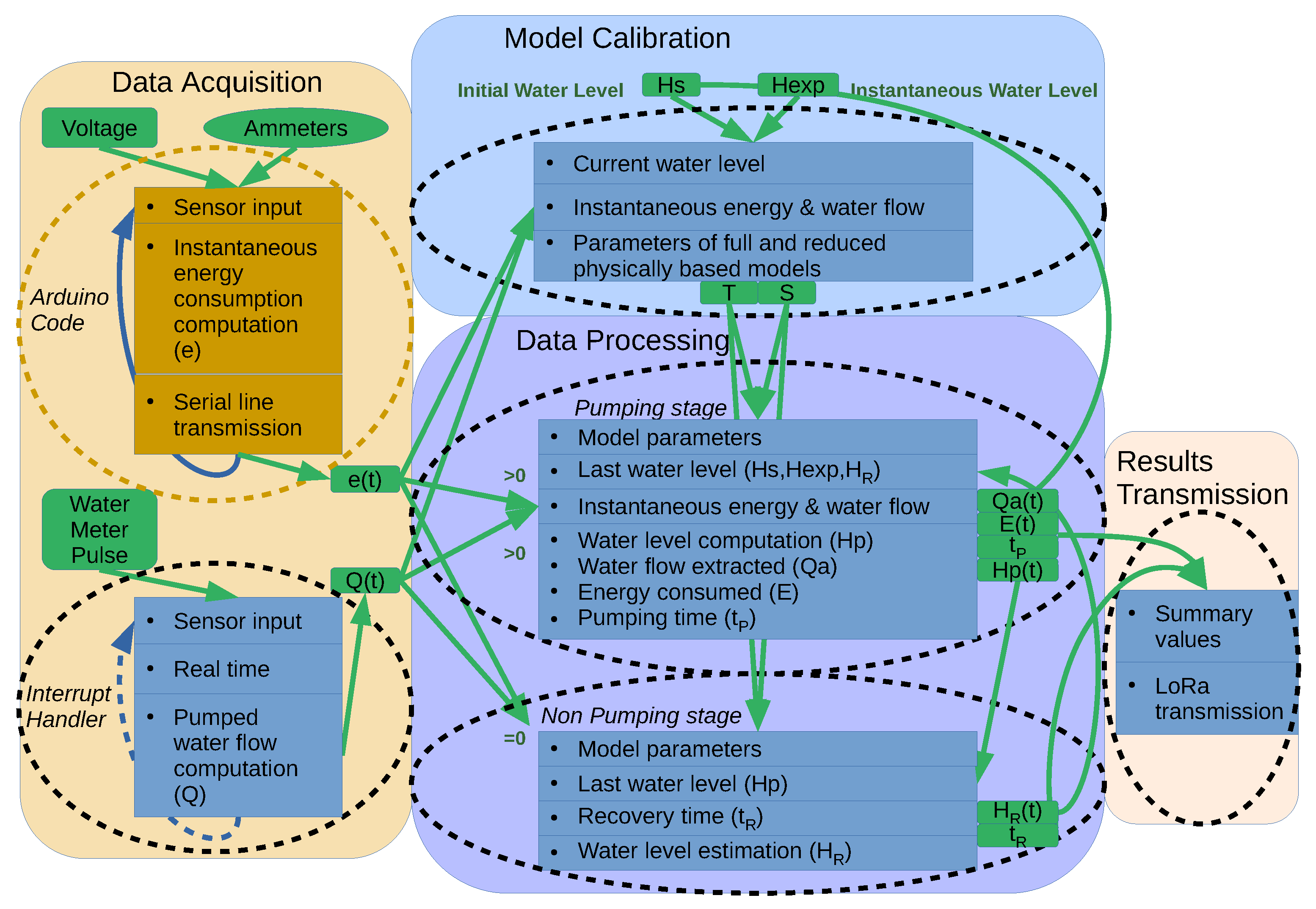
4. Proposal: Overview
Figure 1 shows the data flow scheme that we propose for our monitoring system in which four main stages can be distinguished: (1) Data Acquisition, (2) Model Calibration, (3) Data Processing and (4) Results Transmission. The Data Acquisition stage is responsible for obtaining data from the different sensors (energy consumption and flow meter). The Model Calibration stage includes the calibration of the model parameters, only once, combining data with the data from the acquisition stage with direct water table evolution measurement. The model can be calibrated as many times as necessary, but a priori only once would be sufficient for normal system operation. The Data Processing stage is responsible for estimating the water level and the behavior of the well based on the model calibrated and the new data obtained from the acquisition stage. Finally, the Results Transmission stage sends the data through an appropriate communication system to the server or end user. Notice that the model is calibrated once and the behavior of the well is calculated constantly and in real time.
Voltmeters and ammeters are used to measure power energy consumption. In a three-phase system, electricity intensity by phase and neutral, and the voltages between phase and neutral are of interest. Sensors are connected to a microcontroller that through an Analog-to-Digital converter can obtain instant values of all magnitudes, and compute the RMS value of intensities, voltages and real and apparent powers by line. This can be efficiently computed using a rapid FFT (Fast Fourier Transform) transform of signal data. Note that RMS magnitudes needs a minimum sampling time to be computed which depends on electricity frecuency.
For measuring the water flow, the on–off signal of the pulse emitter is recorded. The instantaneous water flow rate can be approximated considering the constant water volume characteristic of each water-meter and the time increment between signals. The average water flow from pumping start depends on total time and total number of signals emitted.
A water level meter (300 m) has been used for manually measuring the water level. Data collected is used for model calibration and validation off-line. Model parameters are updated in the device for the computations during Data Processing stage.
The microcontroller receives the real-time data from the sensors, computes the estimated water level position, and makes the necessary transmissions through the installed communications system.
There is a wide range of microcontrollers on the market, but in our case we rely on those that are widely recognized and accepted and that have a large range of user-tested hardware and software extensions. In this sense, the de facto standard based on Arduino and Raspberry Pi are the most suitable. Nowadays there is a great interest in the use of Arduino and Raspberry Pi systems, either individually or combined, for low-cost monitoring environments. In this way, we can identify several examples that combine Arduino and Raspberry Pi, such as to control the temperature of a photovoltaic generator [
52] or to manage the charging process of an electric vehicle [
53], and examples that deal with Raspberry Pi individually, such as for photovoltaic water pumping systems [
54] or for monitoring the energy performance of buildings [
55].
Arduino is a Plug and Play microcontroller. As soon as it is plugged in, it starts executing the single program that has been loaded. This is programmed in C/C++ and is developed and compiled in the Arduino IDE environment from a PC, and then transferred to the microcontroller through a USB connection. As it is a single program, it must integrate all the functionalities that our application needs, and therefore it is not very flexible to modifications and extensions of functionalities. However, it is suitable for performing a single repetitive task efficiently and effectively, such as measuring RMS real power consumption. In this sense, any board that has AD converters and the possibility of communication via serial line would be sufficient.
On the other hand, Raspberry Pi, being a whole computer, with a Linux operating system installed and access to all the development software and Linux libraries, offers great flexibility to be programmed in any need and can be easily modified and expanded. It has 40 well-known input/output pins, with a series of integrated adapters (USB, Ethernet, etc.) and a storage system based on MicroSD cards, where the operating system and the applications that we need are located. Among them, any compatible board would give equivalent results (Raspberry Pi, Asus Tinker, Lepotato, Rock64, Banana Pi, Orange Pi, Odroids, PocketBeagle) and within the Raspberry Pi family there are some alternatives available that have sufficient computing power, from the Pi Zero to the Pi4.
As outlined above, we require a communication approach that can cover distances of several kilometers in an environment with little communication infrastructure and low bandwidth needs. These requirements made us consider than the LPWAN (Low Power Wide Area Network) style protocols are suitable. Of these technologies LoRa and LoRaWAN are considered the most appropriate, given that these communication protocols are in full expansion and fit perfectly into the characteristics of the needed communication. In fact, LoRa is a wide spectrum modulation technology with a high network range and low power consumption at the cost of low bandwidth compared to other wireless technologies. However, this is not a problem since our device only generates a small volume of data.
In summary, we will use an Arduino micro controller for real power consumption, and a Raspberry Pi to record real power, water flow, interpolate both temporal series, compute water level and proceed to communicate at desired time-intervals. The included sensors are ammeters, voltmeters and a pulse of the water meter. Finally, the communications system used is the LoRa technology.
5. Proposal: Hardware Aspects
This section describes the selected low-cost solution proposed in this work. It describes the different components necessary to take measurements, perform calculations and transmit the results for the correct modeling of the behavior of the water well.
Figure 2 shows the block diagram and the real image of the hardware prototype. Particularly,
Figure 2a depicts the main components of the single-phase board prototype and the internal and external connections, and
Figure 2b shows an image of the single-phase prototype with its main boards, sensors and interconnections.
5.1. Selected Board: Arduino + Raspberry Pi
For the acquisition of electricity data we chose an open source solution from the company LeChacal. This company offers various kits, which by means of an Arduino controller and a series of voltage and ampere sensors are capable of measuring the electricity consumption that passes through a cable. Specifically we chose the RPIZ_CT3V1 kit [
56], which is the kit that can be integrated easily with a Raspberry Pi Zero [
57], and the RPIZ_CT4V3 kit with Raspberry Pi 3A+ or 3B+ [
58] for the three-phase current system. This already microprogrammed kits acquires the data from its sensors and performs the consumption calculation, giving values of RealPower in watts, Irms in milliamps and Vrms in volts. This information is sent through a serial line and can be collected through the serial port
/dev/ttyAMA0 of a Raspberry Pi, as described in the company’s tutorial. This kit has installed, and uses, the YHDC-SCT013 current sensors [
59] and a AC/AC adaptor-voltage sensor IdealPower 77DE-06-09 [
60].
Raspberry Pi boards offer enough computing power for our needs, are priced very affordably, and integrate seamlessly with the Arduino microcontroller from LeChacal. These systems have been installed with the Raspbian Lite version based on Debian 10.0, which offers all the programs and services of an entire Linux system. We also have all the power of a Linux system to perform extra calculations and communications with the outside world.
The pulse emitter of the water-meter has been connected to three GPIO of the raspberry Pi: one pin to ground, another pin to 3v3 voltage and the third to data on GPIO17. The internal Arduino pull-up resistor is used to protect the circuit and two LEDs with their resistors have been added to visualize the on–off signal of the water meter. Remarkably, some water–meters emit pulses of predefined length once a volume of water has been detected. Others, the most basic models, emit an on–off signal directly from the reed switch on the counting wheel. At constant water flow, time of pulse is less than 0.5 of time of a wheel round. Unequal pulses are better registered as on–off and off–on changes. The water volume per round depends on the meter and the counting wheel with the sensor installed.
A separate battery clock was installed to provide accurate time at all times, corresponding to the RTC PI v3 kit from ABelectronicsUK [
61]. This board makes it possible to keep the real time while the system is off and/or disconnected from a power outlet. Finally, tests were carried out with USB devices for the communications part, specifically, a Fast-Ethernet USB-RJ45 device and a LoRa LilyGO-TTGO-LORA32 device [
62].
5.2. I/O and Communication
Following an ascending order, we discuss the different ways in which the system components communicate. On the one hand, the SCT-013 current sensors and the AC/AC adaptor-voltage sensors are connected via a three-pole jack (although only two are used) in an analog way to the Arduino RPIZ_CT3V1 board. This in turn is connected to the serial port of the 40-pin GPIO bus of the Raspberry Pi Zero W/Pi 3 board. Between the two boards, the RTC PI v3 real time clock is also connected to the 40-pin GPIO bus. Finally, the connection of the water meter is made with a two-pole jack that is connected directly to one of the digital input pins of the GPIO of the Raspberry Pi.
The whole system is powered by a 5V USB power supply. External communication is carried out through the Wi-Fi built into the Raspberry Pi and can also be carried out through the USB connector, where a USB-RJ45 Ethernet device can be plugged in. The communication tests with LoRa were carried out with LilyGO-TTGO-LORA32 devices, which allow easy installation and use in the Raspberry Pi board.
5.3. Board Assembly
It is not difficult to assemble the components and it is possible to Do-it-Yourself. You just have to follow the manufacturer’s assembly instructions for building the different components (they can be accessed from the references). As can be seen in
Figure 2b, the ammeters surround the current cable that they want to measure, in this case and for single-phase current they cover both the phase cable (brown) and the neutral cable (blue). We can also see the cables from the water meter (black and red), which are the ones that connect to a GPIO port of the Raspberry Pi.
6. Proposal: Software Aspects
In this section we present the system’s operating. First, we discuss the general mode of operation, then the different algorithms that are executed, next the water well-modeling software and finally the communication mechanism used.
Figure 3 details the dataflow and code that are executed on the devices. Particularly, the block marked in a dashed orange circle corresponds to the code that is executed on the Arduino board while the blocks marked in dashed black circles correspond to the codes that are executed on the Raspberry Pi.
6.1. Operating Mode
The procedure to take measurements begins as soon as the two devices are plugged in: the Arduino and the Raspberry Pi. From that moment on, the Arduino microcontroller, which already has the program to run, begins taking measurements from the sensors, calculating the current values in real time and sending the values through the serial line to the Raspberry at a preconfigured cadence (values between 1 and 5 s).
The Lite version of Raspbian, that is based on Debian 10.0, has been installed in the Raspberry Pi system and through an installed service it starts a script that executes the water well-modeling program. As values are obtained, the well-modeling algorithm is applied to calculate the water level in real time. Once the water extraction is completed, the summary values of the extraction that has been carried out are sent with the LoRa protocol at a predetermined rate by the program settings. Typically, the devices do not turn off between different water withdrawals but when the exploitation is stopped (seasonally, weekly, power interruption, etc). In order to minimize the risk of file system data corruption and loss of data, the writings to file are always accompanied by the flush command, and thus it is guaranteed that the writing is performed on the physical device.
6.2. Stage Algorithms
As it is shown in
Figure 1, our approach is divided into several stages to estimate the behavior of the well: (1) Data Acquisition, (2) Model Calibration, (3) Data Processing and (4) Results Transmission. Each of these stages has its own code to perform the tasks assigned to them. In the following subsections we describe each of these codes in detail.
6.2.1. Data Acquisition
The data acquisition stage is responsible for obtaining data from the energy consumption sensor and flow meter sensor. These data will be used in the following stages.
The energy consumption acquisition code runs on both controllers in the system (Arduino board and Raspberry Pi board). The RMS values are calculated in the Arduino board by reading the data provided by the voltage and amp sensors. The code that the Arduino board executes is the one provided by the LeChacal company as part of the energy consumption measurement kit. The results are sent through the serial line to the Raspberry Pi board. The Raspberry Pi board executes a code that is constantly reading through its serial line and realizes some preprocess to generate real power data and save them with a time stamp. It is important to note that data are received by passive waiting, and in this case, as long as no new data arrive, no CPU is consumed by the Raspberry Pi processor. The frequency of sending and receiving the values can be configured. A minimum of 0.2 s for sensor reading and RMS computation is needed (10 cycles with electricity at 50 Hz), thus values over 1 s are proposed.
The flow meter acquisition code is in charge of receiving pulses generated by the water meter that is at the outlet of the well pump. This pulse is connected to a GPIO pin in the Raspberry Pi. The GPIO signal handles an interrupt routine, executed each time the signal changes. Because of this passive waiting, CPU utilization is very low. Each time a change is detected, code saves the time of the change and computes instantaneous and mean pumped water-flow since beginning.
6.2.2. Model Calibration
The model calibration stage is responsible for calibrating the model parameters which characterize water level evolution. These parameters are related to different terms appearing when considering water mass balance in the aquifer and energy balance in the pumping system. We choose a reference model based on expected aquifer characteristics: The
Theis model [
40], which corresponds to the analytical solution of the boundary value problem of the water pressure in the aquifer for a simplified case (confined aquifer of infinite extension, homogeneous, horizontal and with a constant thickness, with a small diameter pumping borehole totally penetrating the aquifer strata, and with a constant pumping flow starting instantaneously at time zero). In these conditions, the aquifer response is characterized by two material coefficients: Transmissivity,
T, and storativity,
S. The water pressure draw down is given at a distance
r of the borehole center and at time
t starting at
, by
, with
,
, and
the constant flow rate. In single well contexts
, the radius of the borehole is considered representative of the real water table position, thus the water level evolution is given by
, with
the initial water level position referred usually as static level (level without previous pumping influences). Model unknowns
T and
are unlikely to change once determined, but the static water level can be expected to suffer changes occasionally. Even the reality of the aquifer does not fulfil previous hypothesis for the
Theis model, the two parameters
T and
S are the basis for more complex aquifer modelling.
We calibrate aquifer parameters with the model considering non constant flow pumping and both pumping and recovery periods. Superposition cannot be applied to each variation of the real–time signal, few seconds. We assume near to constant head pumping conditions and adjust an exponential interpolation of for each pumping period, fitted with a penalized minimum least square problem to force the capture of the total water volume. Optimization is solved with a genetic algorithm. Finally, the inverse Laplacian of the analytical solution on the Laplace space is computed. We apply superposition principle for recovery and to include influence of past pumping in subsequent pumping–recovery periods.
As the reference model cannot be solved repeatedly on a real-time basis, we propose using the Jacob’s approximation to
Theis solution, considering the average water flow previously pumped,
, as the reference constant water flow. The classical Jacob’s approximation is found considering only first two terms of the approximation of
by a series, obtaining
, valid for
. In the case of recovery after a pumping period of
time span, the superposition principle leads to
. After rearranging, water level during recovery is found as
, with
related with
T. For pumping periods we use a storability-alike parameter,
, which differs from the one characteristic of the aquifer and calibrated previously with the full model. The use of two storability parameters was previously found useful by [
63], and discussed by [
64]. In our approach, the storability-alike parameter for pumping captures the influence of time lapse between start pumping and the water meter signal and possible changes on water head. Thus, water level during pumping is approximated by
, with
and
related to
T and
. Additional terms can be included in
and
to consider the impact of previous pumping periods in actual simulation. Summarising, model calibration of hydraulics requires the calibration of four parameters, involving both the reference and the simplified hydraulic models, and with data involving pumping and recovery periods (
and measured
).
On the other hand, the power effectively transferred from pumping to water is transformed into energy losses by friction of water flow with pipes and valves system, potential energy, i.e., increment of water height with respect to initial position, and kinetic energy, which is assumed negligible. Water energy losses can be considered proportional to square water flow rate in standard operational conditions (with limited water flow velocity inside the pipe). Energy transferred with pumping is given by the pump curve, which is provided by the manufacturer, and relates the increment of water pressure with the water flow, usually, with a quadratic function and referred to nominal power. Water level can be approximated considering energy balance by , with the real power time evolution and the instantaneous water flow. A minimum of three parameters are needed to relate water level position during pumping with water flow and real power consumption, with two characterizing the pump. These parameters are calibrated using least squares with , and measured data during pumping. Note that during pumping periods, both mass and energy balance should be fulfilled, which implies .
6.2.3. Data Processing
The data processing stage estimates the water level and the behavior of the well based on the model calibrated in the Calibration stage and the new data obtained from the acquisition stage every time an extraction is made.
With no pumping active (, ) water level estimate is the static water level . In case that there has been a previous pumping recorded is computed from and values (the pumping time span and the total water volume pumped). When pumping starts, signal of increases from near zero to nominal pumping power in a period of some, even tens of, seconds. During this time water starts flowing up through the pipe until it reaches the water meter and water provision point. It can delay up to a couple of minutes. Then water meter signal indicates the water flow .
With pumping active ( and ) the proposed prediction for is equal to . The value of is considered an indicator of the error of the estimation . Recall that real time computation is based on an approximated model, which could not be accurate in the short term after starting. Both computations, and , are linear combinations of powers and cross products of , , and . Pumping finishes once real power consumption drops to zero, which implies no pumping and stopping water flow. The water meter last signal is previous to last real power signal clearly above zero.
6.2.4. Results Transmission
The results transmission stage sends the data through an appropriate communication system to the server or end user. In this way, LoRa communication is used to wirelessly connect all the well pumping stations of an aquifer with the server. LoRa is able to communicate small amounts of data over long distances with low power consumption; however, unfortunately, latencies can be very high. This means that LoRa is not suitable for sending real-time data or control commands from the server in the event of an error. The supervision of the operation, as well as the detection and action in the event of an error, is programmed in the microcontroller of the pumping station, following the Edge Computing approach. Therefore, LoRa communication can be used to inform the server of problems or errors in the pumping station; however, it is not feasible to wait for orders or commands from the server.
The data generated by the sensors are also processed locally in the Raspberry Pi microcontroller. As shown in
Section 7.3, CPU usage for this processing is low and can be carried out easily in the microcontroller. Therefore, once they have been processed, the data to be transmitted to the server will be summaries of a water extraction and values of the behavior of the well and the underlying aquifer. The communication period is long, from minutes to hours, and therefore LoRa offers enough bandwidth for our needs. Each LoRa data communication will send just a few values: pumping starting time, duration of pipeline transport, pumping end time, total extracted water and average power consumption. Therefore, the LoRa communication protocol meets our needs for a minimum communication infrastructure, low bandwidth needs and long-distance communication in rural environments (a few kilometers).
Figure 4 shows the throughput experimentally obtained with TTGO LORA32 test devices. Two devices, one as an emitter and one as a receiver, have been used in a laboratory environment separated by a few centimeters from each other. The throughput obtained in a given SF (spread factor) with different message sizes has been measured. Particularly, SFs from 7 to 12 with message sizes ranging from 1 byte to 200 bytes have been tested. Results show that low SFs (SF7 and SF8) have a higher throughput (4900 bps and 2800 bps) compared with throughput (400 bps and 214 bps) obtained with high SFs (SF11 and SF12).
Given these specifications, we will use low profile LoRa settings that make sufficiently effective communication possible. With this idea, for measurements of a small number of water wells, high SFs (spread factors) of 11 or 12 will be used, since they have sufficient bandwidth and allow transmissions at a greater distance (10 to 20 km). The biggest disadvantage of these SF is that they occupy the transmission channel for a longer time. On the other hand, for a basin with a greater number of wells, the communication parameters of each of the wells could be configured differently. Configuring the closest wells with lower SFs of 7 or 8, which occupy less channel time, have greater bandwidth, but have a transmission distance limited to a few km (2 km approximately). As the wells get further away from the server, they would use higher SFs that allow greater transmission distances, and SF 12 would be used in those that are further away.
In summary, LoRa communication fits perfectly in this approach as we deal with low rates of data communication, long range distances, low power requirements, and there is no need to communicate real-time data or commands.
7. Proposal: Verification
This section presents the validation of the device in terms of power consumption, temperature and performance. A prototype that is powered by single-phase alternating current was used in the laboratory. The simulation of the pulses of the water meter was obtained from a pulse generator. The main target of the test is to determine the limits of the device at room temperature and at high temperatures in the shade. In both cases, the CPU usage is varied from idle to 100%, going through the normal usage it would have while taking measurements from the well.
7.1. Energy Consumption
Power consumption is very important in battery operated systems. However, in our case the highest energy consumption is produced by the water-pump motor. It varies a lot depending on water flow and well depth. Values from one thousand to several tens of thousands are typical. The sensors and microcontroller used have very low energy consumption (from 1 W to 4 W), which can be several hundreds of watts less than the consumption of the water-pump motor (from 1000 W to 10,000 W), which means that the consumption of the box represents less than 0.4% of the total energy consumed.
7.2. Temperature
The safe working temperature for a Raspberry Pi, for all its components, is from 0 °C to 70 °C (Celsius degrees) and the working range of the SoC/CPU is from −40 °C to 85 °C [
65]. Two types of temperatures are measured: first the SoC temperature (by reading the internal temperature sensor) and second the temperature inside the box (with a DS18B20 temperature sensor connected through 1-wire to another Raspberry Pi that is outside the box).
A series of experiments were carried out with different external temperatures and different CPU loads on the Raspberry PI to check the temperature limits in execution of the selected boards.
Table 1 shows all the experiments carried out in the laboratory.
Box and SoC temperature measurements were made at an ambient temperature of 20 °C and 40 °C. These measurements, in turn, were carried out under three operating conditions of the Raspberry PI CPU. The first in an Idle state, with no program running, the second with a program running the well-modeling code while it is taking measurements of power consumption using voltmeters and ammeters, and measurements of an electronic pulse that indicates turns of a flowmeter (it was simulated with a pulse generator every 2 s), and the third executing a code (stress) that uses the CPU at 100%.
Figure 5 shows the evolution of the temperature of the two sensors that were used in the two ambient temperature experiments (20 °C and 40 °C), while the use of the CPU is modified, from idle, through execution of the modeling code, until using the CPU at 100%. It is worth mentioning that the use of the CPU is altered by the experiment itself, since the measurements of temperature and the use of the CPU of the SoC are made with the Raspberry PI itself; therefore, initially the CPU already starts from a CPU usage of 5%. This is not a problem for our experiment, since we are looking for the upper limits of the running temperature of the system. Just say that these initial values will have a slightly lower temperature. However, the temperature of the box has been taken from another external Raspberry PI and in this case it does not alter the CPU usage of the internal Raspberry PI.
As shown in
Table 1, in any of the six situations, the limit temperature of the Raspberry and Arduino boards is not reached. We highlight the case of executing the modeling code at an ambient temperature of 40 °C where the CPU temperatures are between 50 °C and 54 °C and the box is between 43 °C and 46 °C.
7.3. Performance
In this section, we evaluate the cost in CPU consumption of different alternatives for model calibration and data processing codes. Reference and simplified models are calibrated with codes developed in the R language (R is a free software environment for statistical computing and graphics [
66]). Libraries GA v 3.2.2 [
67,
68] and Pracma v. 2.3.8 [
69] are used. Data acquisition and processing stages at the Raspberry Pi are performed in codes written in Fortran 90. Data acquisition stage at the Arduino is written in C. For comparative purposes, Cython and Python versions of the Fortran code for data processing has been developed. Cython [
70] is an optimizing static compiler for Python, so we can obtain additional performance by executing compiled code instead of interpreted Python code.
Table 2 contains the execution time of the five codes considered: R-dp (for data process stage), R-cal-GA (for calibration stage), and F90-dp (in Fortran 90), Cython-dp and Python-dp corresponding data-process codes. These codes were executed in four systems with diverse computing powers: a Xeon+Quadro workstation (server), a Laptop computer with Celeron CPU, and two models of Raspberry PI (PI 4 and Pi Zero W). Only the Raspberry PIs are suitable for our purposes, but the more powerful laptop and server systems give us an estimation of the minimum execution times for these codes.
It can be observed in
Table 2 that the R-cal-GA is the code that takes the longest to execute, followed by the R-dp, and the Python, Cython and finally Fortran 90 versions. Cython is about 10% faster than Python, and Fortran twice faster than Cython. Regarding the four computing systems tested, the fastest is the server, followed by the laptop, then Raspberry Pi 4, and Raspberry Pi Zero W (the slowest one). Although it is the slowest system, the Raspberry Pi Zero W is fast enough for data acquisition and process stages. Raspberry Pi 4 is an option for R-calibration-GA code, but twice time slower than the laptop.
Table 2 also shows %CPU usage data for the five codes and four computing systems, as the average value for a period of 1 h of execution. As mentioned above, despite being the slowest system, Fortran and Cython codes executed in Raspberry Pi Zero W last between 2 and 4 s (in 1 h), that is, less than 0.1% of CPU usage. It is not necessary to have a more powerful system.
Finally, in
Figure 6, we analyzed the effect of the number of input data samples in the execution time of the five versions of the code in the four considered computing systems.
Figure 6a–d correspond to the execution times (in seconds), while
Figure 6e–h show the relative time of the Python code version (
) compared to the other code versions (
) and computed as
. In general, the execution time increases with the volume of data to process, except the R-cal-GA code, with an almost constant execution time (because the data processing represent a small percentage of the total execution time, compared with optimization computations). From the slowest code to the fastest one, we have R-cal-GA, R, Cython, Python and Fortran 90 “dp” versions, as seen in
Table 2. Regarding the four computing systems, the server is one order of magnitude faster than the Laptop, the Laptop computer is slightly faster than Raspberry Pi 4, and our Raspberry Pi Zero W is about one order of magnitude slower than Raspberry Pi 4, but powerful enough to execute the data capture and process stages, with the lowest energy consumption.
8. Field Case Application
To test and validate the proposal, a prototype was installed in an operational pumping for irrigation in the Matarraña valley. The tested prototype is for a three-phase current supply. The case study is characterized by a reference static water level m and a radius of the perforation of m. The aquifer is confined and the pump is located at 130 m. Pump curve is given by m/w, m s/(w dm) at nominal real power of w.
Two sets of data including manual measurement of water level evolution are available: First, 11 January 2019, and second, 11 April 2019. The first involves one pumping–recovery period and it was used to calibrate the model. The second set includes three consecutive pumping–recovery periods, although third is covered partially. Information from April is used to validate the model. They were not performed in same conditions, a situation that is detected by the error indicator during validation. In the following, main results for calibration and validation are commented. The first pumping period is used here for the recalibration of the model, and two strategies are compared: automatically, in the sensor, and off-line.
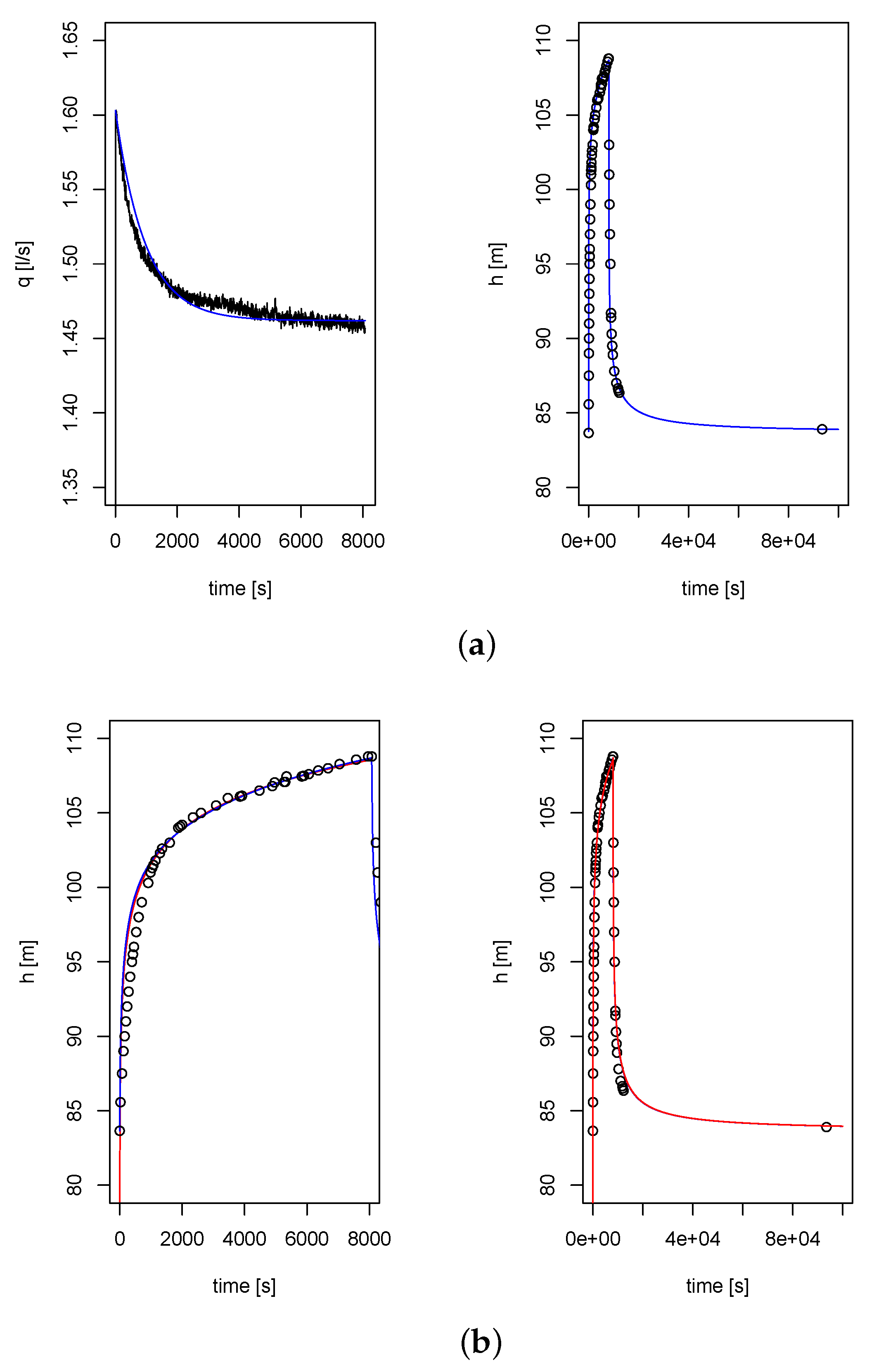
The water flow and real power consumption during calibration case are shown in
Figure 7. The pumping duration was approximately 2 h and 15 min, and it was performed with almost constant head conditions. Note the delay in the starting time of water flow (at surface) with respect to real power starting curve, about 50 s. Water flow starts at 1.6 L per second and finishes at 1.4, a reduction of 15%.
Two sets of parameters provide good results with the full model: one for better adjusting the pumping and the other for recovery. Other pairs in between provide also acceptable results. Even the values are quite different. Differences are in the usual range and they are in agreement with
T values reported in the area (from 0.28 to 158 m
/day [
9]). Values of parameters and corresponding constants are indicated in
Table 3.
Figure 8 summarizes main results of calibration for both sets of aquifer parameters. First, left to right, the water flow adjusted by an exponential function from experimental data is shown. Total water volume is represented with an error less than 0.05%. Second, the water level evolution simulated with the reference model and first set of parameters is depicted. Results are graphically in very good agreement. Third and fourth are the results with the second set of parameters, during just the pumping period or including recovery, with both reference and simplified models. The results of both models are almost indistinguishable. The error during the recovery of second set of parameters is slightly higher than first set, and it can be identified in
Figure 8; but adjustment for pumping is slightly better.
The parameter related to water energy losses due to pipe transport is calibrated using the real power data, obtaining
m s
/(dm
). With all parameters adjusted, results of the simulations with both sets of parameters are presented in
Figure 9. The estimated water levels
are indicated in red color, overimpressed to the orange curves corresponding to
. Measured data are plotted in black. Both results are in good agreement with data. The error diminishes with time, being less than 1% of
H except during the first 10 to 15 min. Overestimation of first set of parameters is larger the second one during this starting time.
Figure 10 shows the results obtained when applying calibrated set of parameters to the data of first pumping of the validation case. Remarkably the results given by the aquifer model are in very good agreement with experimental data; but energy does not provide correct estimators (orange curve) and therefore model estimate (red curve) is incorrect. This fact is detected by the error indicator which does not converge to zero with time. This is in agreement with the documented change in water provision.
Figure 10 shows the evolution of the error in terms of water flow rate. Most of the time the error is around 6.5 m. A simple estimate of the water energy losses parameter is given by the mean value of the error, discarding staring time. This gives
m s
/dm
for 1st set of parameters and
for the second. Note that these values can be updated during the data process stage with a simple computation (arithmetic mean). The value can be also updated with least squares considering the water level measured data, off-line, in the calibration stage. This later result is similar to previous ones
m s
/dm
, and common to both cases as it is computed directly from measured water level data.
The parameter
which characterizes simplified hydraulic modelling has been recalibrated with first pumping period of validation. Results are indicated as
in
Table 3. Variations with respect to calibration are low, specially considering the overall range of variation of this parameter. Results are indistinguishable with the second set of parameters. There is a slightly larger difference (not reproduced here) with the first one.
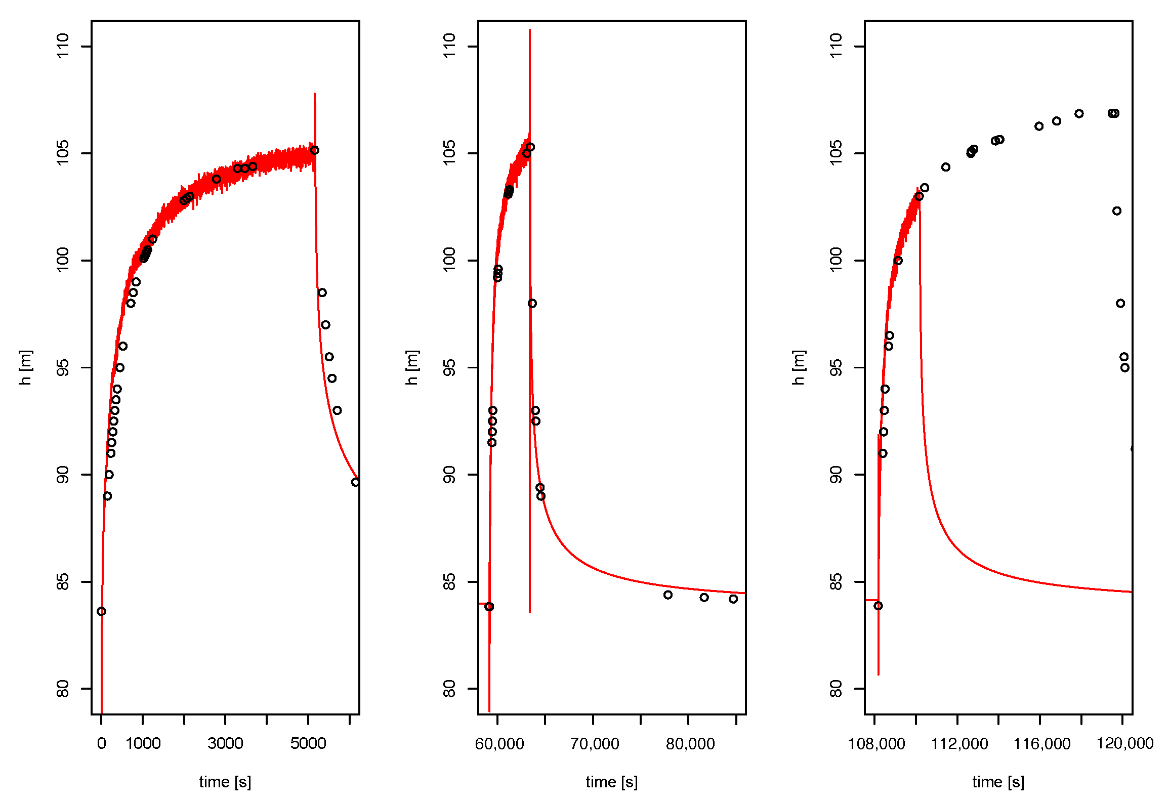
Figure 11 shows the estimated results for the overall validation period. Errors during staring pumping and recovery are significant, punctually of 5% of
H with the second set of parameters. However, most of the time are close to zero. The signal during the third pumping period was lost, thus the model predicts the recovery water table evolution from this time forward. Without real-time information of real power and water flow rate the model fails to predict water table evolution. Three details of the overall validation test are presented in
Figure 12. The results are in very good agreement, except during transitions between recovery–pumping, for a short period of time.
9. Conclusions and Future Work
Water is currently a scarce and precious good and, therefore, mechanisms for managing it that are affordable, particularly for those communities with limited resources, should be provided. In this work we introduce a low-cost water monitoring device a LoRa communication approach. The device performs measures of real power consumption, instant and accumulated water flow, an estimates the present and future location of the water table in a fairly precise way. The proposal only needs off-line computation for calibration of system parameters in terms of measured water level evolution during a pumping–recovery cycle, which makes it possible to reduce communication costs.
This device has been tested and evaluated in a laboratory environment in terms of energy consumption, temperature and performance. The energy consumption of the device is negligible compared to that of the monitored water pump. The device always operates in safe temperature ranges even in the worst conditions. The execution of data process stage with Fortran or even Python is fast enough in the cheapest hardware system (Raspberry Pi Zero W) with a CPU usage as low as 0.1%. Moreover, the proposed device was also tested in a real environment and its deployment shows that it is being very effective in evaluating the location of the water table.
Our proposal introduces some limitations due to the different decisions that have been taken in its design. First, a number of simplifications of the well/aquifer behavior implicit in the Theis and Jacob model have been assumed and calibrated, but the actual well/aquifer behavior might differ slightly over time, thus some kind of periodic calibration processes would be necessary. Secondly, our device incorporates two microcontroller boards, but another approach could have been the use of a single microcontroller board providing a cheaper and more compact solution. On the other hand, the number of input/output ports dedicated to data sensors is determined by the current selection of Raspberry Pi and Arduino boards and, although it is suitable for our approach, it would not be very scalable assuming monitoring or control of complex irrigation systems. Finally, as our proposal is a do-it-yourself device, it can be difficult to use it in massive environments and also in technologically isolated areas, due to the need for end-user training for correct maintenance, or specialized technical services in the implementation areas.
As future work, it is intended to efficiently deploy several prototypes of the device presented to build a distributed system along pumping systems sharing the same aquifer, so the different nodes can share the measurements and take into account crossing influences in the water level evolution of ecah one. Model extensions to deal with more complex aquifer modelling are expected to accurately reproduce other cases.


