A Refined Taylor-Fourier Transform with Applications to Wideband Oscillation Monitoring

Abstract

The recent increase in renewable energy adoption has enhanced the penetration rate of electronic equipment, leading to an increased risk of wideband oscillations. Existing wide-area measurement systems mainly focus on fundamental phasors, which cannot effectively monitor wideband oscillations. This study presents an accurate wideband oscillation monitoring method based on radial basis function (RBF) neural networks and Taylor–Fourier transform (TFT). First, discrete Fourier transform is used to obtain a preliminary estimation of the oscillation signal, and then, TFT is adopted to obtain a precise estimation even under dynamic conditions. To reduce the computational burden of TFT, an RBF neural network is used for noise intensity estimation, which adaptively determines the window length. Finally, the proposed method is verified by synthetic data and the field data collected from Guyuan and Hami, China. The experimental results show that the RBF neural network has an excellent denoising effect. When the signal-to-noise ratio is 45 dB, the maximum overall phasor error and the maximum frequency error are 1% and 0.01 Hz, respectively. Hence, it is expected to be useful for next-generation monitoring systems.

1. Introduction

In recent years, numerous renewable energy sources, such as wind and solar, have been connected to the power grid by using power electronic equipment [1,2,3], gradually forming a ‘double-high’ power system characterised by a high proportion of renewable energy and a high proportion of power electronic equipment [4,5]. However, weak disturbance rejection, low inertia, and strong coupling caused by power electronic equipment have severely affected the safe and stable operation of power systems [6], which can easily cause wideband oscillation accidents. For example, the doubly fed induction generators in Texas, USA, caused sub-synchronous oscillation (SSO) accidents for oscillation frequencies of 20–30 Hz [7,8]; a sub-and super-synchronous oscillation accident occurred in Hami, China [9]; an oscillation accident at the frequency of 1.4 kHz occurred in the France–Spain networking project. Such incidents may lead to equipment damage, tripping of renewable energy units, and a wide region of power failures. According to the proposal of China’s ‘dual carbon’ target, renewable energy penetration will further increase in the near future and the ability of the grid to withstand wideband oscillations will be further challenged [10].

Model-based methods, such as time-domain simulation and state-space modelling, have been widely used for wideband oscillation analysis [11]. However, these methods have a common challenge: accurate system models at wideband frequencies are not easily accessible. Consequently, measurement-based monitoring and analysis have garnered considerable attention. Corsi et al., reported that for uncertain system models, constructing a wide-area monitoring system for wideband oscillations is an effective means of analysing oscillation characteristics [12]. Analyses can be conducted based on monitoring data, including oscillation risk assessment, root-cause analysis, and countermeasure design Refs. [13,14,15]. Moreover, constructing a wideband oscillation monitoring system is the hardware foundation for real-time early warning, control, and protection.

Wide-area measurement systems based on phasor measurement units (PMUs) have been used in power systems worldwide. However, the PMU only focuses on the fundamental phasor [16,17], which makes it challenging to meet the demands of wideband oscillation monitoring. To address this issue, researchers must update the PMU algorithm to make it applicable to wideband measurements. At present, the common methods of wideband oscillation monitoring include the Fourier transform, wavelet transform, Hilbert–Huang transform (HHT), Kalman filter, and Prony. In [18,19], the windowed interpolated discrete Fourier transform (IpDFT) was combined with filters for oscillation parameter estimation, which is accurate for stationary signals. However, this method fails when the oscillation signals are non-stationary. In [20,21], wavelet transform was applied to process time-variant signals; however, this resulted in low resolution when multifrequency components were processed. In [22,23], the HHT algorithm was employed to identify oscillation parameters, but the endpoint effect and mode-mixing related to HHT were not addressed. In [24,25], a Kalman-filter-based algorithm was used to track wideband harmonics; however, the algorithm requires many predefined parameters and is computationally expensive. In [26,27], a morphological filter was combined with the wavelet transform and Prony algorithm to improve the anti-noise performance. In [28], intrinsic time-scale decomposition (ITD) was utilised for monitoring the subsynchronous oscillation, which is simple and feasible for real-time monitoring. However, a relatively stationary signal was considered for all the aforementioned algorithms. The stationarity assumptions lead to large errors for wideband oscillations with strong time-variant characteristics.

The Taylor–Fourier transform (TFT) method performs better because of its dynamic phasor model; therefore, it is efficient in wideband oscillation monitoring [29]. However, the TFT algorithm requires a long window length [30] or an elegant filtering preprocess [31] because it is very sensitive to noise. As indicated in extensive tests, mitigating the influence of noise on TFT by using conventional filtering methods is challenging unless a very high-order filter is used. However, the high-order filter significantly increases the calculation time, and the delay degrades the real-time performance of the TFT method. Therefore, increasing the window length is still the most effective way to enhance the performance of TFT under noisy conditions.

This paper presents an adaptive-window-length-based TFT for wideband oscillation monitoring. The idea is to adaptively determine the TFT window length based on the estimated noise level. As a result, the computational and dynamic performance of wideband oscillation monitoring can be optimised. The main contributions of the paper are summarized as follows.

(1)

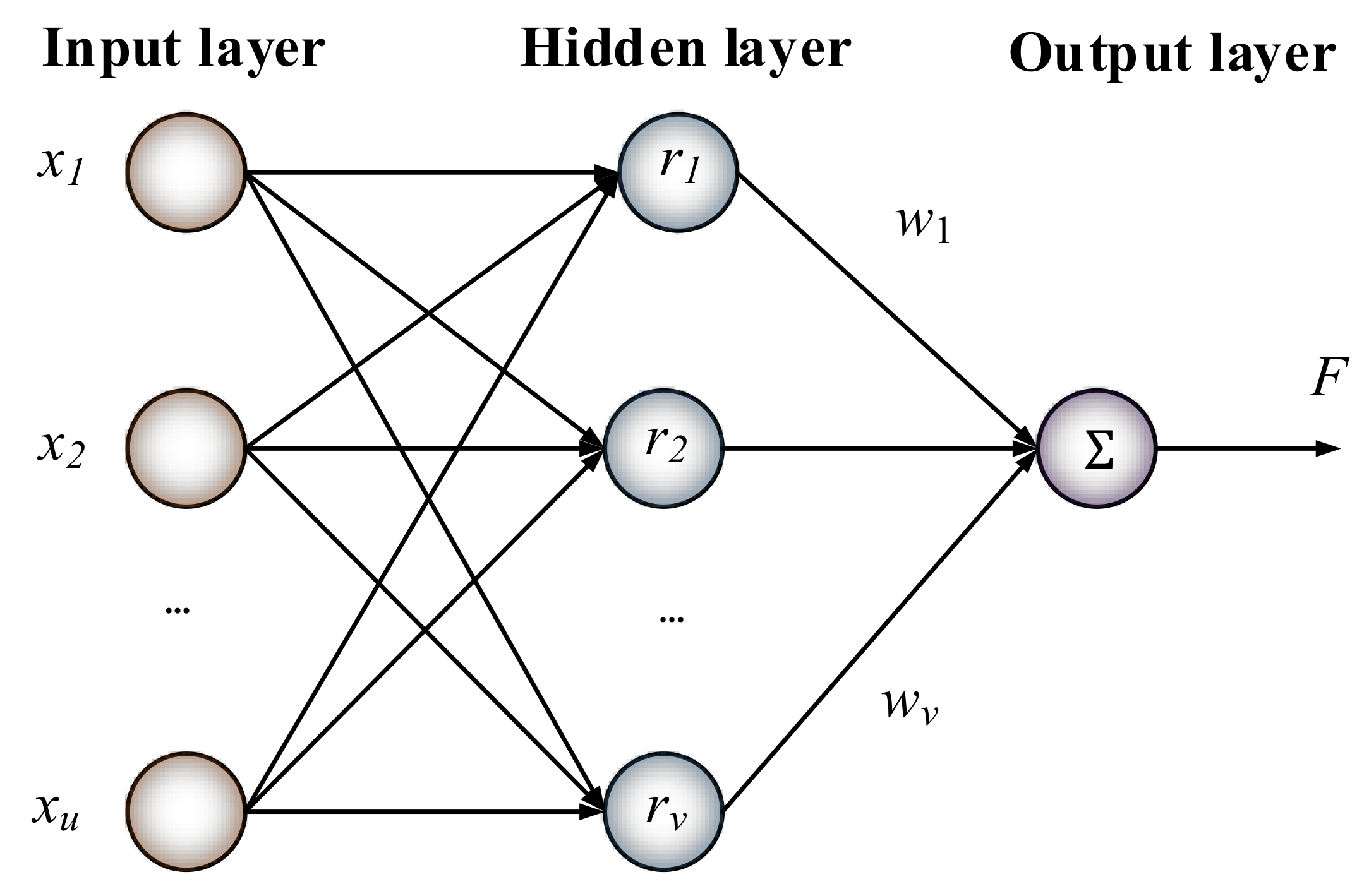
A radial basis function (RBF) neural network is adopted to estimate the noise level, which can approximate any nonlinear function with arbitrary precision and has the advantages of global approximation capacity, compact topology, and fast convergence.

(2)

An adaptive window length is designed based on the noise level. The window length is designed to be longer when the SNR is low, which strikes a good balance between dynamic performance and estimation accuracy.

(3)

Numerous simulation tests are conducted with field data from Guyuan and Hami incidents. The results indicate that the proposed method is feasible and robust for practical applications.

The remainder of this paper is organised as follows. Section 2 explains the principle of TFT. Section 3 describes the improved TFT based on the adaptive window length. Section 4 and Section 5 present the verifications performed by using synthetic and field data. Finally, Section 6 concludes the paper.

2. Principle of TFT

The time-domain model of a wideband oscillation signal is

$$x(t)={\displaystyle \sum _{m=1}^M{A}_m(t)\cos (2\pi f_{m}t+{\varphi }_m(t))}+N\left(t\right),$$

(1)

where A_m(t), f_m, and Φ_m(t) are the peak value, frequency, and initial phase of the m^th signal component, respectively; N(t) is the noise of the system; M is the total number of signal components; and t is time.

Sampling x(t) with frequency f_s can result in the following sampled discrete phasor model:

$$x(n)=\mathrm{Re}\left({\displaystyle \sum _{m=1}^M{p}_m(n){\mathrm{e}}^{\mathrm{j}{\omega }_{m}n{T}_s}}\right),$$

(2)

$$p_m(n)=A_m(n{T}_s){\mathrm{e}}^{\mathrm{j}{\varphi }_m(n{T}_s)},$$

(3)

where ω_m is the angular frequency of the signal, p_m(n) is the phasor of the m^th signal component, n = −N_w, …, 0, …, N_w, and T_s is the sampling period.

Expanding phasor p_m(n) by applying k-th order Taylor series expansion at zero yields

$$p_m(n)\approx p_m(0)+p_m^{\prime }(0)·n{T}_s+\cdots +\frac{p_{(k)}^m(0)}{k!}·{(n{T}_s)}^k,$$

(4)

where k is the order of the Taylor expansion.

According to Euler’s formula, Equation (2) can be written in the matrix form:

$$X=\frac{1}{2}BP,$$

(5)

where X is the sampling sequence of the wideband oscillating signal, B is the base vector matrix of the TFT, and P is the column vector composed of each derivative of the phasors and their column vectors of the conjugate terms, expressed as follows:

$$X={\left[x(-N_w),\cdots ,x(0),\cdots ,x(N_w)\right]}^T,$$

(6)

$$P={\left[p{h}_1,\cdots ,p{h}_m,\cdots ,p{h}_M\right]}^T,$$

(7)

$$B=[B_1,\cdots ,B_m,\cdots ,B_M].$$

(8)

ph_m and B_m are given by (9) and (10), respectively, and * represents the conjugate operator.

$$p{h}_m=\left(p_m^{(k)}(0),\cdots p_m(0),p_m{(0)}^{\ast },\cdots ,p_m^{(k)}{(0)}^{\ast }\right),$$

(9)

$$B_m=\left[\begin{array}{cccccc}\frac{{(-n{T}_s)}^k}{k!}{\mathrm{e}}^{-\mathrm{j}{\omega }_{m}n{T}_s}& \cdots & {\mathrm{e}}^{-\mathrm{j}{\omega }_{m}n{T}_s}& {\mathrm{e}}^{\mathrm{j}{\omega }_{m}n{T}_s}& \cdots & \frac{{(-n{T}_s)}^k}{k!}{\mathrm{e}}^{\mathrm{j}{\omega }_{m}n{T}_s}\\ ⋮& ⋮& ⋮& ⋮& ⋮& ⋮\\ 0& \cdots & 1& 1& \cdots & 0\\ ⋮& ⋮& ⋮& ⋮& ⋮& ⋮\\ \frac{{(n{T}_s)}^k}{p!}{\mathrm{e}}^{\mathrm{j}{\omega }_{m}n{T}_s}& \cdots & {\mathrm{e}}^{\mathrm{j}{\omega }_{m}n{T}_s}& {\mathrm{e}}^{-\mathrm{j}{\omega }_{m}n{T}_s}& \cdots & \frac{{(n{T}_s)}^k}{k!}{\mathrm{e}}^{-\mathrm{j}{\omega }_{m}n{T}_s}\end{array}\right].$$

(10)

According to matrix theory, the least squares method can be used to find P

$$\widehat{P}={\left(B^{H}WB\right)}^{-1}{B}^{H}WX,$$

(11)

where H is the Hermitian operator, and W is the weighted diagonal matrix, which is used to reduce the influence of high-frequency interference. The formulas for calculating the peak value, phase, and frequency of the wideband oscillating signal are as follows:

$$\begin{array}{l}\widehat{A_m}(0)=2\mathrm{abs}\left(p{h}_m^{(0)}(0)\right)\\ \widehat{{\varphi }_m}(0)=\mathrm{angle}\left(p{h}_m^{(0)}(0)\right)\\ \widehat{f_m}(0)=f_{m0}+\frac{\mathrm{Im}\left(p{h}_m^{(1)}(0)e^{-j\widehat{{\varphi }_m}(0)}\right)}{\pi \widehat{A_m}(0)}\end{array}$$

(12)

3. Improved TFT with Adaptive Window Length

3.1. Initial Frequency

The composition of the basis vector matrix, B, shows that the performance of the TFT is dependent on the initial frequency. An inaccurate judgement of the number of frequencies can cause TFT failure. By contrast, if the initial frequency is closer to the actual frequency, the parameters identified by the TFT are closer to the real parameters. Therefore, in this study, discrete Fourier transform (DFT) was applied to determine the initial frequency. To reduce the influence of spectrum leakage and the picket fence effect, the window function and interpolation algorithm were used. The Hamming window was selected owing to its stable passband and fast decay in the stop-band, and the triple-spectrum-line interpolation algorithm was adopted for the interpolation [32]. Note other algorithms such as EMD algorithm and Prony algorithm can also be used to estimate the initial frequency. The reason we selected the DFT is due to its efficiency and robustness.

As the windowed interpolation of the DFT cannot completely eliminate the picket fence effect and spectrum leakage, an initial frequency with a low accuracy may still be obtained. Therefore, the frequency obtained by Equation (9) is substituted back into Equation (10) to update matrix B iteratively, and the corresponding parameters are recalculated by applying Equation (9). Theoretically, the TFT results become more accurate with more iterations, but the computational efficiency will decrease accordingly.

3.2. Window Length

The weighted least squares method is used in Equation (11) to calculate vector P, which requires substantial computation and a long operation time for a long window. Therefore, the required data-window length should be minimized. However, vector P contains many high-order derivative terms that are sensitive to noise, and when the noise is large, a large amount of data is preferred to ensure accuracy. Therefore, the data-window length of the TFT algorithm should be determined by considering both the noise intensity and computational cost. Based on this analysis, an adaptive window length method based on the estimated noise intensity is proposed. The steps are as follows:

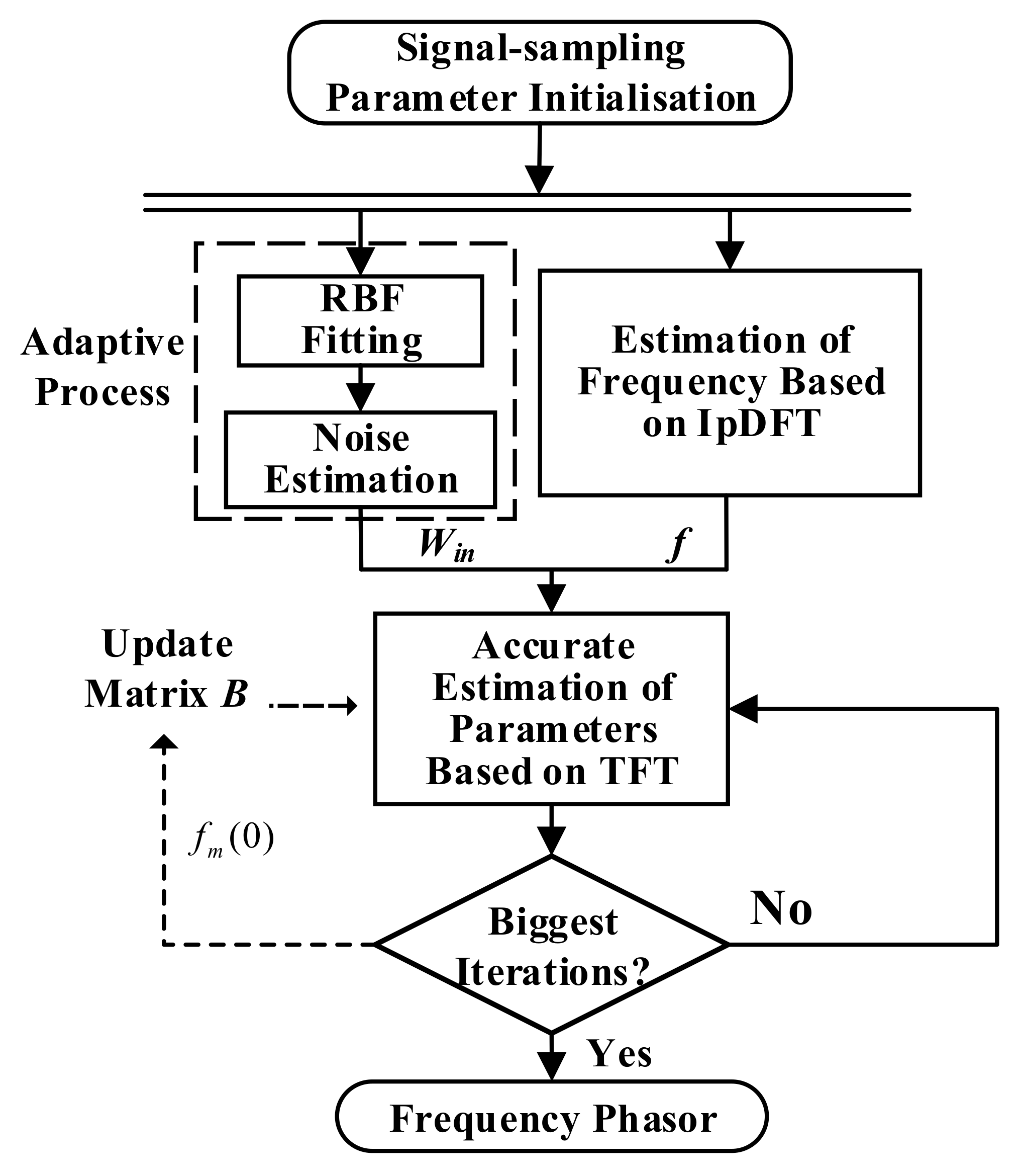
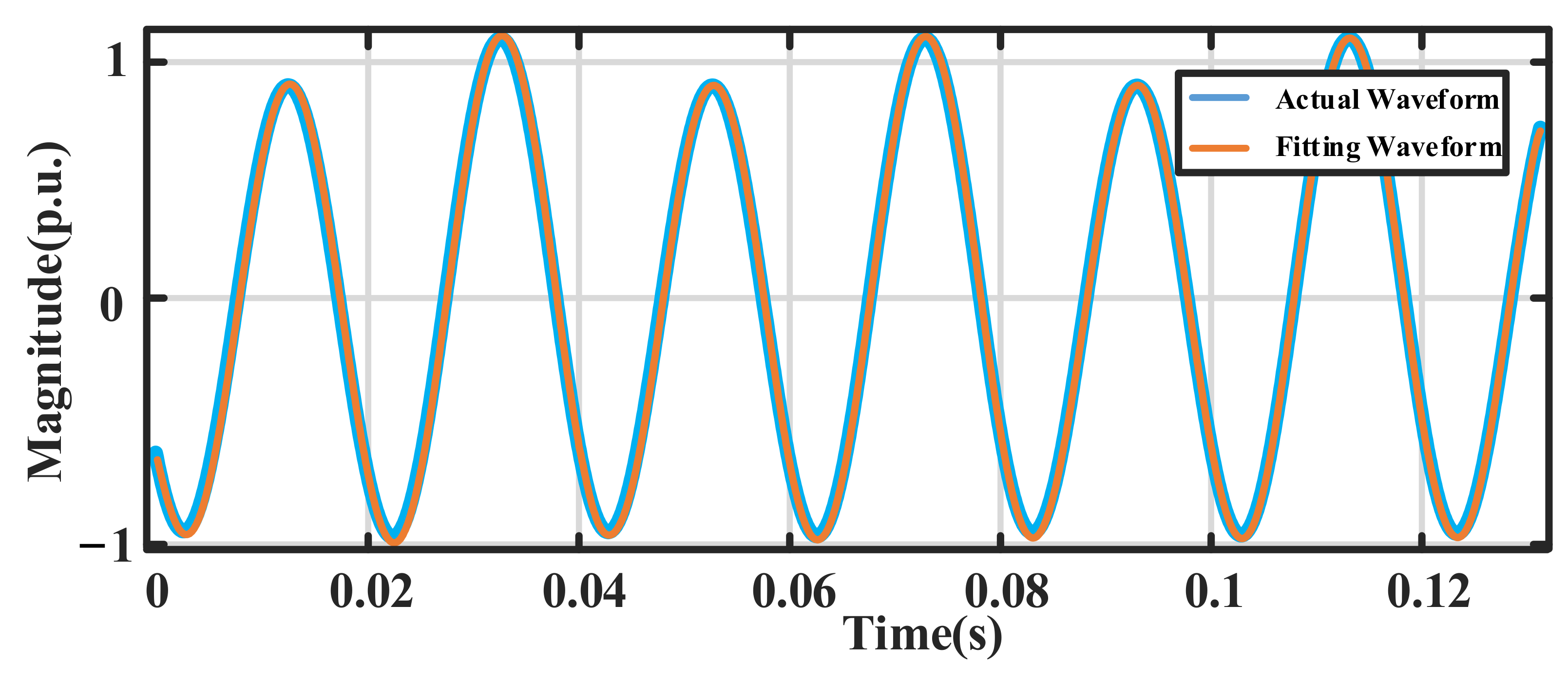
• Fitting signals using RBF neural network algorithms;
• Extracting the noise by comparing the sampled and fitted waveforms, and then estimating the signal-to-noise ratio (SNR);
• Determining the data-window length based on the SNR.

3.2.1. Denoising Using RBF Neural Network

Unlike traditional fitting methods, artificial neural networks have a small dependence on the system’s model and high fault tolerance, making them especially suitable for dealing with complex nonlinear problems and approximating any function; therefore, the neural network method is used to fit the signal. The RBF neural network has a simple structure, high speed, and high fitting accuracy, which is well-suited for denoising [33].

The RBF neural network is a three-layer feedforward network consisting of input, hidden, and output layers. Its structure is shown in Figure 1, where X is the input layer, x_i is the input vector, R is the hidden layer, r_i is the neuron, w_j is the weight vector, and F is the output layer space. An RBF neural network uses a radial basis function as the activation function, which directly maps the input vector space to the hidden layer. Therefore, the hidden layer is nonlinear, whereas the output layer is linear.

Equation (13) shows the key step of the RBF neural network.

$$f\left(x\right)={\displaystyle \sum _{j=1}^v{w}_j}\varphi \left(‖x-x_j‖\right),$$

(13)

where f(x) is the output of the output layer, which can be obtained by the weighted summation of the output of the neurons in the hidden layer; $\varphi \left(‖x-x_j‖\right)$ is the activation function of the hidden layer, mostly a Gaussian function, as shown in (14); and x₀ represents the centre point of the radial basis function.

$$\varphi \left(‖x-x_0‖\right)=\exp \left(-\frac{{‖x-x_0‖}^2}{2{\sigma }^2}\right),$$

(14)

where σ is the variance.

Let the output of the output layer be the expected response of the input vector recorded as

$$F^T=\left(f_1,f_2,\cdots ,f_u\right);$$

(15)

then,

$$\begin{array}{l}{\varphi }_{ij}=\varphi \left(‖x_i-x_j‖\right)\\ W^T=\left(w_1,w_2,\cdots ,w_v\right)\end{array}$$

(16)

Hence, Equation (15) can be rewritten as

$$\underset{\Phi }{\underbrace{\left(\begin{array}{cccc}{\varphi }_{11}& {\varphi }_{12}& \cdots & {\varphi }_{1v}\\ {\varphi }_{21}& {\varphi }_{22}& \cdots & {\varphi }_{2v}\\ ⋮& ⋮& ⋮& ⋮\\ {\varphi }_{u1}& {\varphi }_{u1}& \cdots & {\varphi }_{uv}\end{array}\right)}} \underset{W}{\underbrace{\left(\begin{array}{c}{w}_1\\ w_2\\ ⋮\\ w_v\end{array}\right)}}=\underset{F}{\underbrace{\left(\begin{array}{c}{f}_1\\ f_2\\ ⋮\\ f_u\end{array}\right)}}.$$

(17)

where the signal used for training is the sampled noise signal. From Equation (17), the output layer can be obtained as

$$\Phi W=F.$$

(18)

If Φ is reversible,

$$W={\Phi }^{-1}F.$$

(19)

If Φ is not reversible, W can be solved with pseudo inverse. Because K-means clustering algorithm is efficient and scalable, this paper uses K-means clustering method to adjust the basis function center. The steps are as follows:

• Network initialization: g training samples were randomly selected as the cluster center c_i (i = 1, 2, 3, …, g).
• The input training sample sets are grouped according to the nearest rule: The input samples are assigned to each cluster set $\zeta p(p=1,2,3,\dots ,P)$ according to the Euclidean distance between the input samples and the cluster center.
• Re-adjust cluster centers: Calculate the average value of training samples in each cluster set, i.e., the new cluster center c_i. If the new cluster center no longer changes, the resulting c_i is the final base function center of the RBF neural network. Otherwise, return to the previous step for iteration.

After outputting the result c_i, the weights of the hidden layer and the output layer need to be adjusted by least squares. The adjustment formula is:

$$w=\exp ((\frac{M}{c_{\max }^2})‖x_g-c_{\underset{¯}{n}}‖),$$

(20)

where c_max is the maximum value of the cluster center, g is the number of samples, n is the number of nodes in the hidden layer.

Because RBF neural networks increase computational complexity and reduce real-time performance, long windows should be avoided when fitting. Only one fundamental period of data was used for noise estimation in this study.

3.2.2. Noise Intensity Estimation

The noise data can be obtained by subtracting the original waveform from the waveform fitted by the RBF neural network, and the SNR can be obtained according to Equation (21), with units of dB.

$$SNR=10{\log }_{10}\left(\frac{P_S}{P_N}\right),$$

(21)

where P_S and P_N are the power of the signal and noise, respectively.

3.2.3. Determining the Window Length

When SNR is high, less amount of data is required and vice versa. The number of data used for TFT is determined through trial and error, and authors did a lot of tests to find the optimal window length under different SNRs. It is found that the TFT algorithm needs 5 cycles for the SNR higher than 40 dB and 10 cycles for the SNR lower than 15 dB. For the SNR between 15 and 40, the window length is designed as Equation (22). If the result is decimal, a rounding operation is performed:

$$W_{in}=\left\{\begin{array}{cc}\frac{f_s}{5},& SNR\le 15\\ \left(\frac{195-3\times SNR}{15}\right)\times \frac{f_s}{50},& 15<SNR<40\\ \frac{f_s}{10},& SNR\ge 40\end{array}\right..$$

(22)

The required window length in this study was always between five to ten fundamental cycles for a 50 Hz system. This method slightly reduces the dynamic performance of the algorithm when the SNR is low but significantly improves the accuracy under noisy conditions. Therefore, our method strikes a good balance between dynamic performance and estimation accuracy. Note that the window-length function in Equation (22) can be adjusted according to monitoring needs.

3.3. Flowchart of the Proposed Method

An overall flowchart of the algorithm is shown in Figure 2. First, the order of Taylor expansion and the number of iterations of the TFT are determined; then, fast and noise intensity estimation of the sampling sequence is performed to obtain the initial frequency and window length, respectively. Finally, frequency, amplitude, and phase parameters are calculated through iterations based on the TFT.

4. Simulations Verification

4.1. Performance Assessment Standard

The C37.118.1-2011 IEEE standard [34] was used to evaluate the total vector error (TVE) and frequency error (FE) of the results obtained by different algorithms. The TVE and FE are defined as follows:

$$TVE\left(n\right)=\sqrt{\frac{{\left({\widehat{X}}_{\mathrm{r}}\left(n\right)-X_{\mathrm{r}}\left(n\right)\right)}^2+{\left({\widehat{X}}_{\mathrm{i}}\left(n\right)-X_{\mathrm{i}}\left(n\right)\right)}^2}{{\left(X_{\mathrm{r}}\left(n\right)\right)}^2+{\left(X_{\mathrm{i}}\left(n\right)\right)}^2}},$$

(23)

$$FE=\left|f-\widehat{f}\right|,$$

(24)

where X_r(n) and X_i(n) are the real and imaginary parts of the real value of the phasor at time n, respectively; ${\widehat{X}}_{\mathrm{r}}\left(n\right)$ and ${\widehat{X}}_{\mathrm{i}}\left(n\right)$ are the real and imaginary parts of the estimated phasor at time n, respectively; and f and $\widehat{f}$ are the true and estimated values of the frequency, respectively.

4.2. Simulation Signal Test

The sub-synchronous oscillation is taken as an example to verify the effect of the proposed algorithm. The simulation signal is shown in Equation (25) and 40 dB Gaussian white noise is added. The waveform is shown in Figure 3. The Taylor Fourier is of second order and it is iterated three times.

$$y=\cos (2\pi \times 49.73t+\frac{3}{4}\pi )+0.1\times e^{0.1t}\cos (2\pi \times 24t+\frac{1}{3}\pi )$$

(25)

The window length corresponding to an SNR of 40 dB was five fundamental cycles, and the fitting results are shown in Figure 4. The overall phasor error percentage and frequency error of the fundamental frequency components are 0.17% and 0.003 Hz, respectively, and those for the SSO components are 1.78% and 0.35 Hz, respectively.

To further verify the effect of the proposed method under complex working conditions, the PMU test standard in the C37.118.1-2011 IEEE standard was applied and the following simulation was designed: the noise level in each simulation was varied from 15 to 60 dB.

(1)

Amplitude-modulation dynamics

In real situations, the amplitude variation of the SSO may be complicated by various factors. In this example, the amplitude is modulated by a sinusoidal variation, and the modulation level of the amplitude is set to 10%. The signal model is given by Equation (26), and the results are shown in Figure 5.

$$\begin{array}{ll}y=& \cos (2\pi \times 49.73t+3\pi /4)+\\ & 0.1\times \left(1+0.1\times \cos (2\pi t)\right)\cos (2\pi \times 24t+\pi /3)\end{array}$$

(26)

(2)

Frequency-ramp dynamics

In an actual oscillation accident, the SSO frequency may drop or climb continuously; therefore, the slope function is taken as an example to simulate, and the signal model is as shown in Equation (27). The frequency component of the SSO component was superimposed with a linear term of 10 t, and the simulation results are shown in Figure 6.

$$\begin{array}{ll}y=& \cos (2\pi \times 49.73t+3\pi /4)+\\ & 0.1\cos (2\pi \times 24t+\pi /3+10\pi t^2)\end{array}$$

(27)

(3)

Frequency-modulation dynamics

In an actual power system, the change in the SSO frequency is not always linear, and the frequency can be sinusoidally modulated. The modulation signal is shown in Equation (28), where the frequency is superimposed with the sine term −10 sin (2π × 0.1 t). The simulation results are shown in Figure 7.

$$\begin{array}{ll}y=& \cos (2\pi \times 49.73t+3\pi /4)+\\ & 0.1\cos (2\pi \times 24t+\pi /3+100\cos (2\pi \times 0.1t))\end{array}$$

(28)

(4)

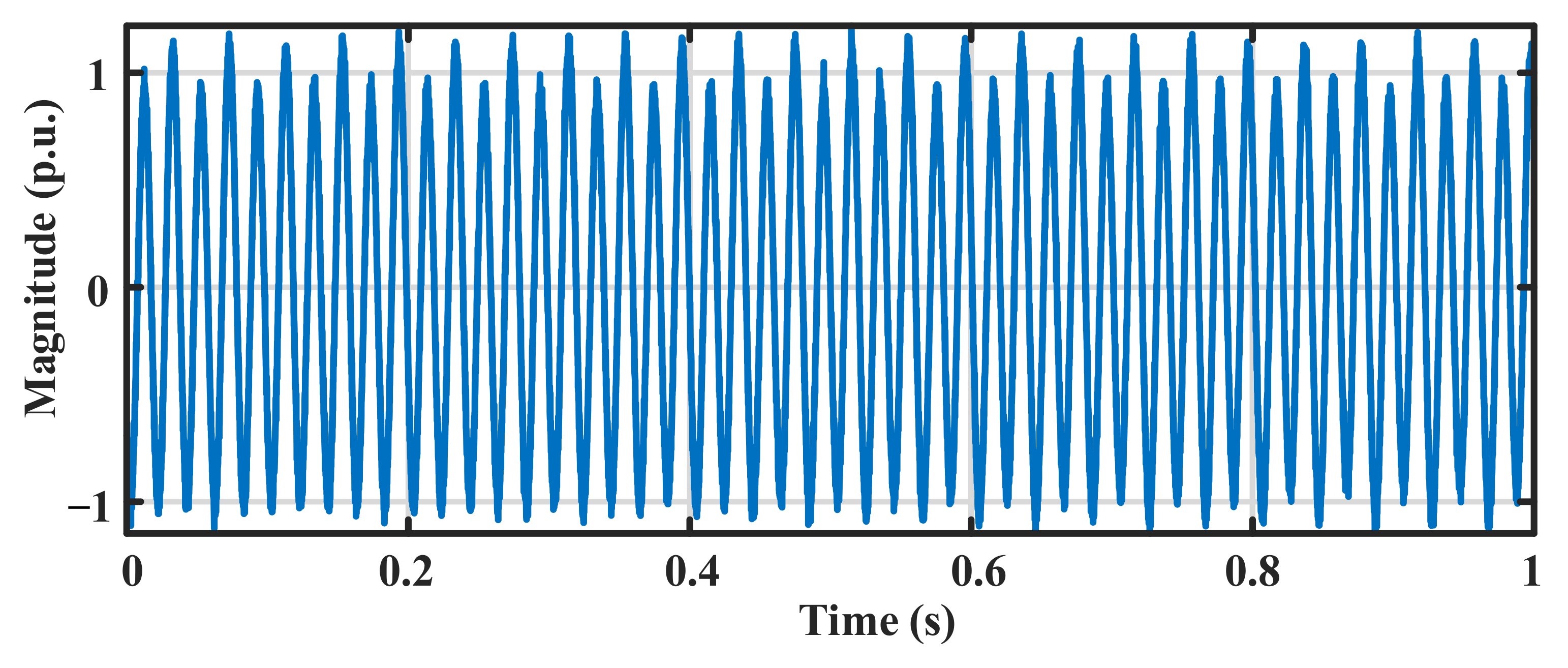
Multi-mode wideband oscillations

Multiple oscillation components may exist in wideband oscillation; for example, there may be harmonics and interharmonics simultaneously, and the dynamic process of each signal component is different, complicating the working conditions and increasing the requirements of the monitoring algorithm. The simulation signal of this example is shown in Equation (29) and the specific parameters are shown in

Table 1. Signal Parameters.

Serial Number	p.u.	Rad
1	0.1e0.1t	π/3 + 100 cos (0.2πt)
2	1 + 5/12 cos (0.24πt)	0.75π + πt2
3	0.1e0.1t	−100 cos (0.2πt)
4	0.1	7π/12 + 5πt2
5	0.1e0.15t	7π/36 + 10πt2
6	0.1	5π/3 + 17πt2

. The simulation results are displayed in Figure 8.

$$\begin{array}{ll}y=& A_1\cos (2\pi \times 24t+{\varphi }_1(t))+A_2\cos (2\pi \times 49.73t+{\varphi }_2(t))+\\ & A_3\cos (2\pi \times 76t+{\varphi }_3(t))+A_4\cos (2\pi \times 248.65t+{\varphi }_4(t))+\\ & A_5\cos (2\pi \times 521t+{\varphi }_5(t))+A_6\cos (2\pi \times 845.41t+{\varphi }_6(t))\end{array}$$

(29)

4.3. Discussion of Algorithms

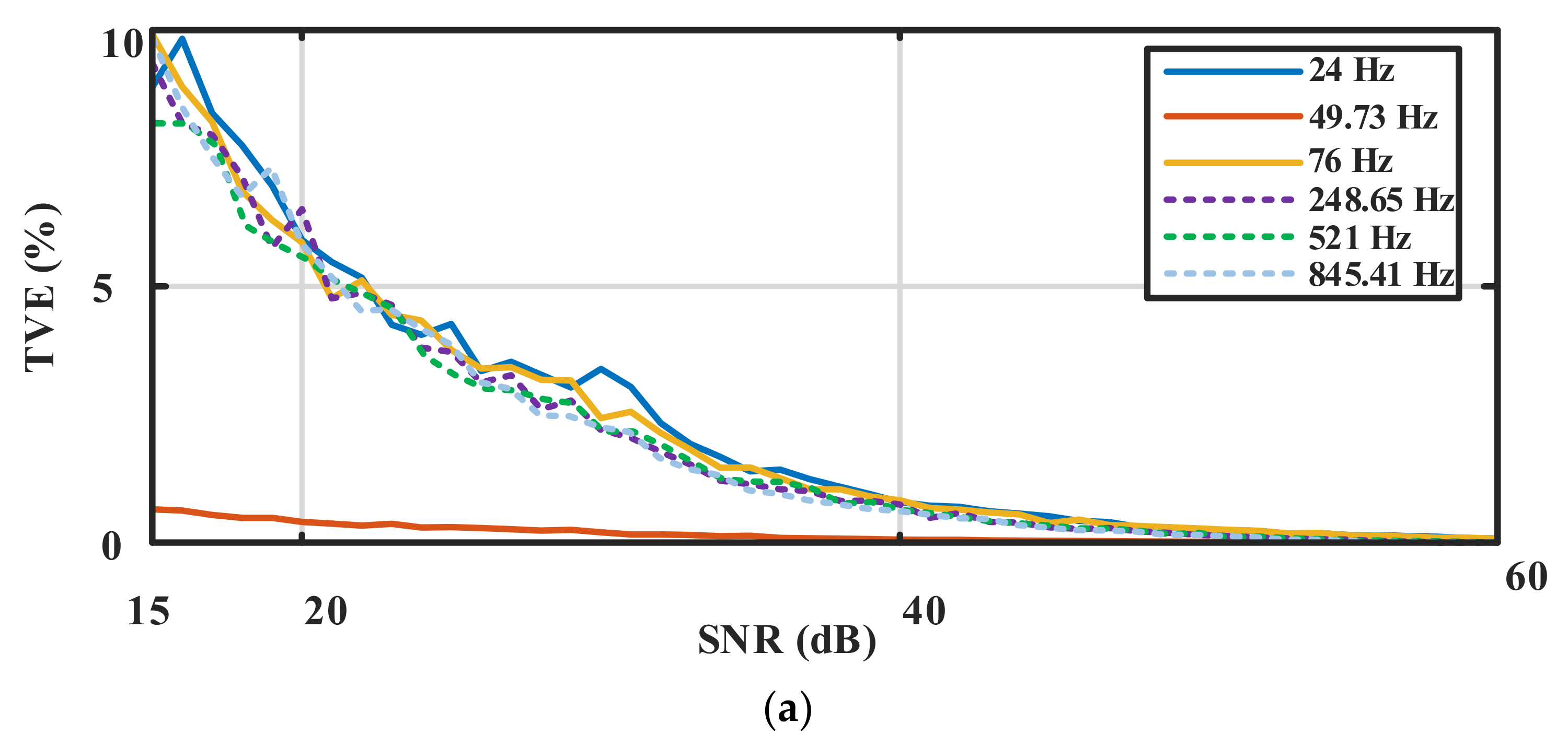
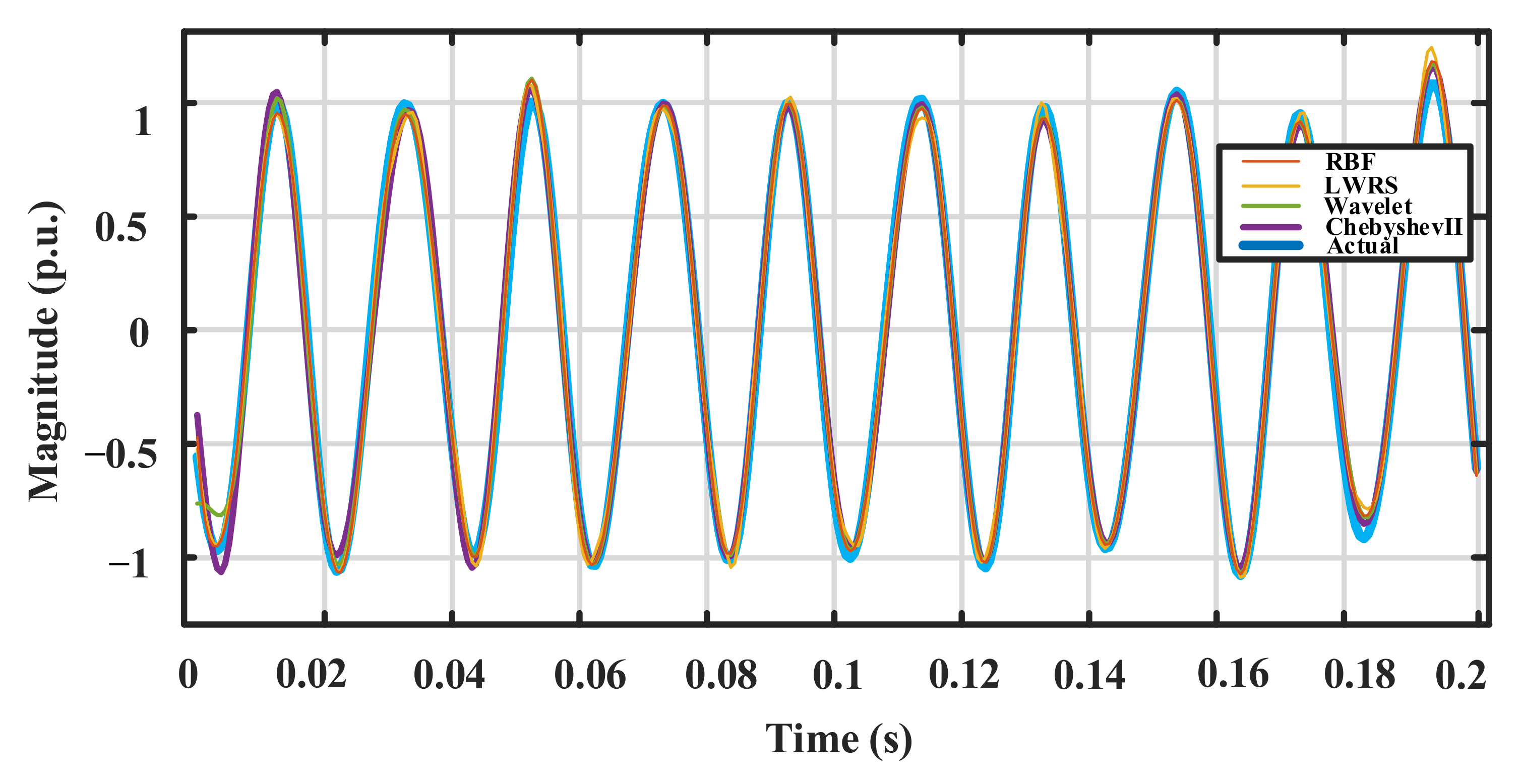
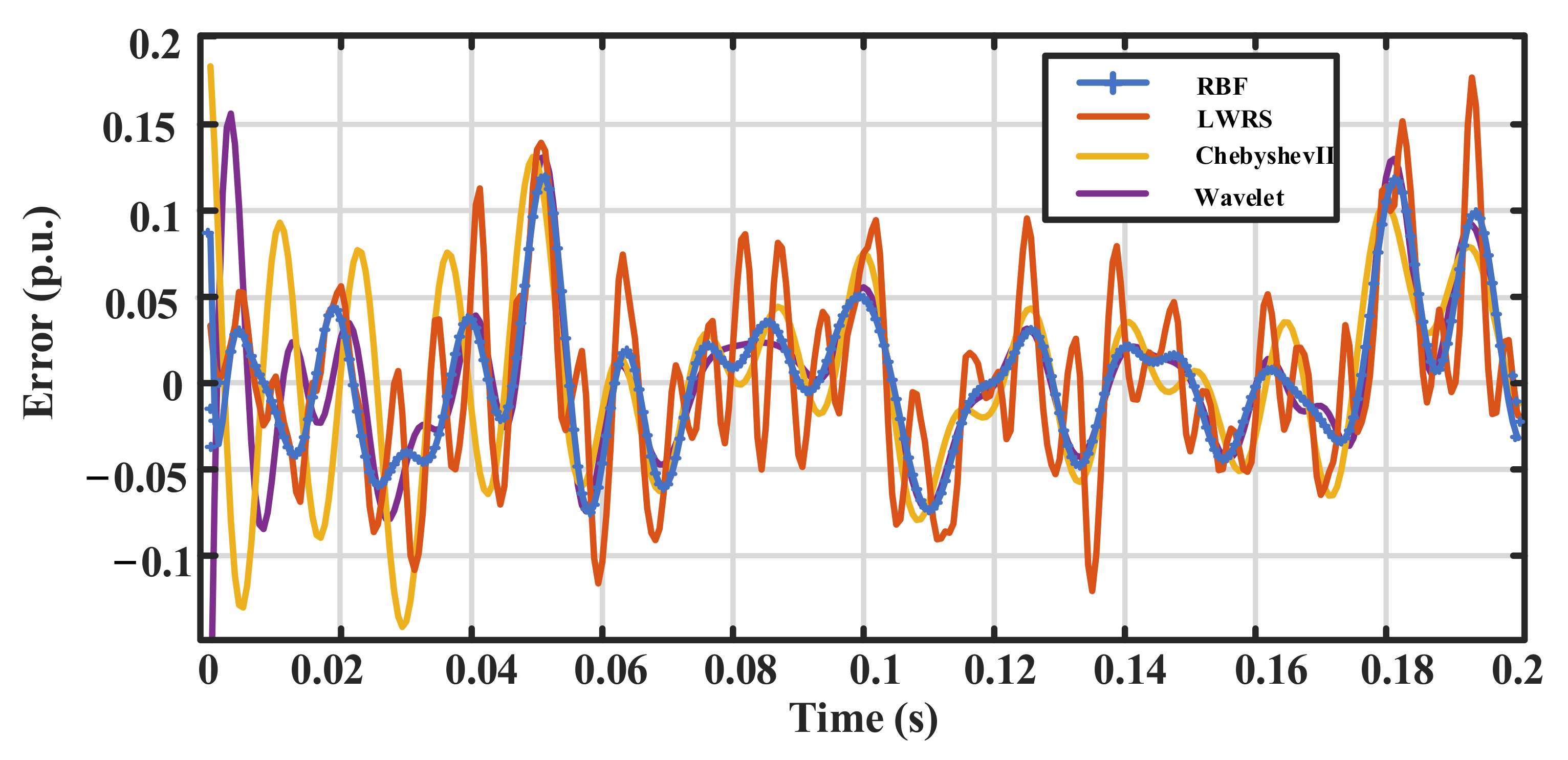
• The simulation results show that the proposed algorithm has superior dynamic performance, as it can cope with dynamic change process and maintains its accuracy under high noise levels. Theoretically, the dynamic performance improves with the Taylor expansion order, but the higher expansion order increases the computation cost.
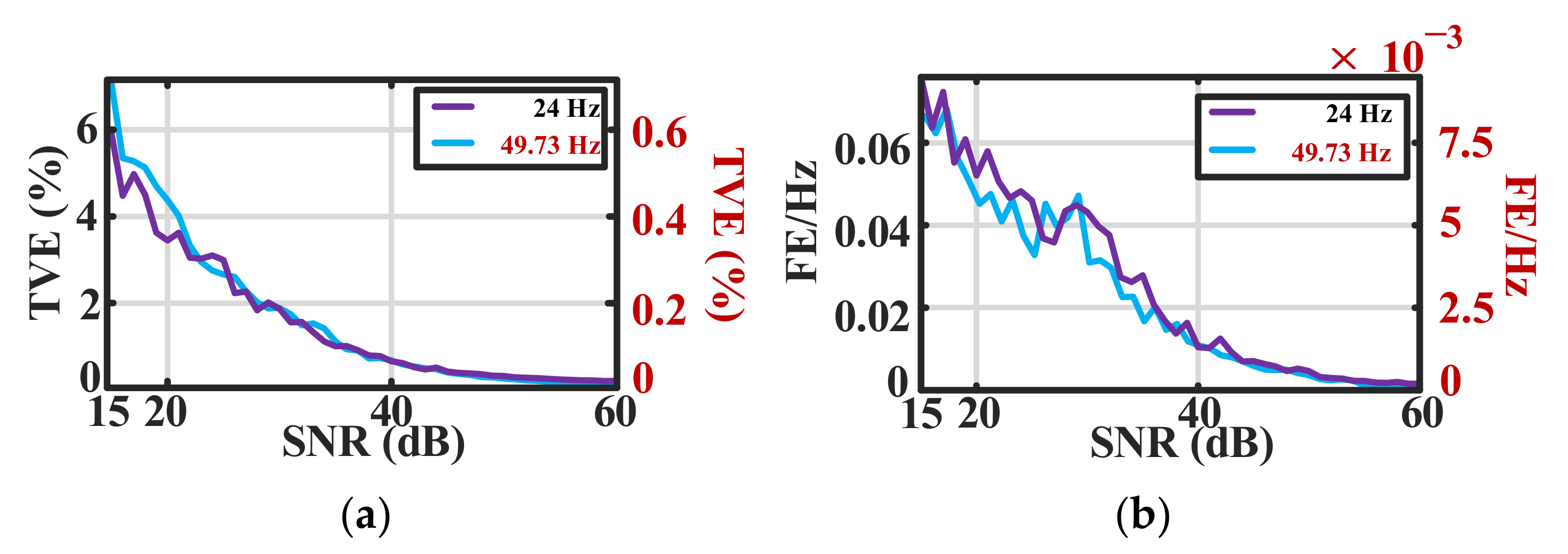
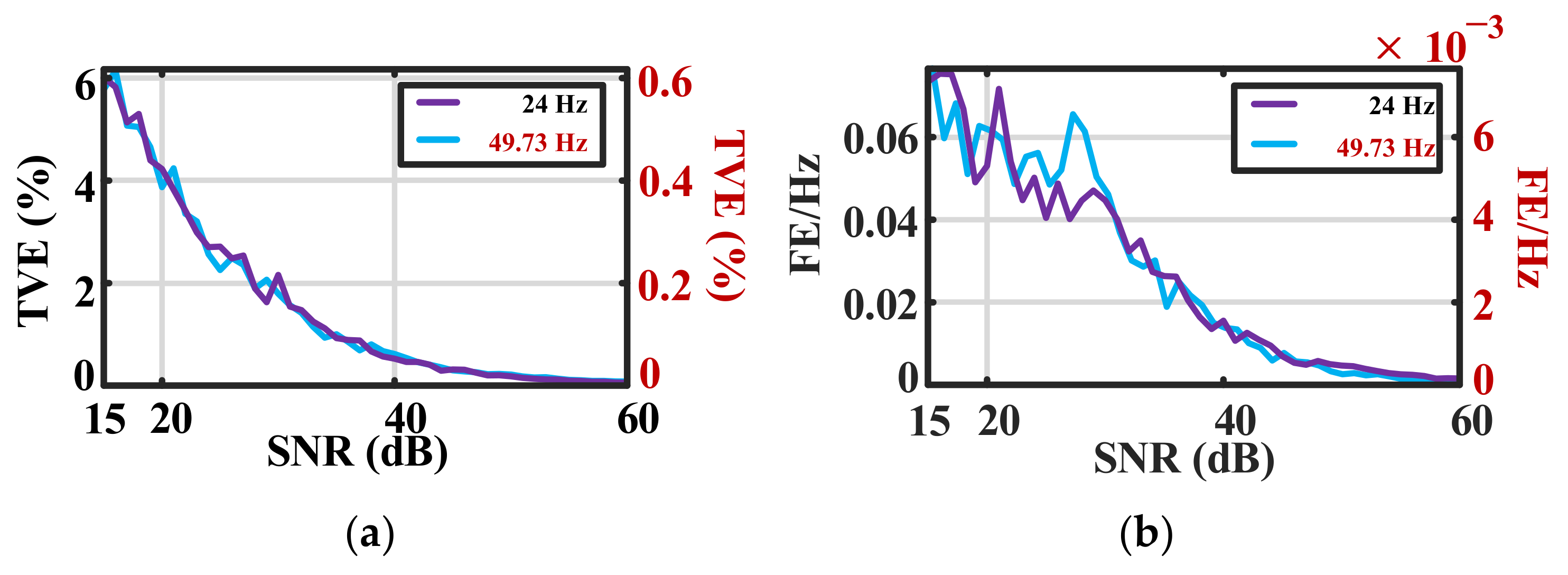
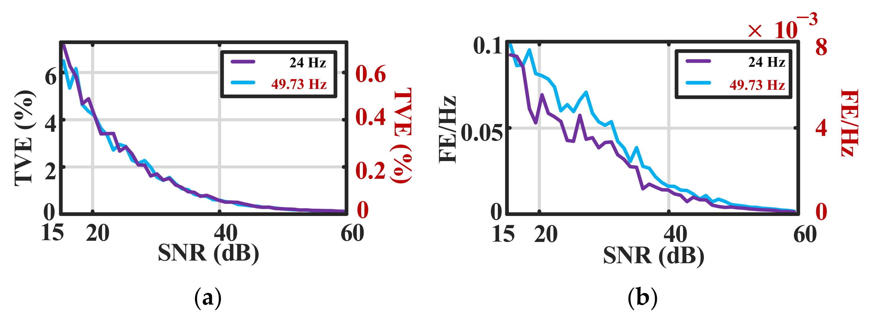
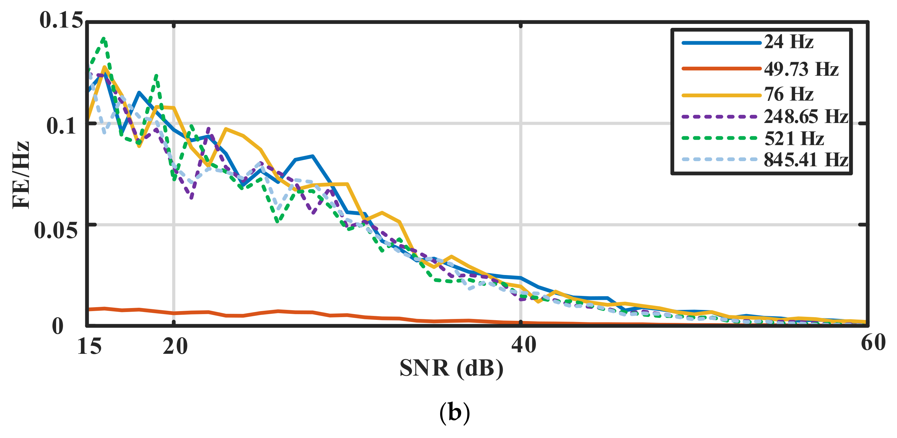
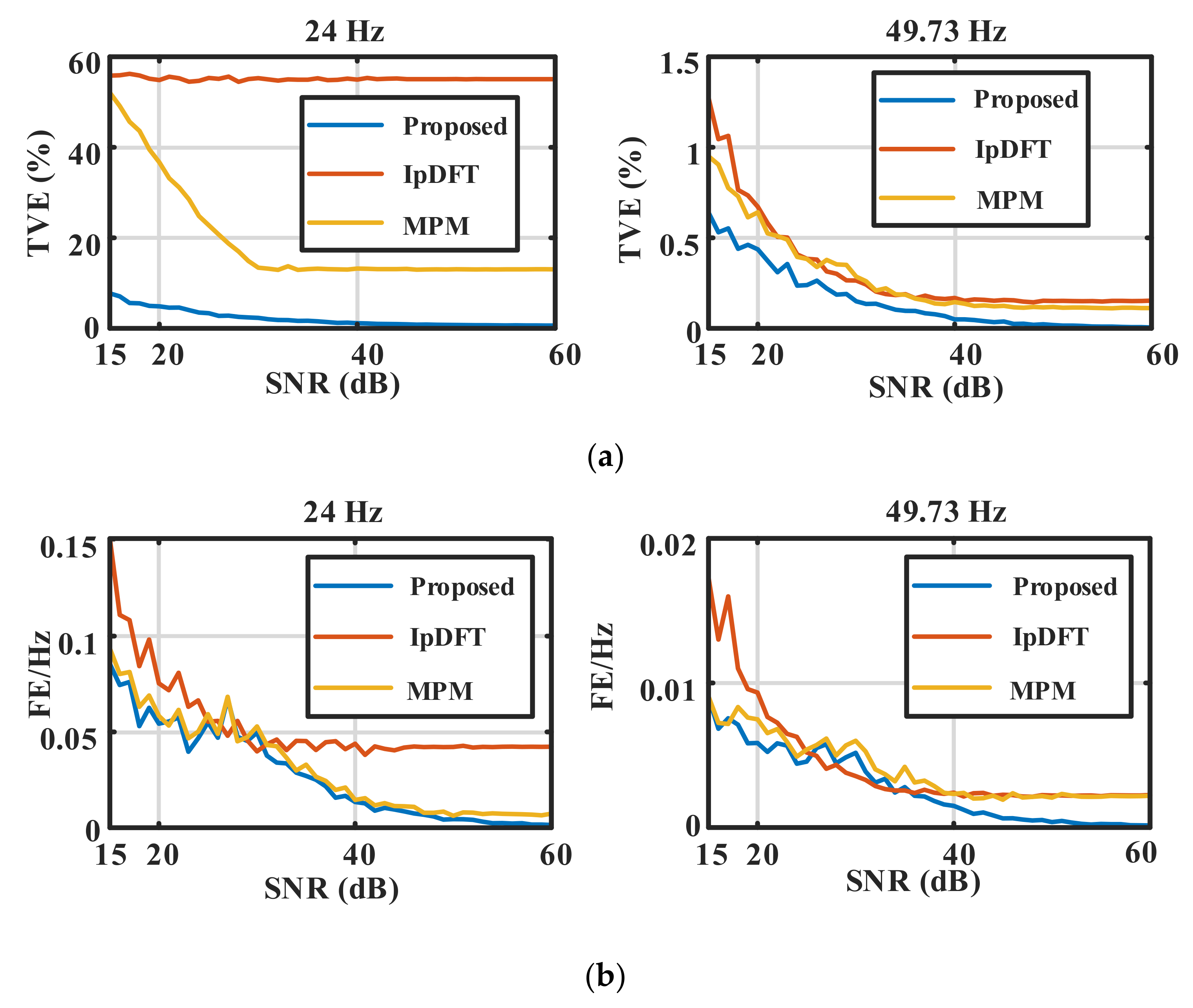
• The phasor and frequency errors of the power frequency component are much smaller than those of the other signal components because the power frequency component has a larger amplitude and is less affected by noise. According to the measurement standards for power frequency phasors given in IEEE Std. C37.118.1-2011, the maximum overall phasor error and maximum frequency error are 1% and 0.01 Hz, respectively. A combination of Figure 5, Figure 6, Figure 7 and Figure 8 reveals that the proposed algorithm fully satisfies this requirement.
• The TFT algorithm is extremely dependent on the initial frequency, and the oscillation signal may be too noisy to be identified by the IpDFT algorithm at the early stage of oscillation, which may collapse the TFT algorithm. Therefore, the sampling signal can be pre-processed using the proposed algorithm.
• The data-window length also has a significant influence on the TFT algorithm. If the dynamic performance needs to be improved, specific choices can be made according to scenario requirements, and accuracy can be sacrificed to further reduce the window length.

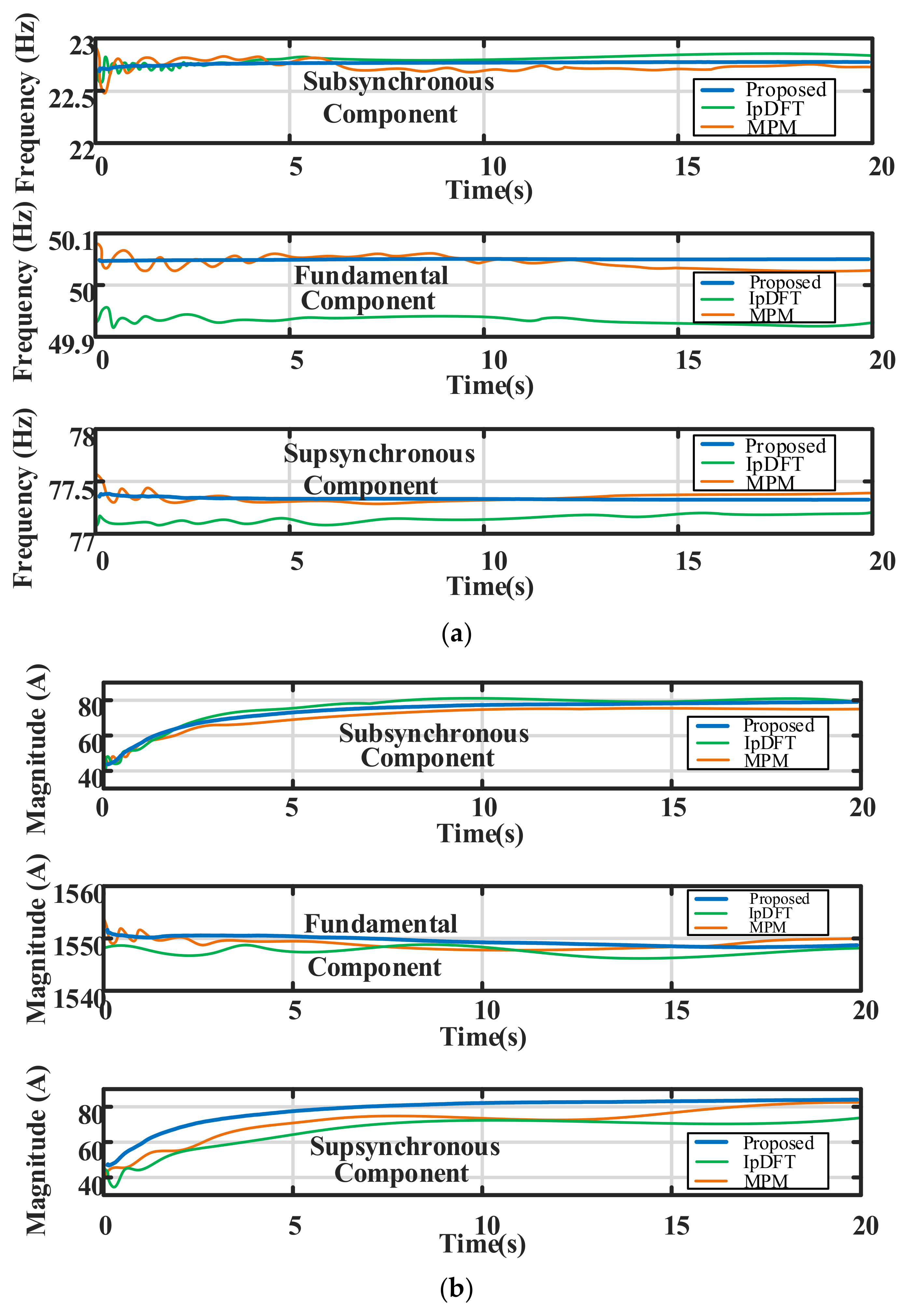
4.4. Comparison of Algorithms

In this section, the proposed algorithm is compared with the IpDFT and the matrix pencil method (MPM). The window length of the MPM was consistent with the window length of the proposed algorithm, and singular value decomposition was performed. Taking the ramp change in the SSO frequency as a comparison example, the simulation settings are consistent with Equation (27), and the comparison results are shown in Figure 9.

The comparison results show that when identifying the sub-synchronisation components with nonlinear frequency changes, the error of the identification results of the IpDFT and MPM is larger because the two algorithms average the oscillation parameters in the window. Therefore, these algorithms are more suitable for linearly changing signals but cannot be adapted to nonlinear signals. In the identification of steady-state power frequency components, the identification results of the two are inferior to those of the proposed algorithm, mainly because noise and the data-window length have a greater impact on the IpDFT and MPM.

To show the fitting effect of the RBF neural network, this study compares locally weighted regression smoothing (LWRS), the Chebyshev II digital filter, and the wavelet algorithm with the RBF neural network. The signal model is as follows:

$$\begin{array}{ll}y=& \cos (2\pi \times 49.73t+3\pi /4+10\pi t^2)+\\ & 0.1e^{0.1t}\cos (2\pi \times 24t+\pi /3)+0.15e^{0.2t}\cos (2\pi \times 76t)\end{array}$$

(30)

where 15 dB of white Gaussian noise is added to the simulation signal. In addition, for observation convenience, the sampling rate was reduced to 1600 Hz. The fitting order of the LWRS algorithm is the second order. Additionally, the window length is 15 cycles, the passband frequency of the Chebyshev II filter is 80 Hz, the passband ripple is 0.1 dB, the stopband frequency is 81 Hz, and the stopband attenuation is 80 dB. The wavelet algorithm adopts the dmey wavelet, and the number of decomposition layers is set to 3. The fitting comparison is shown in Figure 10, and the error comparison is depicted in Figure 11.

The fitting results and the error comparison chart show that the fitting error of the RBF neural network is smaller, the SNR estimation is more accurate, and there is no complicated parameter setting process.

The above test was conducted in the MATLAB platform (MATLAB version: 697 R2016(a), PC with 8.00 GB RAM and 3.60 GHz Intel(R) Core 698 (TM) CPU) manufactured by Intel Corporation in Santa Clara, USA. When the signal contains a small number of harmonic or interharmonic signals, the computational efficiency of the proposed algorithm is high. For example, when the signal contains only sub-synchronous oscillation components, the calculation time of the proposed algorithm is about 0.06 s, whereas the calculation time of the MPM algorithm and the IpDFT algorithm is about 0.25 s and 0.002 s, respectively. However, when there are a large number of harmonics or interharmonics in the signal, such as six oscillation components, the calculation time of the proposed algorithm becomes 0.11 s, while the calculation time of the MPM algorithm and the IpDFT algorithm is not changed. The calculation efficiency of the proposed method is related to the signal complexity, and the main reason is that the dimension of matrix B composed of Taylor Fourier basis vectors in TFT algorithm is greatly increased with the number of oscillating components. As a result, calculating the solution of vector P will be very time-consuming.

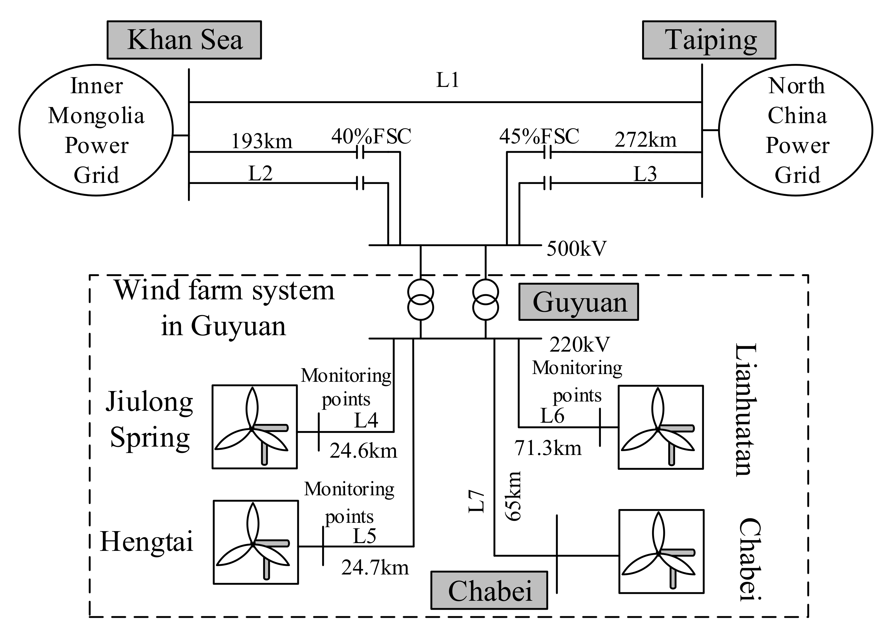
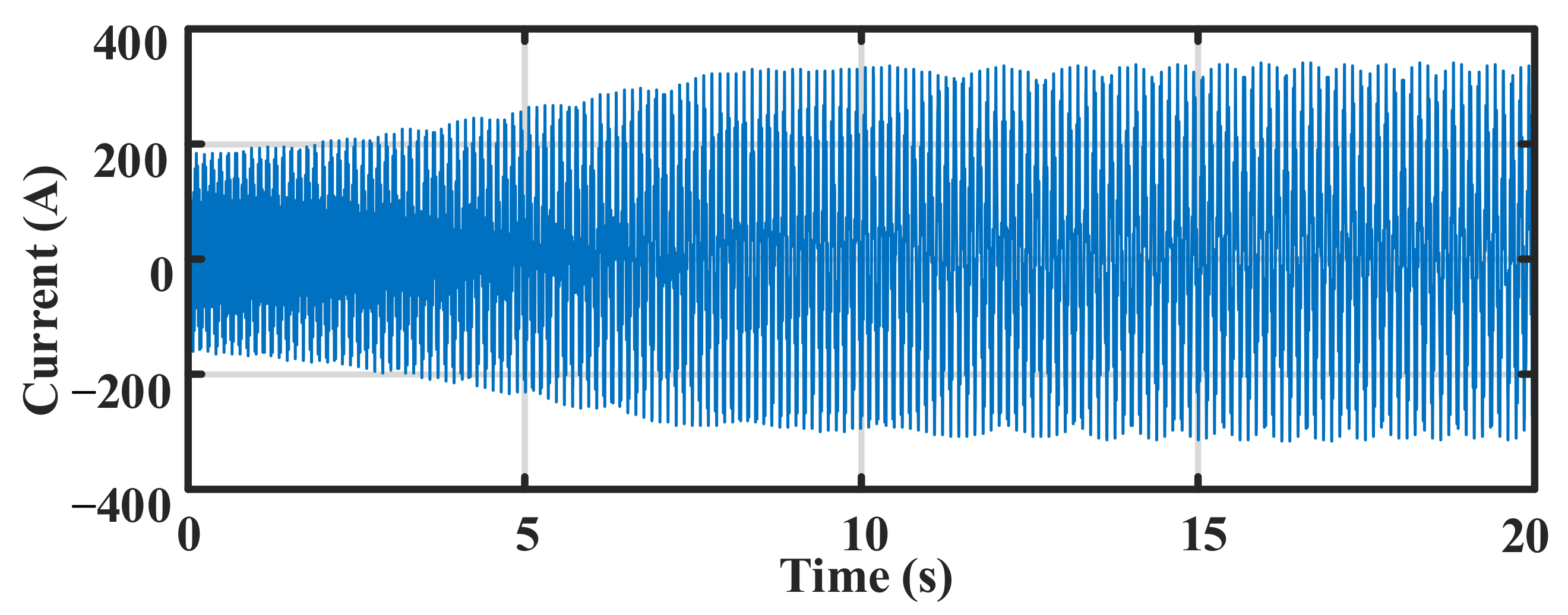
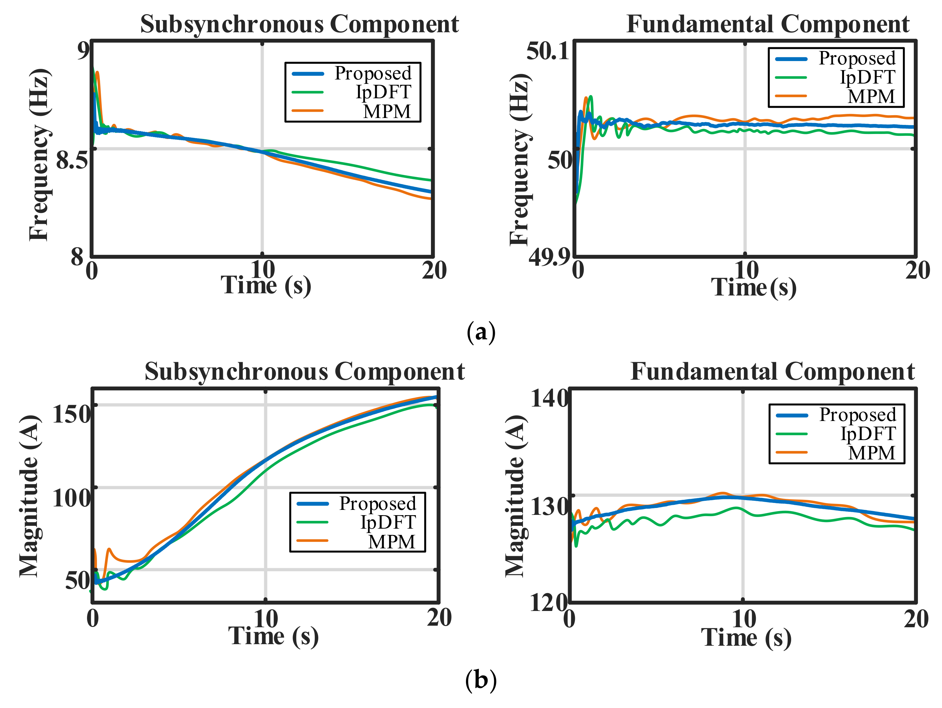
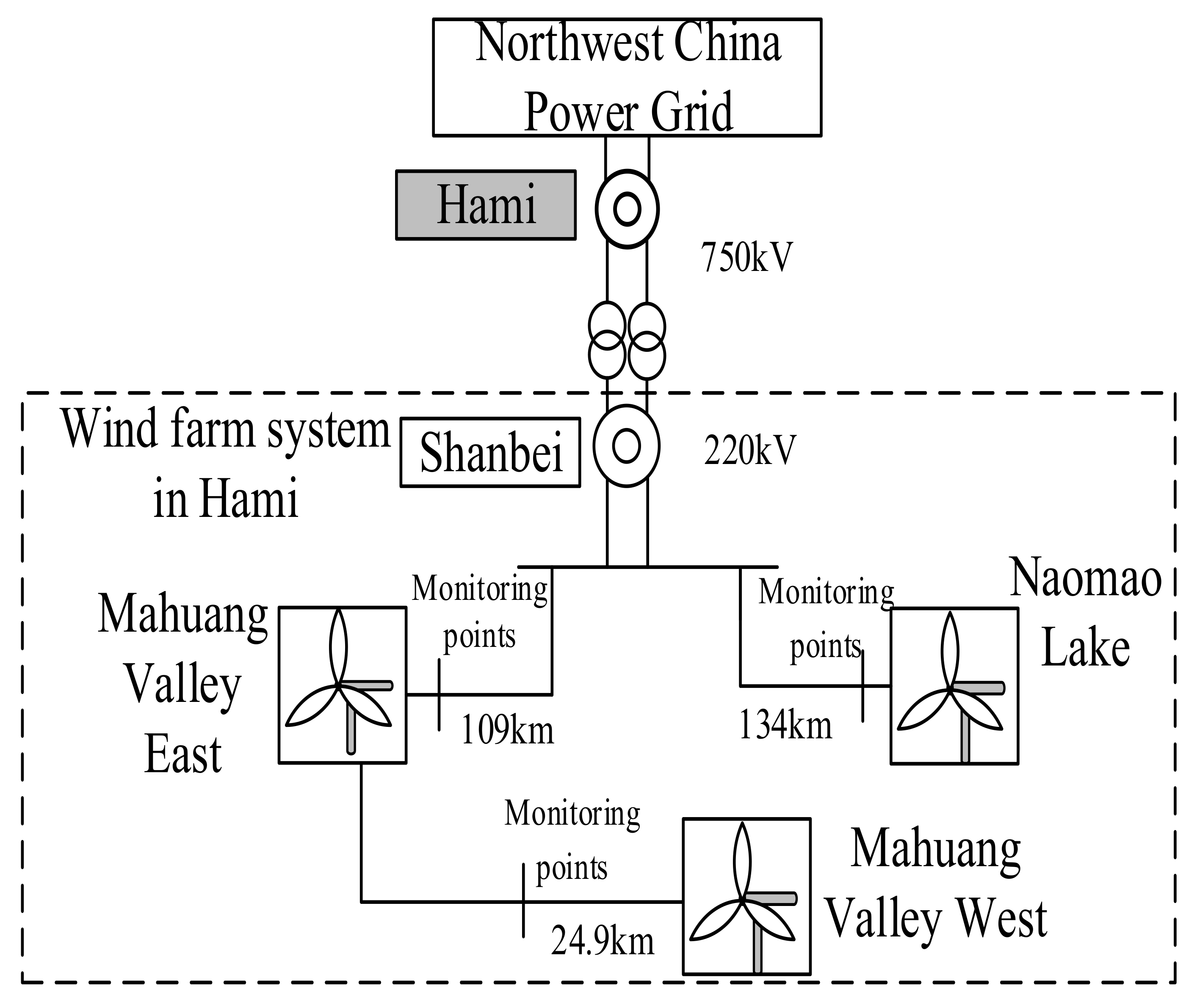
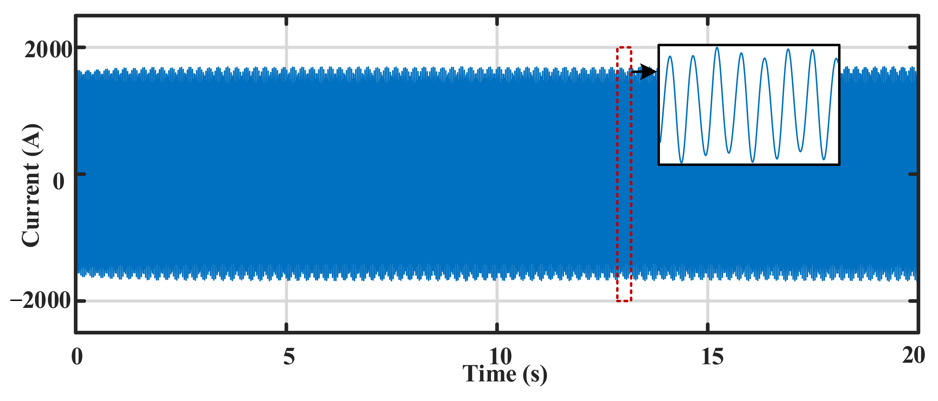
5. Field Data Verification

In this section, the performance of the proposed method is verified and compared with IpDFT and MPM using the real-life wideband oscillation data collected from Guyuan, Hebei, and Hami, Xinjiang. The power grid structure of Guyuan is shown in Figure 12. The current at the Guyuan is shown in Figure 13, and the identification results are presented in Figure 14. The power grid structure of Hami is shown in Figure 15. The current at the Hami is shown in Figure 16, and the identification results are presented in Figure 17.

According to the RBF fitting results, the noise intensities at the Guyuan and Hami stations are approximately 30 dB and 55 dB, respectively. However, because of the low sampling rates of the fault recorders of the Guyuan and Hami stations (only 3200 Hz and 1200 Hz, respectively), the data-window length slightly increases to 10 cycles.

The identification results show that only sub-synchronous oscillation occurred in Guyuan, while the Hami station had sub- and super-synchronous components at the same time. It can be seen that the performance of the proposed method is close to MPM, while the result obtained by IpDFT has large differences with the other two. Comparatively, the frequency and the magnitude identified by the proposed method are most smooth, which indicates a reliable identification. According to post accident analysis, the causes of oscillation accidents in Guyuan and Hami are different. The former one is caused by the interaction between the doubly fed induction generator and the fixed series capacitor, while the latter is caused by the control interaction between the direct-drive wind turbine generator and the weak system. However, regardless of the type of oscillation accidents, the amplitude of the oscillation increases rapidly in a short time, which may endanger the system’s safe and stable operation.

6. Conclusions

This paper presents an improved TFT method for wideband oscillation monitoring with an adaptive window length. First, DFT was used to obtain the initial frequency parameters, and the RBF neural network was used for fitting and denoising to obtain the noise intensity and adaptively determine the data-window length. Finally, TFT was used to iteratively extract the oscillation parameters based on the obtained window length and the initial frequency.

The proposed method has been verified by extensive field data collected from real-world incidents. The results show that the RBF neural network algorithm has a good fitting performance and the dynamic performance of TFT under adaptive window length is satisfactory. When the SNR is 45 dB, the maximum overall phasor error and the maximum frequency error are 1% and 0.01 Hz, respectively. The proposed method is not limited to oscillation monitoring but can also be extended to other fields such as power quality and transient analysis. How to reduce the computation burden and realize the real-time monitoring will be the focus of the future research.

References

1. Basu, J.B.; Dawn, S.; Saha, P.K.; Chakraborty, M.R.; Ustun, T.S. A Comparative Study on System Profit Maximization of a Renewable Combined Deregulated Power System. Electronics 2022, 11, 2857. [Google Scholar] [CrossRef]
2. Alamri, B.; Hossain, M.A.; Asghar, M.J. Electric Power Network Interconnection: A Review on Current Status, Future Prospects and Research Direction. Electronics 2021, 10, 2179. [Google Scholar]
3. Hussain, S.M.S.; Nadeem, F.; Aftab, M.A.; Ali, I.; Ustun, T.S. The Emerging Energy Internet: Architecture, Benefits, Challenges, and Future Prospects. Electronics 2019, 8, 1037. [Google Scholar] [CrossRef] [Green Version]
4. Xie, X.; Zhan, Y.; Shair, J.; Ka, Z.; Chang, X. Identifying the Source of Subsynchronous Control Interaction via Wide-Area Monitoring of Sub/Super-Synchronous Power Flows. IEEE Trans. Power Deliv. 2020, 35, 2177–2185. [Google Scholar] [CrossRef]
5. Zhan, Y.; Xie, X.; Liu, H.; Liu, H.; Li, Y. Frequency-Domain Modal Analysis of the Oscillatory Stability of Power Systems With High-Penetration Renewables. IEEE Trans. Sustain. Energy 2019, 10, 1534–1543. [Google Scholar] [CrossRef]
6. Xu, S.; Wang, Y.; Xiao, X.; Wu, J.; Lv, W. Non-Characteristic Harmonic Resonance in LCC-HVDC Terminals: A Practical Case Study. Int. Trans. Electr. Energ. Syst. 2021, 31, e12743. [Google Scholar] [CrossRef]
7. Adams, J.; Pappu, V.A.; Dixit, A. ERCOT experience screening for Sub-Synchronous Control Interaction in the vicinity of series capacitor banks. In Proceedings of the 2012 IEEE Power and Energy Society General Meeting, San Diego, CA, USA, 22–26 July 2012; pp. 1–5. [Google Scholar]
8. Wang, L.; Xie, X.; Jiang, Q.; Liu, H.; Li, Y.; Liu, H. Investigation of SSR in Practical DFIG-Based Wind Farms Connected to a Series-Compensated Power System. IEEE Trans. Power Syst. 2015, 30, 2772–2779. [Google Scholar] [CrossRef]
9. Liu, H.; Xie, X.; He, J.; Xu, T.; Yu, Z.; Wang, C.; Zhang, C. Subsynchronous Interaction Between Direct-Drive PMSG Based Wind Farms and Weak AC Networks. IEEE Trans. Power Syst. 2017, 32, 4708–4720. [Google Scholar] [CrossRef]
10. Li, W.; Wang, Q. Stochastic production simulation for generating capacity reliability evaluation in power systems with high renewable penetration. Energy Convers Econ. 2020, 1, 210–220. [Google Scholar] [CrossRef]
11. Qi, J.; Tang, F.; Xie, J.; Li, X.; Wei, X.; Liu, Z. Research on Frequency Response Modeling and Frequency Modulation Parameters of the Power System Highly Penetrated by Wind Power. Sustainability 2022, 14, 7798. [Google Scholar] [CrossRef]
12. Corsi, S.; Taranto, G.N. A Real-Time Voltage Instability Identification Algorithm Based on Local Phasor Measurements. IEEE Trans. Power Syst. 2008, 23, 1271–1279. [Google Scholar] [CrossRef]
13. Wang, Y.; Jiang, X.; Xie, X.; Yang, X.; Xiao, X. Identifying Sources of Subsynchronous Resonance Using Wide-Area Phasor Measurements. IEEE Trans. Power Deliv. 2021, 36, 3242–3254. [Google Scholar] [CrossRef]
14. Li, H.; Abdeen, M.; Chai, Z.; Kamel, S.; Xie, X.; Hu, Y.; Wang, K. An Improved Fast Detection Method on Subsynchronous Resonance in a Wind Power System With a Series Compensated Transmission Line. IEEE Access. 2019, 7, 61512–61522. [Google Scholar] [CrossRef]
15. Chen, W.; Wang, D.; Xie, X.; Ma, J.; Bi, T. Identification of Modeling Boundaries for SSR Studies in Series Compensated Power Networks. IEEE Trans. Power Syst. 2017, 32, 4851–4860. [Google Scholar] [CrossRef]
16. Appasani, B.; Mohanta, D.K. A review on synchrophasor communication system: Communication technologies, standards and applications. Prot. Control Mod. Power Syst. 2018, 3, 37. [Google Scholar] [CrossRef] [Green Version]
17. Zhao, J.; Zhang, Y.; Zhang, P.; Jin, X.; Fu, C. Development of a WAMS based test platform for power system real time transient stability detection and control. Prot. Control Mod. Power Syst. 2016, 1, 6. [Google Scholar] [CrossRef] [Green Version]
18. Ling, W.; Jie, W.; Li, W.; Chao, S.; Kaipei, L. The 7-terms Harris window and interpolated FFT harmonic analysis method for electrified railway. In Proceedings of the 2014 International Conference on Information Science, Electronics and Electrical Engineering, Sapporo, Japan, 26–28 April 2014; Volume 1, pp. 18–23. [Google Scholar]
19. Derviškadić, A.; Romano, P.; Paolone, M. Iterative-interpolated DFT for synchrophasor estimation: A single algorithm for P- and M-class compliant PMUs. IEEE Trans Instrum Meas. 2018, 67, 547–558. [Google Scholar] [CrossRef] [Green Version]
20. Shiri, F.; Mohammadi-ivatloo, B. Identification of inter-area oscillations using wavelet transform and phasor measurement unit data. Int. Trans. Electr. Energ. Syst. 2015, 25, 2831–2846. [Google Scholar] [CrossRef]
21. Rana, M.J.; Alam, M.S.; Islam, M.S. Continuous wavelet transform based analysis of low frequency oscillation in power system. In Proceedings of the 2015 International Conference on Advances in Electrical Engineering (ICAEE), Dhaka, Bangladesh, 17–19 December 2015; pp. 320–323. [Google Scholar]
22. Laila, D.S.; Messina, A.R.; Pal, B.C. A Refined Hilbert–Huang Transform with Applications to Interarea Oscillation Monitoring. IEEE Trans. Power Syst. 2009, 24, 610–620. [Google Scholar] [CrossRef] [Green Version]
23. Andrade, M.A.; Messina, A.R.; Rivera, C.A.; Olguin, D. Identification of instantaneous attributes of torsional shaft signals using the Hilbert transform. IEEE Trans. Power Syst. 2004, 19, 1422–1429. [Google Scholar] [CrossRef]
24. Ray, P.K.; Subudhi, B. Ensemble-Kalman-filter-based power system harmonic estimation. IEEE Trans Instrum Meas. 2012, 61, 3216–3224. [Google Scholar] [CrossRef]
25. Yu, K.K.C.; Watson, N.R.; Arrillaga, J. An adaptive Kalman filter for dynamic harmonic state estimation and harmonic injection tracking. IEEE Trans. Power Deliv. 2005, 20, 1577–1584. [Google Scholar] [CrossRef]
26. Jun, W. Feature extraction of localized scattering centers using the modified TLS-Prony algorithm and its applications. J. Syst. Eng. Electron. 2002, 13, 31–39. [Google Scholar]
27. CGrund, E.; Paserba, J.J.; Hauer, J.F.; Nilsson, S.L. Comparison of Prony and eigenanalysis for power system control design. IEEE Trans. Power Syst. 1993, 8, 964–971. [Google Scholar] [CrossRef]
28. Wang, Y.; Yang, H.; Xie, X.; Yang, X.; Chen, G. Real-Time Subsynchronous Control Interaction Monitoring using Improved Intrinsic Time-Scale Decomposition. J. Mod. Power Syst. Clean Energy 2022, 1–11. [Google Scholar] [CrossRef]
29. de la O Serna, J.A. Dynamic phasor estimates for power system oscillations. IEEE Trans Instrum. Meas. 2007, 56, 1648–1657. [Google Scholar] [CrossRef]
30. Chen, L.; Zhao, W.; Wang, F.; Wang, Q.; Huang, S. An interharmonic phasor and frequency estimator for subsynchronous oscillation identification and monitoring. IEEE Trans Instrum. Meas. 2019, 68, 1714–1723. [Google Scholar] [CrossRef] [Green Version]
31. Zhang, H.; Jin, Z.; Terzija, V. An adaptive decomposition scheme for wideband signals of power systems based on the modified robust regression smoothing and Chebyshev-II IIR filter bank. IEEE Trans. Power Deliv. 2019, 34, 220–230. [Google Scholar] [CrossRef]
32. Xu, S.; Wang, Y.; Xiao, X.; Xu, W.; Wang, Y. Adaptive Damping an Improved Resonance Mitigation Scheme for Shunt Capacitors. IEEE Trans. Power Deliv. 2022, 37, 755–764. [Google Scholar] [CrossRef]
33. Hou, M.; Han, X. Constructive Approximation to Multivariate Function by Decay RBF Neural Network. IEEE Trans Neural Netw. 2010, 21, 1517–1523. [Google Scholar]
34. IEEE. IEEE Std C37.118.1-2011; IEEE Standard for Synchrophasor Measurements for Power Systems. (Revision of IEEE Std C37.118-2005). IEE: Geneva Switzerland, 2011; pp. 1–61. [Google Scholar] [CrossRef]
Figure 1. Structure of the RBF neural network.
Electronics 11 03734 g001
Figure 2. Process of the proposed algorithm.
Electronics 11 03734 g002
Figure 3. Waveform diagram of the simulation signal.
Electronics 11 03734 g003
Figure 4. Comparison between the actual and fitting waveforms.
Electronics 11 03734 g004
Figure 5. Errors under amplitude modulation test. (a) Overall phasor error, (b) Frequency error.
Electronics 11 03734 g005
Figure 6. Errors under frequency ramp test. (a) Overall phasor error, (b) Frequency error.
Electronics 11 03734 g006
Figure 7. Errors under frequency modulation test. (a) Overall phasor error, (b) Frequency error.
Electronics 11 03734 g007
Figure 8. Error under multi-mode wideband oscillations. (a) Overall phasor error, (b) Frequency error.
Electronics 11 03734 g008aElectronics 11 03734 g008b
Figure 9. Comparison with other algorithms. (a) Overall phasor error, (b) Frequency error.
Electronics 11 03734 g009
Figure 10. Comparison of fitting results.
Electronics 11 03734 g010
Figure 11. Comparison of errors.
Electronics 11 03734 g011
Figure 12. Wind farm system in Guyuan, Hebei.
Electronics 11 03734 g012
Figure 13. Current waveform of a wind farm in Guyuan.
Electronics 11 03734 g013
Figure 14. Results of parameter identification. (a) Frequency identification results, (b) Amplitude identification results.
Electronics 11 03734 g014
Figure 15. A power grid structure of Hami region.
Electronics 11 03734 g015
Figure 16. Current waveform of a wind farm in Hami.
Electronics 11 03734 g016
Figure 17. Results of parameter identification. (a) Frequency identification results, (b) Amplitude identification results.
Electronics 11 03734 g017