Mapping and Optimization Method of SpMV on Multi-DSP Accelerator

Abstract

Sparse matrix-vector multiplication (SpMV) solves the product of a sparse matrix and dense vector, and the sparseness of a sparse matrix is often more than 90%. Usually, the sparse matrix is compressed to save storage resources, but this causes irregular access to dense vectors in the algorithm, which takes a lot of time and degrades the SpMV performance of the system. In this study, we design a dedicated channel in the DMA to implement an indirect memory access process to speed up the SpMV operation. On this basis, we propose six SpMV algorithm schemes and map them to optimize the performance of SpMV. The results show that the M processor’s SpMV performance reached 6.88 GFLOPS. Besides, the average performance of the HPCG benchmark is 2.8 GFLOPS.

1. Introduction

Sparse matrix-vector multiplication (SpMV) is one of the most important algorithms for solving large sparse linear equations. It is used to solve various practical problems, such as unstructured simulations [1], graph analytics, and machine learning [2]. The time spent on SpMV operations usually accounts for a significant portion of the application runtime. The equation format of SpMV can be expressed as $y=Ax$, where A is a large sparse matrix, x is a dense vector, and y is the vector to be solved. The sparsity of sparse matrices often reaches 90% or even more than 99%, and most of the elements in the sparse matrices are zero, which does not contribute to the calculation. Therefore, if the original sparse matrix data is saved directly, it will not only waste a lot of memory resources but also generate a lot of invalid calculations and memory access, which wastes energy. To reduce the consumption of memory and improve the efficiency of memory access and computation, the sparse matrix is usually required to be compressed [3]. A variety of compressed storage formats have been proposed in the literature, such as compressed sparse row (CSR), ELLPACK (ELL) [4], CSX [5], CSR5 [6], blocked compressed common coordinate (BCCOO) [7], etc. Each compression format usually has the highest compression efficiency only for a sparse matrix with a certain feature and is poor in generality [8]. Therefore, scholars have proposed some tools, such as SpMV Auto-Tuner (SMAT), to select the optimal compression format adapted to the hardware structure from various compression formats [9,10,11,12] by analyzing the distribution characteristics of non-zero elements in the sparse matrix. In addition, some researches have proposed to improve the performance of SpMV by accelerating the computing speed of the processor, such as using the heterogeneous parallel computing structure of CPU+GPU [13]. However, when the SpMV algorithm is running, the memory access to the compressed sparse matrix elements are continuous at the same time as the memory access to the x elements are irregular. It takes a lot of time to get the correct x elements, which restricts the improvement of the SpMV performance, i.e., the memory access bottleneck of the SpMV algorithm.

The M processor, including multiple DSP cores with abundant parallel computing resources and a mass memory, is the basis of this paper. We design a dedicated host physical channel in the DMA of each DSP core to realize the data transmission mode of the indirect memory accesses and accelerate the SpMV running speed. In addition, combined with the hardware and software resources of the M processor, the SpMV algorithm running in the processor is designed and optimized.

The main contributions of this paper are as follows:

• We propose a SuperGather data transmission method and implement it in the DMA of the multi-DSP architecture;
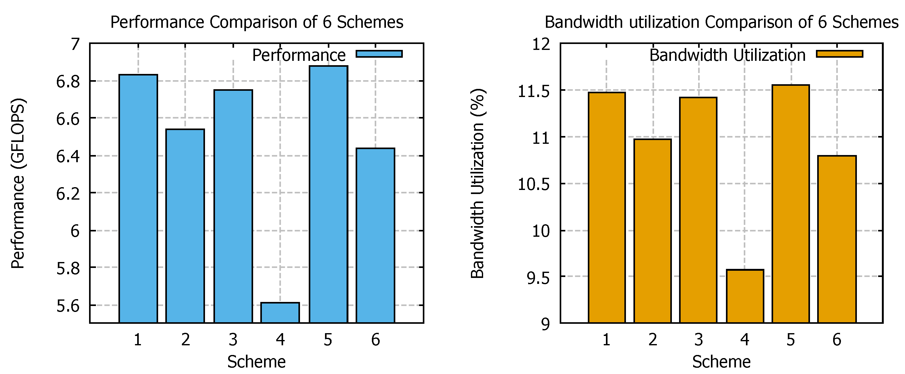
• We explore the optimal mapping method of SpMV operation in multi-DSP architecture and get the optimal scheme that has the highest performance and the best bandwidth utilization;
• According to the optimal scheme, we have run the High Performance Conjugate Gradient (HPCG) benchmark on the accelerator, and the result proves the superiority of our design.

The rest of this paper is organized as follows. Section 3 introduces the background. Then, in Section 4, we present the super gather transmission method and hardware implementation. Section 5 describes the mapping of SpMV to the M processor and the optimization scheme. Afterwards, related work is presented in Section 2. Section 6 provides the conclusions of this paper.

2. Related Work

The algorithmic implementation of SpMV usually compresses sparse matrices to save storage resources, but this leads to the acquisition of dense vectors requiring indirect memory accesses, which consumes a lot of time. Ref. [1] proposes an FPGA architecture that maximizes the vector’s re-usability by introducing a cache-like architecture in which the cache is implemented as a circular list to maintain the BRAM vector components. In Ref. [8], machine learning technology is used to select the optimal SpMV implementation scheme (short running time and low energy consumption) applied on GPU according to the characteristics of the sparse matrix, and the accuracy is nearly 90%. Ref. [14] proposed a scheme ALBUS (Absolute Load Balancing Using SIMD (Single Instruction Multiple Data)) that improves the performance of SpMV in multi-core systems by balancing load and SIMD vectorization. Ref. [15] proposed a learning-based sparse meta-format method, BestSF (Best Sparse Format), which supports automatic selection of the optimal sparse format for a given input matrix by a cost-sensitive classification system.

3. Background

3.1. The ELL Storage Format and the SpMV Algorithm

Figure 1a shows the SpMV calculation. A is the sparse matrix, x is the dense vector, and y is the product of A and x, i.e., $y=Ax$. Figure 1b shows the ELL storage format of the sparse matrix. The sparse matrix A is compressed to obtain the numerical matrix ($A\_v$) and index matrix ($A\_i$). The $A\_v$ can be generated by gathering the non-zero elements of the sparse matrix to the left in each row. The columns are the number of non-zero elements in the row that has the most non-zero elements. The empty positions in other rows are supplemented by 0 in $A\_v$. The $A\_i$ is the column number of each element of the $A\_v$ in the original matrix, A, and the column number of zero elements is arbitrary (“*” in the Figure 1b), which is generally set to 0. The $A\_v$ and $A\_i$ are continuously stored in memory by columns, which facilitates the use of vector loading instructions to load data.

Algorithm 1 shows the SpMV algorithm of the ELL storage format. $row\_width$ and $col\_width$ are the number of rows and columns of the $A\_v$, respectively. The elements of $A\_v$ in the algorithm are accessed sequentially, while the data of the dense vector x needs to be obtained according to the index corresponding to the elements of $A\_v$ by the indirect memory access, which degrades the performance of SpMV [16]. Therefore, SpMV is an algorithm with an obvious memory access bottleneck.

Algorithm 1 SpMV Algorithm of ELL Storage Format

1: for$i=0$; $i<row\_width$; $i++$do 2:     $y\left[i\right]=0$ 3:     for $j=0$; $j<col\_width$; $j++$ do 4:         $y\left[i\right]+=A\_v[i\ast row\_width+j]\ast x[A\_i[i\ast row\_width+j\left]\right]$ 5:     end for 6: end for

3.2. M Processor Architecture

The M processor is a multi-DSPs processor that includes two clusters with the same structure. Figure 2 shows the overview of the cluster (purple rectangle). It has six super-nodes (SNs) (blue rectangle), and each SN includes four DSP cores (green rectangle). The DSP core is composed of a very long instruction word (VLIW) controller, a scalar processing unit (SPU), a vector processing unit (VPU), DMA, and array memory (AM). The SPU that performs scalar calculations consists of scalar processing elements (SPE) and scalar memory (SM). VPU consists of 16 vector processing elements (VPEs), each of which has three Multiplier and Accumulation (MAC) to enable vector fixed-point and floating-point operations. Single instruction multiple data (SIMD) parallel technology executes the VLIW instruction on vector data. In addition, DSP has a DMA component inside, which can transfer data between the inside memory (i.e., SM, AM) and tge outside memory (i.e., high bandwidth memory (HBM), global shared memory (GSM)) quickly and without occupying the instruction. Transferring data between HBM and GSM is also allowed by DMA. DMA has three pillars of host physical channels, which generate the data transfer request according to program instructions. Among them, two general channels (GPip0 and GPip1) enable traditional data transfer, and the last one, APip, allows the efficient data transfer from the off-chip memory to the on-chip memory by the indirect memory accesses, which can speed up the running speed of the algorithm with the access bottleneck. We introduce the APip in detail in Section 4.2. The priority of channels from highest to lowest is APip, GPip0, and GPip1. These three channels share the data bus and occupy it according to the channel priority. The multi-level data network adopts the Advanced eXtensible Interface (AXI) network protocol. Besides, each cluster has sufficient storage resources (such as HBM, and GSM).

4. Methods and Design

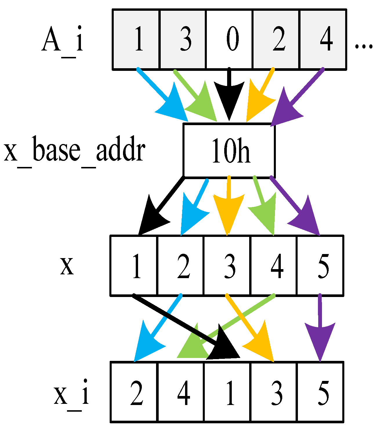
In combination with the hardware resources of the M processor and the characteristics of various sparse matrix compression formats, the ELL format is selected to compress and store the sparse matrix in this paper, which is conducive to giving full play to the parallel computing power of the processor [17,18].

4.1. SuperGather

The main reason affecting the running speed of the SpMV algorithm is that the access to specific elements in x is irregular and gives rise to a very long time-consuming process. We propose an indirect memory accesses scheme called SuperGather (SG) for DMA.

As shown in Figure 3, $A\_i$ is the index matrix obtained by compressing the sparse matrix in ELL format, x is the dense vector, and $x\_base\_addr$ is the first address of X in the main memory. We get the index from $A\_i$ and add $x\_base\_addr$ to generate the actual address of the desired x element, then fetch the corresponding x (i.e., $x\_i$) from the main memory to the DSP inner memory. The $x\_i$ is multiplied by the corresponding $A\_v$ element of $A\_i$.

4.2. A Dedicated Channel

We design a dedicated host channel in the DMA to realize the Super Gather Transfer Mode (SGTM) to speed up the process of irregular access data.

The $A\_v$ and $A\_i$ of sparse matrix and the dense vector x are all stored in the HBM. The base address and size of these matrices in HBM are known in advance. Therefore, we use the index in $A\_i$ corresponding to the numerical elements in $A\_v$ as the index of the element in x, and the address offset can be obtained by appropriately extending the index. Then, the right x element ($x\_i$) is accessed by combining the base address of x with offset and is then moved to the AM in DSP. This process is implemented in the APip channel in DMA. The main difference between the APip channel and GPip0/1 is that the configured source parameters of the APip channel generate the address to read the $A\_i$, not the source data. In addition, the $A\_i$ data should return to this channel and then be combined with the base address of the dense vector to generate the actual address of $x\_i$ to be accessed.

Figure 4 is the APip structure that uses the state machine to control the executed state, including the following five states: Idle (not shown), UpdateParm, RdIndex, RdData, and Finish.

(1) Idle: In the initial case, the state machine is at the state. When the APip channel starts, it jumps to the state of UpdateParm.

(2) UpdateParm: Get the new transmission parameters from RAMIntf and update the relevant registers in the channel. Jump to RdIndex state after parameter update is completed.

(3) RdIndex: Generate the read index address according to the source parameters, and then send the request of the read index. Each batch can issue eight index reading requests. The returned index data is stored in the FIFO at this channel while it counts to determine whether the indexes required all the returns. When the indexes are all returned, jump to RdData state. During this period, if there is an abnormal signal, the state will jump to Idle state and report an error to the system.

(4) RdData: Firstly, get the index from the index FIFO and extend it appropriately to generate the address offset, and then add to the base address to generate the actual source data address. Meanwhile, get the data write-address according to the destination parameters. Then, send the read request and wait for a response signal that implies that the data has already moved to the destination address. The response signal is counted and compared with the desired number to judge whether the batch read-data requests are processed. If the amount of data that has moved meets the data amount defined in the transmission parameters, jump to the state of Finish. If not, repeat steps (3) and (4) until all data move to the destination successfully. During this period, if there is an abnormal signal, jump to the Idle state and report an error to the system.

(5) Finish: Main completion: a. generation of transmission completion signal; b. write parameters back to RAMIntf; c. the function of parameter linking or channel linking is carried out according to the relevant bit fields in the transmission parameters.

4.3. The Algorithm Structure

To improve the performance of SpMV, we adopt the double buffering method to make the data transfer overlap with part of the computing time.

Figure 5 shows the schematic diagram of data movement and computation. After compressing the sparse matrix using the ELL format, we obtain $A\_v$ and $A\_i$ which is continuously stored in HBM according to the columns. x is the vector to be indexed. Use GPip0 (or GPip1, which has the same structure and function) to move the subblocks of $A\_v$ from HBM to AM, and use APip to move $x\_i$ to AM. AM has the lower address space AM0 and higher address space AM1. The steps are as follows:

(1) $A\_v$ subblock moves to the lower address space of AM0 and $x\_i$ moves to the higher address space of AM0. Note that, according to Algorithm 1, the amount of $A\_v$ and $x\_i$ is the same;

(2) Load the $A\_v$ and $x\_i$ in AM0 into VPU for calculation. Meanwhile, the new subblock data of $A\_v$ and $x\_i$ moves into AM1;

(3) Similar to (2), the $A\_v$ and $x\_i$ of AM1 move into VPU for calculation. Meanwhile, the new subblock data of $A\_v$ and $x\_i$ moves into AM0;

(4) Repeat (2) and (3) until all data calculations are complete.

Note that the final computing result of each block restores to AM and then transfers to HBM, which is not shown in Figure 5.

The three host physical channels (APip, GPip0, and GPip1) in DMA are in descending order of priority, and all share the same data path. While the higher priority channel occupies the data path, the lower priority channel should wait for the data channel to be free before using it. Thus, there are two SpMV algorithm schemes (i.e., schemes 1 and 2), as shown in Figure 6. The difference between the two schemes is the moment of GPip0/1 and APip. The GPip0/1 and APip serially start in scheme 1, but parallelly start in scheme 2. When the APip channel is running, a batch of reading index requests are sent first, and it then waits for all index returns to this channel before executing the subsequent functions. When APip is in the waiting period, the data path is idle and can apply to GPip0/1.

Referring to the structures of the algorithms, there are two algorithm flow charts, as shown in Figure 7. There are five main functions (the five colors in Figure 7): Initial system, DMA configuration, DMA start, DMA end check, and SpMV calculation.

5. SpMV Mapping on the M Processor

5.1. Performance Calculation Principle

Sparse matrix and dense vector data are 64-bit double-precision floating-point numbers conforming to the IEEE-754 standard. The performance of SpMV can be expressed as the ratio of the number of floating-point operations performed to the running time, in Floating-point operations (FLOPS). Equation (1) is the calculation formula of SpMV performance, in which t represents the running time of the SpMV algorithm in seconds (s), and the total floating-point operand is related to the size of the compressed sparse matrix. $A\_row$ and $A\_col$ are the numbers of rows and columns of the $A\_v$, respectively. The elements of $A\_v$ are all subject to floating-point multiplication and addition operations, so the number of floating-point operands is twice the number of that in $A\_v$.

$$SpMV\_performance=\frac{A\_row\times A\_col\times 2}{t}$$

(1)

5.2. Optimization of the SpMV Algorithm

Experiment Setup. We implemented the Register Transfer Level (RTL) of this design in Verilog and carried out clock-accurate simulation. We set the DSP frequency to 1.8 GHz, the data network working frequency to 1.2 GHz, and the HBM working frequency to 600 MHz. All DSP cores of the two clusters work at the same time, and each core has the same workload. The size of the $A\_v$ and $A\_i$ obtained by ELL format compression is $1152\times 512\times 2$, and the number of x vector elements is $192\times 128\times 128\times 2$.

There are three host physical channels in the DMA of each DSP core, which can make up many data transfer schemes. The bandwidth utilization in each scheme is different, and the SpMV performance will also be inconsistent. The algorithm structure of scheme 1 and scheme 2 in Section 4.3 (see Figure 6) shows the performance of 48 cores measured as shown in Figure 8. The SpMV performance of scheme 1 is higher than that of scheme 2, reaching 6.83 GFLOPS, and the bandwidth utilization is 11.48%. So, with two host physical channels, the DMA channel GPip0/1 and APip, a serial start has higher performance than the parallel start way. Due to the sparse data and x being in HBM, request from the two channels of the data transfer path has much overlap. If it starts two channels at the same time, the requests in the network will become complex and decrease transfer efficiency. In addition, the low bandwidth utilization indicates that the performance of SpMV is mainly affected by the large amount of time consumed in the access process. GPip0/1 can make full use of the bandwidth to transfer the elements in the $A\_v$ and $A\_i$, while the APip channel with SGTM only uses about 1/8 of the bandwidth for the removal of x, which accounts for the major part of the access time.

SpMV algorithm optimization. By analyzing the working state of the processor on schemes 1 and 2, we have found that when multicore programs run the SpMV algorithm at the same time, it produces many requests to access HBM (including reading $A\_i$, $A\_v$, x). The data network can experience severe congestion, and the HBM is accessed slowly, thereby increasing the DMA data transfer time.

GSM has a faster access speed than HBM, so it is well worth a try to move some data from HBM to GSM in advance to relieve the access pressure of HBM. Combined with the storage capacity of GSM and algorithm structure, We have come up with a new scheme: use GPip0/1 to move the subblock of $A\_i$ from HBM to GSM, and then the rest steps of the algorithm are performed. So, schemes 3 and 4 are obtained based on algorithm schemes 1 and 2, as shown in Figure 6.

As shown in Figure 8, the order of computational performance (and bandwidth utilization) from high to low are 1, 3, 2, and 4. Compared with 1 and 3 (or 2 and 4), the direct way that uses GPip0/1 to move $A\_i$ from HBM to GSM and then uses the APip channel to get $x\_i$ is worse than the straightforward way that uses APip channel directly to get $x\_i$ from HBM. Surprisingly, the performance and bandwidth utilization of scheme 4 are significantly lower than that of scheme 2. It does not highlight the advantage of GSM’s fast access speed and the effect of alleviating the pressure of HBM access.

The program executed by each DSP core is the same, and the load is also equal. The process that moves the index from HBM to GSM in schemes 3 and 4 runs in each DSP core, and there is a large number of request blocking phenomena, which affects the efficiency of data moving. Therefore, to obtain the best migration effect, it is necessary to find out the optimal number of DSP cores used in the migration index data and the location of each DSP core.

We measured the moving time using different cores in one cluster, as shown in Figure 9. We find that using four DSP cores, each of which is in a different supernode, uses the shortest time. After modifying scheme 3 and scheme 4, we get scheme 5 and scheme 6 in Figure 6.

Figure 8 shows the performance and bandwidth utilization comparison of all six schemes. The computational performance and data bus bandwidth utilization of SpMV in schemes 5 and 6 are improved compared to schemes 3 and 4,which is in line with our expectations. Moreover, the behavior of scheme 5 is the best among all the schemes, reaching 6.88 GFLOPS and 11.56% bandwidth utilization. Although scheme 6 improved the performance and bandwidth utilization very much on the base of scheme 4, it is not as good as scheme 2. This is because the time cost of transferring A_i from HBM to GSM is larger than that of the frequent computation of bandwidth of the two parallel that started the channel in the data path.

HPCG performance. We use the HPCG benchmark program to evaluate the performance of the supercomputer systems. SpMV is one of the essential algorithms in HPCG and is critical to its behavior. We run the HPCG program on an M processor and get an average performance of 2.8 GFLOPS.

6. Conclusions

The SpMV algorithm is widely used to solve practical problems, but it has an obvious bottleneck of access to storage. Improving its access efficiency will enhance the computing performance. The M processor has multiple DSP cores (i.e., abundant parallel computing resources) and plentiful storage resources. We propose a kind of data transmission method named SuperGather and design a dedicated host physical channel APip in the DMA of DSP, which can implement the indirect memory accesses to accelerate the SpMV calculation. Combined with hardware structure and process analysis, we propose six algorithm schemes and then analyze the characteristics of these schemes in detail. Finally, we find the best algorithm scheme (scheme 5) with the best performance and bandwidth utilization, which makes the SpMV algorithm achieve higher performance on M processor, up to 6.88 GFLOPS. We also run the HPCG benchmark, and the average performance is 2.8 GFLOPS. In the future, we will optimize our design and compare our design with more state-of-the-art designs.

References

1. Oyarzun, G.; Peyrolon, D.; Alvarez, C.; Martorell, X. An FPGA cached sparse matrix vector product (SpMV) for unstructured computational fluid dynamics simulations. arXiv 2021, arXiv:2107.12371. [Google Scholar]
2. Demirci, G.V.; Ferhatosmanoglu, H. Partitioning Sparse Deep Neural Networks for Scalable Training and Inference. In Proceedings of the ACM International Conference on Supercomputing, Virtual, 14–17 June 2021; Association for Computing Machinery: New York, NY, USA, 2021; pp. 254–265. [Google Scholar] [CrossRef]
3. Langr, D.; Tvrdík, P. Evaluation Criteria for Sparse Matrix Storage Formats. IEEE Trans. Parallel Distrib. Syst. 2016, 27, 428–440. [Google Scholar] [CrossRef]
4. Bell, N.; Garland, M. Implementing sparse matrix-vector multiplication on throughput-oriented processors. In Proceedings of the Conference on High Performance Computing Networking, Storage and Analysis, Portland, OR, USA, 14–20 November 2009; pp. 1–11. [Google Scholar] [CrossRef] [Green Version]
5. Kourtis, K.; Karakasis, V.; Goumas, G.; Koziris, N. CSX: An Extended Compression Format for SpMV on Shared Memory Systems. In Proceedings of the 16th ACM SIGPLAN Symposium on Principles and Practice of Parallel Programming, PPOPP 2011, San Antonio, TX, USA, 12–16 February 2011; Volume 46, pp. 247–256. [Google Scholar] [CrossRef]
6. Liu, W.; Vinter, B. CSR5: An Efficient Storage Format for Cross-Platform Sparse Matrix-Vector Multiplication. In Proceedings of the 29th ACM on International Conference on Supercomputing, Newport Beach, CA, USA, 8–11 June 2015. [Google Scholar] [CrossRef]
7. Yan, S.; Li, C.; Zhang, Y.; Zhou, H. yaSpMV: Yet another SpMV framework on GPUs. In Proceedings of the 19th ACM SIGPLAN Symposium on Principles and Practice of Parallel Programming, Orlando, FL, USA, 15–19 February 2014; Volume 49, pp. 107–118. [Google Scholar] [CrossRef]
8. Dufrechou, E.; Ezzatti, P.; Quintana-Ortí, E. Selecting optimal SpMV realizations for GPUs via machine learning. Int. J. High Perform. Comput. Appl. 2021, 35, 254–267. [Google Scholar] [CrossRef]
9. Katagiri, T.; Sato, M. An Auto-tuning Method for Run-time Data Transformation for Sparse Matrix-Vector Multiplication. IPSJ SIG Notes 2011, 41, 130. [Google Scholar]
10. Guo, P.; Wang, L.; Chen, P. A Performance Modeling and Optimization Analysis Tool for Sparse Matrix-Vector Multiplication on GPUs. IEEE Trans. Parallel Distrib. Syst. 2014, 25, 1112–1123. [Google Scholar] [CrossRef]
11. Li, J.; Tan, G.; Chen, M.; Sun, N. SMAT: An Input Adaptive Auto-Tuner for Sparse Matrix-Vector Multiplication. In Proceedings of the 34th ACM SIGPLAN Conference on Programming Language Design and Implementation, Seattle, WA, USA, 16–19 June 2013; Association for Computing Machinery: New York, NY, USA, 2013; pp. 117–126. [Google Scholar] [CrossRef]
12. Sedaghati, N.; Mu, T.; Pouchet, L.N.; Parthasarathy, S.; Sadayappan, P. Automatic Selection of Sparse Matrix Representation on GPUs. In Proceedings of the 29th ACM on International Conference on Supercomputing, Newport Beach, CA, USA, 8–11 June 2015; Association for Computing Machinery: New York, NY, USA, 2015; pp. 99–108. [Google Scholar] [CrossRef]
13. Neelima, B.; Reddy, G.; Raghavendra, P. A GPU Framework for Sparse Matrix Vector Multiplication. In Proceedings of the 2014 IEEE 13th International Symposium on Parallel and Distributed Computing, Marseille, France, 24–27 June 2014; pp. 51–58. [Google Scholar] [CrossRef]
14. Bian, H.; Huang, J.; Liu, L.; Huang, D.; Wang, X. ALBUS: A method for efficiently processing SpMV using SIMD and Load balancing. Future Gener. Comput. Syst. 2021, 116, 371–392. [Google Scholar] [CrossRef]
15. Benatia, A.; Ji, W.; Wang, Y.; Shi, F. BestSF: A Sparse Meta-Format for Optimizing SpMV on GPU. ACM Trans. Archit. Code Optim. 2018, 15, 1–27. [Google Scholar] [CrossRef] [Green Version]
16. Vuduc, R.W.; Moon, H.J. Fast Sparse Matrix-Vector Multiplication by Exploiting Variable Block Structure. In Proceedings of the High Performance Computing and Communications, Austin, TX, USA, 15–20 November 2015; Yang, L.T., Rana, O.F., Di Martino, B., Dongarra, J., Eds.; Springer: Berlin/Heidelberg, Germany, 2005; pp. 807–816. [Google Scholar]
17. Monakov, A.; Lokhmotov, A.; Avetisyan, A. Automatically Tuning Sparse Matrix-Vector Multiplication for GPU Architectures. In Proceedings of the High Performance Embedded Architectures and Compilers, Pisa, Italy, 25–27 January 2010; Patt, Y.N., Foglia, P., Duesterwald, E., Faraboschi, P., Martorell, X., Eds.; Springer: Berlin/Heidelberg, Germany, 2010; pp. 111–125. [Google Scholar]
18. Liu, X.; Smelyanskiy, M.; Chow, E.; Dubey, P. Efficient Sparse Matrix-Vector Multiplication on X86-Based Many-Core Processors. In Proceedings of the 27th International ACM Conference on International Conference on Supercomputing, Eugene, OR, USA, 10–14 June 2013; Association for Computing Machinery: New York, NY, USA, 2013; pp. 273–282. [Google Scholar] [CrossRef]
Figure 1. SpMV calculation and ELL storage format.
Electronics 11 03699 g001
Figure 2. Cluster overview.
Electronics 11 03699 g002
Figure 3. SuperGather.
Electronics 11 03699 g003
Figure 4. APip structure.
Electronics 11 03699 g004
Figure 5. Data movement and calculation.
Electronics 11 03699 g005
Figure 6. Six algorithm structures. We introduce the first two schemes (1 and 2) in Section 4.3 and the other four schemes in Section 5.2. We have the following definition in this figure: A: the sparse matrix data; A _ i : the sparse matrix index data; x: the x data; h: HBM; gg: GSM; a 0 : the lower half address storage space of AM; a 1 : the higher half address storage space AM; A h a 00 : the A is moved from HBM to AM00 in the low land address space of AM0. A _ i h g : transfer A_i from HBM to GSM; x g h a 01 : get A_i from GSM, and then transfer indexed x data from HBM to AM01; c o m p u t e : the calculation of the data. The other markers are similar.
Electronics 11 03699 g006
Figure 7. Flowchart for the two algorithms.
Electronics 11 03699 g007
Figure 8. Six scheme performance and bandwidth utilization comparison.
Electronics 11 03699 g008
Figure 9. Time comparison of different moving modes. The “SN00” represents the core 0 of the supernode 0 (SN0), and “SN0” represents the four cores in the supernode. The other markers are similar.
Electronics 11 03699 g009
Publisher’s Note: MDPI stays neutral with regard to jurisdictional claims in published maps and institutional affiliations.