Anomalous Behavior Detection Based on the Isolation Forest Model with Multiple Perspective Business Processes

Abstract

Anomalous behavior detection in business processes inspects abnormal situations, such as errors and missing values in system execution records, to facilitate safe system operation. Since anomaly information hinders the insightful investigation of event logs, many approaches have contributed to anomaly detection in either the business process domain or the data mining domain. However, most of them ignore the impact brought by the interaction between activities and their related attributes. Based on this, a method is constructed to integrate the consistency degree of multi-perspective log features and use it in an isolation forest model for anomaly detection. First, a reference model is captured from the event logs using process discovery. After that, the similarity between behaviors is analyzed based on the neighborhood distance between the logs and the reference model, and the data flow similarity is measured based on the matching relationship of the process activity attributes. Then, the integration consistency measure is constructed. Based on this, the composite log feature vectors are produced by combining the activity sequences and attribute sequences in the event logs and are fed to the isolation forest model for training. Subsequently, anomaly scores are calculated and anomalous behavior is determined based on different threshold-setting strategies. Finally, the proposed algorithm is implemented using the Scikit-learn framework and evaluated in real logs regarding anomalous behavior recognition rate and model quality improvement. The experimental results show that the algorithm can detect abnormal behaviors in event logs and improve the model quality.

1. Introduction

Business process management analyzes system execution records to detect and optimize information systems. In the era of Big Data, information systems generate many execution records, bringing a wealth of data for business process management. However, these data are not entirely usable and are mixed with behaviors that deviate from those defined by business processes. They occur infrequently but can jeopardize system security and hinder the progress of analysis, such as fraud detection, data leakage, and intrusion detection. Therefore, how to detect and remove these deviations is of vast concern to enterprises. The anomalous behavior is related to the sequence of process activities, the relationship between activities, or attribute non-compliance, therefore the anomaly detection (outlier detection) techniques in the field of data mining are struggling to be applied to business processes. Anomalous behavior detection is a popular automated business process management technique that ensures data availability by identifying deviations from standard specifications by learning process rules based on the behavior that has occurred and serves as an essential task in business process management [1].

There are three types of anomalous behaviors in practical scenarios which are as follows: (1) anomalous behaviors caused by events that deviate from the normal situation at the control flow level; (2) anomalous behaviors caused by control flow levels that are legal, such as legal in process structure and sequence but not legal in data attributes; and (3) anomalous behaviors caused by events with legal data attributes (e.g., conforming to the value range of data) but illegal in their associated process structure. Current anomalous behavior detection algorithms mainly determine whether the activities in the event log conform to expectations from the control flow perspective. Conformance-checking techniques are a common approach to detecting deviations from expectations by aligning the event log and the reference model [2]. In addition, there are many anomaly detection methods based on numerical fluctuation patterns, such as relative density-based anomaly detection [3], clustering-based anomaly detection [4], and distance (or density)-based anomaly detection [5]. These algorithms ignore the impact of data attributes or activity relationships in event logs on anomalous behavior detection.

To address this, an isolated forest model based on fused consistency features and an anomalous behavior detection method is constructed. The isolated forest model is constructed by analyzing activity–behavior and attribute-matching relationships from control and data flow perspectives. Then, the integration consistency measure is proposed by analyzing the multi-view log feature. The composite log feature vector is constructed by mining historical information to achieve business process anomalous behavior detection based on different threshold-setting strategies. The research method in this paper consists of three main steps (Figure 1).

(1) Based on the control flow perspective, the K-order neighborhood behavioral relationships between the model and the log activities are analyzed. The activities occurring in the traces are mapped to the corresponding ones in the model. The joint neighborhood of each activity is found based on the behavioral relationship between the activities. The neighborhood consistency value of the activity is then calculated using the neighborhood distance. Further, the behavioral consistency degree of the current trace and the model is calculated.

(2) Calculate the attribute distance by classification alignment based on the data flow perspective. The attribute information corresponding to each event is extracted from the model based on the control flow constraint. Based on the trace and the execution trace where the activities in the model are located, the data attribute information of each event is matched one by one based on the idea of alignment. Then, the cost of mismatch between the trace and the model based on the data attributes is calculated based on the standard cost function of alignment. After obtaining the mismatch cost and normalizing it, the attributes’ degree of consistency in the trace and the model based on the data flow perspective can be calculated.

(3) Construct a composite trace vector and use an isolation forest model for anomalous behavior detection based on different threshold strategies. The degree of behavioral consistency from the control flow perspective and the degree of attribute consistency from the data flow perspective are considered together to obtain the degree of trace- and model-based integrated consistency. Next, a composite feature vector is constructed based on the logs’ integrated consistency degree and other information. Three different setting strategies select the threshold and the proposed vector is used as input data to train the isolation forest model and perform anomalous behavior detection.

2. Problem Statement

A Petri net structure of the insurance claims process (Figure 2) depicts some of the activities in the insurance claims process. The circle represents a place. The rectangle represents a transition and the words in a rectangle indicate an activity performed in the current event. A dashed line connects each variation to a dashed box, describing the data attributes carried by executing the current event.

While there is various data attribute information of events in real life, only four types of attribute information are shown in the Petri diagram of this paper: User, Resource, Timestamp, and Duration. In this example, the User is divided into three roles: client, staff, and manager. The Resource is the material the User requires to execute the current event. The Timestamp refers to the days in a week when the current event can be performed. The Duration refers to the time of day when the current event can be executed. For example, the first transition customer report in the diagram indicates the execution of a customer report activity. The event is performed by the client, requires the submission of relevant certifications, and can be reported anytime from Monday to Sunday. Similarly, a case handling indicates that a case handling activity is performed, which is executed by the client’s manager, who has to negotiate with the client on the claim amount, and the manager only handles the case between 8:00 and 17:00 on Friday.

The Petri net shows that each event’s data attribute is critical to the current execution activity and the relationship between the data attribute and the execution activity cannot be ignored.

Table 1. Event log fragments.

Event Id	Case Id	Activity	User	Resource	Timestamp
…	…	…	…	…	…
671	476	a	client	certifications	Monday
672	476	b	staff	archive	Monday
673	477	h	manager	\	Thursday
674	476	c	staff	loggers	Tuesday
675	477	e	staff	check	Wednesday
676	478	a	client	certifications	Monday
677	476	e	staff	check	Wednesday
678	476	f	staff	quoted price	Thursday
679	478	b	staff	archive	Tuesday
680	476	g	manager	staff	Friday
681	477	d	staff	evaluation	Tuesday
…	…	…	…	…	…

gives a fragment of the event log in the system, where three facts, User, Resource, and Timestamp, are considered. For example, if we look at event 673, it corresponds to the activity failed present in the model. There is no exception if we consider only the control flow. However, when looking at its dataflow properties, we can see that it occurs on Thursday (“Thursday”), which does not match the timestamp property Friday (“Friday”), where the activity “failed” appears in the model. Similarly, the activity "case handling" corresponding to the event 680 is consistent with the model. However, when considering its resource attribute ("staff"), it is not consistent with its counterpart ("client") in the model. Therefore, the activities executed in events 673 and 680 are consistent with the expected behavior. However, they are anomalous because the Timestamp or Resource attributes in the events are incompatible with the data attributes of the corresponding events executed in the model. In summary, both activities and attributes can lead to anomalous situations. Therefore, Anomalous Behavior Detection should focus on the activities for each event in the control flow perspective and consider the attribute information in the data flow perspective.

3. Related Works

Diverse system runtimes, such as system failures or suboptimal resource behavior, can cause the event log to be error-prone. Errors in event logs hinder the extraction of helpful process details from event log analysis. Consequently, many scholars have focused on detecting anomalies in event logs. To address the problem that consistent alignment techniques prioritize the control flow perspective and ignore data attribute constraints, a deviation detection algorithm based on a customizable cost function is proposed [6]. Fani Sani et al. propose a data preprocessing method for detecting and repairing anomalous behavior that uses activity occurrence probabilities and behavioral context information to identify and repair anomalies and experimentally verify that the proposed method can provide more reliable input to existing process mining algorithms [7]. To address the problem of anomaly detection in business processes, an autoencoder-based anomaly detection method DAE was proposed, which can analyze the causes of business process anomalies in events at a fine-grained level and can detect information such as the type of anomaly and the time of occurrence [8]. Bezerra et al. analyzed three anomaly detection algorithms, threshold, iterative, and sampling, and used accurate event logs to evaluate the three methods and arrive at the best detection algorithm [9]. The threshold algorithm considers event traces below a threshold value as anomalous; the iterative algorithm considers minimal consistency as anomalous; and the sampling algorithm considers activities that are not present with the sample model as anomalous. These three methods ignore the effect of data attributes from the control flow perspective.

Process anomaly detection methods focus only on individual deviating activities, ignoring the correlation between anomalous behaviors and the impact of parallel relationships. An anomaly frequent pattern extraction method is proposed to solve this problem, which applies to anomaly detection of parallel activities [10]. Van Zelst et al. proposed a prefix-aligned online consistency detection method. To solve the shortest path-solving problem, two path-solving methods based on optimal efficiency and memory performance balancing were designed to improve the consistency detection efficiency significantly [11]. A frequent pattern-based anomaly detection method is proposed to detect behavioral deviations in event logs and process models. The method mines the expected behaviors in the process and constructs partial models by clustering and frequent pattern approaches to detect the anomalies present in the model and event log [12]. A clustering-based anomaly detection method is proposed for the problems of memory and domain knowledge limitations online, which uses a recursive approach to detect anomalous behaviors in traces [13]. Supervised and semi-supervised scenarios are considered, and online learning techniques are combined to achieve early detection of anomalies, which significantly improves the efficiency of anomaly detection [14]. A combined online learning technique and trace anomaly detection method is proposed to achieve real-time monitoring of incomplete traces, calibrating anomaly thresholds by multiple parameters to meet the online anomaly detection needs in different scenarios [15].

Because of the limited control flow knowledge, some studies have focused on additional constraints from the data flow level. A chronological anomaly detection method is proposed to address the problem similar to fraudulent combination attacks. Execution time anomalies are detected in multiple directions by detecting the differences in temporal behavior between historical traces and traces being executed, taking into account the temporal dependencies between the current event and the preceding and following activities [16]. A DBPMN model was designed based on BPMN and DMN (decision table) to interact with processes and decisions, which combines behavioral decision-making with data perception and paves the way for studying behavior and attribute dependencies [17]. Tavares et al. implemented real-time monitoring of business processes using online event stream input, dynamically extracting relevant information from event logs. Based on clustering methods, real-time detection of anomalous behavior in business processes enables the processing of dynamic data [18]. Ebrahim et al. proposed an unsupervised anomaly detection method based on an organizational perspective and control flow perspective, which differs from traditional anomaly detection methods by not treating low-frequency events as anomalies but detecting illegal user executions and events not executed according to the regular model [19].

However, existing studies have limited utilization of inter-activity dependencies or data-level constraints, therefore, in this paper, we take the activity information of control flow as the main body and fuse the attribute alignment relationships at the data flow level for analysis, to achieve isolated forest model construction and anomalous behavior detection under multi-perspective constraints.

4. Preliminary

This section introduces the basics used in this paper, including the concepts of event logs, traces, log-based sequential relationships, Petri net, and its weak behavioral relationships. In addition, we briefly introduce the common terminology and steps for anomaly detection based on the isolation forest model.

4.1. Behavioral Relationships in Event Logs

Often, information systems record in great detail what specific activities were performed by a running instance of a process (also called a case) at a point in time. Process mining techniques aim at analyzing such data, i.e., event logs, mainly in a static/posterior setting, i.e., only for completed cases. In Table 1, each row indicates that an event was executed in the context of an insurance claim process, identified by the event id (Event-id); similarly, this instance is recorded by the case id (Case-id). An event contains several data attributes, such as Event-id, Case-id, the activity executed, the User, the Resources used by the User, and the Timestamp.

Observe the events associated with the case id 476. The first event, with an event id of 671, describes that the client (client) performed the activity reported by the client. Subsequently, the case is accepted by the staff (Staff) (Event-id 672). Next, the staff conducts a public assessment of the case (Event-id 674), checks the details of the case (Event-id 677), and performs a verification of the loss (Event-id 678). Finally, the manager registers a case and communicates with the customer about the payment measures (Event-id 680). In Table 1, it can be seen that event 673 is executed between events 672 and 674, which is related to case id 477, thus indicating that several process instances can run in parallel.

In addition to the behavioral relationships between the executed activities in the control flow, we need to introduce information about the attributes contained in each event. We use the capital letter E for the complete set of events, C for the full set of case identifiers, A for the complete set of activities, U for the set of users, and R for the set of resources used by users in performing activities, and T for the set of timestamps. Two projection functions are assumed to represent the case identifier and the executed activity in the event, namely ${\pi }_C:E\to C$, and ${\pi }_A:E\to A$, respectively. The concept of event log and trace is formally identified in Definition 1.

Definition 1 (event, event log, trace) [20].

Let character E denote the set of events, character A represents the set of activities, and character C means the set of case identifiers. An event $e\in E$describes an activity executed in the context of some process instance. The trace t associated with the case $c\in C$is a sequence $\sigma \in E^{*}$, for which:

(1) $\forall 1\le i\le \left|\sigma \right|,{\pi }_C(\sigma (i))=c$, indicating that the events $\delta$ are associated with the case $c$;

(2) $\forall e\in E,{\pi }_C(e)=c\Rightarrow \exists 1\le i\le \left|\sigma \right|(\sigma (i)=e)$, indicating that every event associated with $c$ is in $\sigma$;

(3) $\forall 1\le i\le j\le \left|\sigma \right|,\sigma (i)\ne \sigma (j)$, all events in $\delta$ are unique;

(4) Use the symbol $fr{e}_a(\sigma )$ to denote the frequency of occurrence of the activity $a\in A$ in the trace $\sigma$.

In the following, the definition of sequential relations in the event log is given according to Definition 1.

Definition 2 (log-based sequential relation,${\succ }_L$) [21].

Given a set of events$e\in E$, there is a partial order relationship between the events in the event log L., i.e.,${\succ }_L=(e,\succ )$. For$\forall 1\le i\le j\le \left|\sigma \right|(\sigma (j)\cancel{\succ }\sigma (i))$, it is shown that all the events in$\sigma$need to obey their order and$a,b\in A,a{\succ }_{L}b$when$\exists \sigma =a_1{a}_2\mathrm{\dots }{a}_n,i\in \left\{1,2,\mathrm{\dots },n-1\right\}:\sigma \in L\wedge a_i=a\wedge a_{i+1}=b$.

Next, the definition of Petri nets in the process model and their behavioral weak order relations are presented.

Definition 3 (Process model Petri net) [22].

The process model Petri net$PN=(P,T,F,C)$is a quaternion that satisfies the following conditions:

(1) P is a finite set of places and T is a finite set of transitions;

(2) $P\ne \phi ,T\ne \phi$ and $P\cap T=\phi$;

(3) $F=(P\times T)\cup (T\times P)$) denotes the flow relation of PN and $(P\cup T,F)$ is a strongly connected graph;

(4) $dom(F)\cup cod(F)=P\cup T,$ where: $dom(F)=\{x\in P\cup T|\exists y\in P\cup T,(x,y\in F)\}$, and $cod(F)=\{x\in P\cup T|\exists y\in P\cup T,(y,x)\in F\}$;

(5) $C=\{and,xor,or\}$ is the structure type of the process net.

There is a weak sequential relation in the process model Petri net PN that contains $T\times T$ all the variation pairs $(x,y)$ if there exists a sequence of occurrences $\delta =t_1{t}_2\cdots t_n,$ when $i\in \left\{1,2,\mathrm{\dots },n-1\right\}$, $i<j\le n$ has $t_i=x$, and $t_j=y,x\succ y$. The definition of behavioral weak order relations is given below.

Definition 4 (Behavioral weak order relation,$\succ$) [23].

Let$(N,M_0)$be a net system on a variation set $T$, where$N=(P,T,F)$and the weak order relation$\succ \subseteq T\times T$contains all variation pairs$(x,y)$. If there exists a sequence of occurrences$\sigma =t_1{t}_2\cdots t_n$, when$(N,[i])[\sigma >,j\in \{1,\mathrm{\dots },n-1\},j<k\le n$, and then let$t_j=x,t_k=y$.

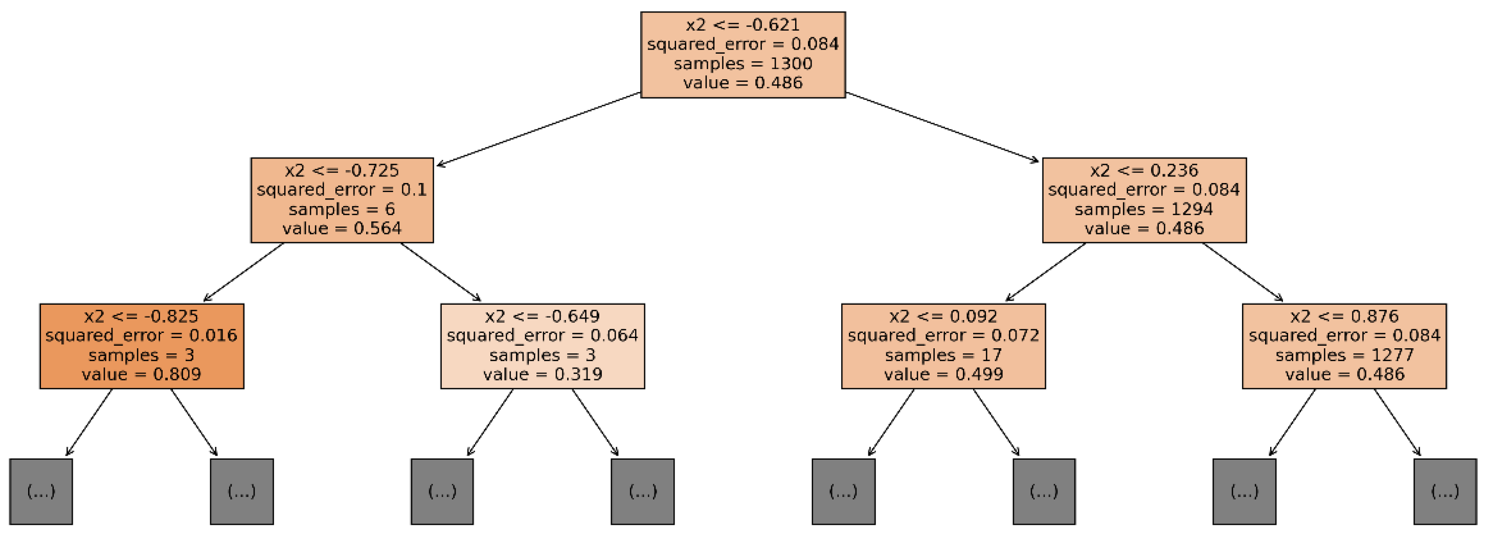
4.2. Anomaly Detection Based on the Isolation Forest Model

Isolation forest [24] is a method based on decision tree integration (ensemble). Since its introduction, it has been highly favored in industry and academia for its excellent accuracy and linear time complexity, and it plays a vital role in anomaly detection.

The core idea of isolation forest is that anomalous behavior is significantly different from other data points in some characteristics. In this setting, the anomalous samples can be quickly filtered out from the selection set by different subtrees (i.e., binary search tree structure). As shown in Figure 3, x₁ can be divided into a separate space with only one operation. In contrast, x₂ goes through seven times before it is divided into a separate space. Therefore x₁ is more likely to be anomalous behavior than x₂. If the majority of subtrees in the isolation forest agree that the sample is an outlier, the decision has high confidence.

Precisely, anomaly detection using isolation forests consists of two main steps: constructing the isolation forest structure and scoring the samples. In the first step, we need to train t subtrees iTree from the samples to build the isolation forest model. First, n samples are randomly selected from the sample set and placed in the tree’s root node. Then, the current data are segmented based on some feature (chosen randomly). Using this splitting point as the boundary, samples less than and greater than or equal to this value are placed on both sides as their left and right child nodes, respectively. The cyclic segmentation process produces t isolation trees until a limited number of times is reached or the child nodes cannot continue the segmentation.

In the second step, each sample is substituted in each iTree, and whether the data are anomalous can be determined based on the average height and the set threshold. In addition, anomaly scores can be obtained.

Definition 5 (anomaly score) [25].

$$s(x,n)=2^{-\frac{E(h(x))}{c(n)}}$$

where E(h(x)) is denoted as:

$$E(h(x))=\frac{{\displaystyle {\sum }_{i=1}^t{h}_i(x)}}{t}$$

c(n) is the average path length of an unsuccessful search in a binary search tree, denoted as$c(n)=2H(n-1)-(2(n-1)/n)$and H(i) is the summation number, which can be expressed as$H(i)=ln(i)+\gamma$, and$\gamma$ is Euler’s constant. The value domain of the anomaly score is [0,1]. When the value is close to 1, x is considered an anomaly. If the value is close to 0, it is considered normal data.

5. Multi-View Process Similarity Metric

This section presents the consistency checking metrics based on the control flow behavioral perspective and the data flow attribute perspective. First, the behavioral relationship between the event log and each activity in the model is investigated based on the control flow perspective. The related activities are identified from the model based on the activities occurring in the log trace, and then the joint neighborhood of the activities occurring in each event and the related activities in the model are obtained. Next, the neighborhood distance of the activities in each event is calculated from the common neighborhood of the log trace and the model and the common neighborhood distance of the current trace and the model can be obtained by summing them. The summed neighborhood values of the same activities in the log trace and the model are recorded as the Behavioral Consistency Degree (BCD) in the current trace and the model based on the control flow perspective.

Second, the attribute relationships between the event log and the same event data in the model are investigated based on the data flow perspective. We extract the attribute information of each event from the model and study the attribute relationship between the individual event data in the model. Then, the data attributes corresponding to each activity are extracted from the log traces. The same activities in the trace and the model were obtained in calculating behavioral consistency. The attribute information of the same activities in the trace and the model are matched separately using the idea of alignment. In turn, the cost of inconsistency between the trace and the model based on data attribute information can be calculated based on the cost function of alignment. After obtaining the cost of inconsistent data attributes in the log trace and the model, the value of the alignment of the trace with the data attribute information in the model can be calculated by normalizing it. Based on the data flow perspective, this value is noted as the Attribute Consistency Degree (ACD) of the current trace with the model.

In the following, we describe the consistency checking methods used in this section in detail. Section 5.1 focuses on the behavioral consistency measure based on the control flow perspective. Section 5.2 describes the attribute consistency measure based on the data flow perspective.

5.1. Behavioral Similarity Analysis Based on K-order Neighborhoods

In this subsection, based on the model’s event log and the control flow perspective, the behavioral relationships between the traces and the activities in the model are investigated, and their behavioral consistency degrees are calculated based on the neighborhood contexts of the activities. Firstly, the definition of a K-order neighborhood is given.

Definition 6 (K-order neighborhood).

If activity$b$is a neighborhood of activity$a$when and only when the shortest path length from activity$b$to activity$a$is$k$, denoted as$shortpathlength(a,b)=k$. Then, in the event log, the set of neighbors of order K ($k\ge 1$) of activity$a_L$is:$a_L^k=\{b_L:shortpathlength=k\}$.

The sequence of activities occurring in the trace can be obtained by considering only the control pop behavior according to the log of events occurring. We find the K-order neighbors of each activity separately according to the sequence of subsequent occurrences of each activity in the trace. Similarly, the activity sequences in the trace are then projected into the model, and the set of K-order neighborhoods in the model based on the trigger rules of the activities in the model can be obtained. Finally, based on the set of activity neighborhoods obtained in the trace and the model, we found the K-order joint neighborhood of each occurring activity in the trace and the model, which is denoted as $C_k$.

According to the trigger rules, the activities’ trigger sequence in the Petri net model can be derived according to Figure 2, as shown in Figure 4a. We take the event trace with case id 476 as an example and, based on the activities executed in the event trace, we can obtain the sequence of activities occurring in the trace, as shown in Figure 4b.

Next, the K-order neighborhood of each activity is found according to the activities’ fire order in the trace. For example, if activity a in the event trace is the initial point, its first-order neighborhood is: (a, b); the second-order neighborhood is: (a, c); the third-order neighborhood is: (a, e); the fourth-order neighborhood is: (a, f); and the fifth-order neighborhood is: (a, g). Therefore, there is an entire fifth-order neighborhood in the event trace with activity a as the initial point, as follows:

$$a_L^5=\{\stackrel{1st}{(a,b)},\underset{2nd}{(a,c)},\stackrel{3rd}{(a,e)}\underset{4th}{,(a,f)}\stackrel{5th}{,(a,g)}\}$$

Similarly, based on the trigger sequence of each activity in the model, the kth-order neighborhood of each activity in the model can be found. For example, if activity a is the initial point in the model, its first-order neighborhood is: (a, b); the second-order neighborhood is: (a, c), (a, d); the third-order neighborhood is: (a, e); the fourth-order neighborhood is: (a, f); the fifth-order neighborhood is: (a, g), (a, h); and the sixth-order neighborhood is: (a, i). Therefore, with activity a as the initial point, there are six order neighborhoods as follows:

$$a_M^6=\{\stackrel{1st}{(a,b)},\underset{2nd}{\underbrace{(a,c),(a,d)}},\stackrel{3rd}{(a,e)}\underset{4th}{,(a,f)},\stackrel{5th}{\overbrace{(a,g),(a,h)}},\underset{6th}{(a,i)}\}$$

Next, the sequence of activities in the event trace is projected into the model to find the joint neighborhood of order K for each occurring activity in the trace and the model. We take the same activity a in the trace and the model as the initial point, as shown in Figure 4, using the red dashed box shows the joint neighborhood of the trace and the model with activity a as the initial point. Its first-order joint neighborhood is (a, b); the second-order joint neighborhood is (a, c); the third-order joint neighborhood is (a, e); the fourth-order neighborhood is (a, f); and the fifth-order joint neighborhood is (a, g). Therefore, the joint neighborhood with activity a as the initial point in the trace and model has five orders, as follows:

$$C_5^{}=\{\stackrel{1st}{(a,b)},\underset{2nd}{(a,c)},\stackrel{3rd}{(a,e)}\underset{4th}{,(a,f)}\stackrel{5th}{,(a,g)}\}$$

Here, only the joint neighborhood of order K with activity a as the starting point is calculated, and so on. After projecting each occurring activity in the trace to the model, the joint neighborhood of order K for the same occurring activity in the trace and the model can be calculated.

To obtain the behavioral consistency between the trace and the model, we need to calculate the matching degree between the trace and the active neighborhood context in the model. Firstly, we need to calculate the model’s K-order neighborhood distance between the trace and the corresponding activity. Secondly, we can obtain the matching value of the current neighborhood by multiplying the K-order neighborhood distance value by the corresponding neighborhood weight value; finally, we can sum up all the neighborhoods to obtain the consistency of the current behavior between the trace and the model.

In this section, we use the vector space model (VSM) to calculate the match between each active neighborhood in the trace and the model. The vector space model (VSM) usually assumes that all objects can be transformed into vectors and then uses the distance between vectors or the cosine of the angle between vectors to represent the similarity between two things. In this paper, we use the cosine of the angle between vectors to calculate the K-order neighborhood distance between the trace and the corresponding activity in the model.

Let $E{(a_L)}^k,E{(a_M)}^k$ be the set of regions active in $a_L\in T$ and $a_M\in M$ of the kth order neighborhood, respectively. Then, $\overrightarrow{e{(a_L)}^k},\overrightarrow{e{(a_M)}^k}$ is the vector of K-order neighborhood frequency values corresponding to the activity in the trace and model.

That is:

$$\begin{array}{cc}\hfill E{(a_L)}^k& =\{(x,y):z(x,y)=k,(x,y\in T)\}\hfill \\ \hfill & =\{(x_1,y_1),(x_2,y_2),\mathrm{\dots },(x_m,y_m)\}\hfill \end{array}$$

$$\begin{array}{cc}\hfill E{(a_M)}^k& =\{(p,q):z(p,q)=k,(p,q\in M)\}\hfill \\ \hfill & =\{(p_1,q_1),(p_2,q_2),\mathrm{\dots },(p_r,q_r)\}\hfill \end{array}$$

Correspondingly, their frequency weight vectors are:

$$\overrightarrow{e{(a_L)}^k}=(w(x_1,y_1),w(x_2,y_2),\mathrm{\dots },w(x_m,y_m))$$

$$\overrightarrow{e{(a_M)}^k}=(w(p_1,q_1),w(p_2,q_2),\mathrm{\dots },w(p_r,q_r))$$

Similarly, let $E_{C_k}$ be the joint K-order neighborhood of the activities $a_L,a_M$. Similarly, the vector of weights of the joint neighborhood of order K of the activity can be obtained, noted as $\overrightarrow{e_{C_k}(a_L)}$,$\overrightarrow{e_{C_k}(a_M)}$.

Next, we use the VSM to compute the neighborhood distance $d_k$ between the activities $a_L,a_M$ in the K-order neighborhood, i.e.,

$$d_k(a_L,a_M)=\frac{\overrightarrow{e_{C_k}(a_L)}·\overrightarrow{e_{C_k}(a_M)}}{\left|\overrightarrow{e{(a_L)}^k}\right|\times \left|\overrightarrow{e{(a_M)}^k}\right|}$$

The closer the neighborhood is, the stronger the influence on the current activity and the behavioral relationship between them. Therefore, we need to consider the impact of region weights on the current activity in neighborhood distance matching. In detail, in the Kth order neighborhood, a smaller value of K indicates that the weight of the neighborhood needs to be assigned a more significant value; an immense value of K indicates that the weight of the neighborhood needs to be given a smaller value.

We use a polynomial function to calculate the neighborhood weight value $w_k$, and let $i$ be the number of neighborhoods ($1\le i\le k$) and $k$ be the number of all neighborhoods to be considered in the current active behavior, i.e., $w_k=\frac{k+1-i}{k}$.

From the weight polynomial, we can conclude that the weight of the nearest neighbor is one and that of the farthest neighbor is $1/k$.

Therefore, we take the neighborhood weights into account in the formula for the neighborhood distance, which leads to the final formula for matching the activity occurring in the trace to the model.

$$\begin{array}{cc}\hfill d_{a_L}& =\sum w_k\times d_k\hfill \\ \hfill & =\frac{2}{k+1}\times {\displaystyle \sum _i^k\frac{k+1-i}{k}\times d_i(a_L,a_M)}\hfill \end{array}$$

Finally, the matching degree of each activity ($a_L\in t$) in the trace relative to the corresponding activity ($a_M$) in the model can be calculated and summed to obtain the consistency degree of the current trace with the activity-based behavioral relationship in the model, which is the BCD between the trace and the model. The BCD is calculated as follows:

$$\begin{array}{cc}\hfill BCD& =\sum d_{a_L}\hfill \\ \hfill & ={\displaystyle \sum _{a_L\in t}[\frac{2}{k+1}\times {\displaystyle \sum _i^k\frac{k+1-i}{k}\times d_i(a_L,a_M)}]}\hfill \end{array}$$

We formalize the steps in this section for calculating the consistency degree of behavior based on the control flow perspective as Algorithm 1, as follows.

Algorithm 1: Calculation of Behavioral Conformance Degree

The pseudo-code to calculate the consistency degree of the behavior based on the control flow perspective in the trace and model is given in Algorithm 1. The algorithm takes the occurring traces and models as input. First, for each activity in the event trace, we need to compute the set of K-order neighborhoods for each activity (Algorithm 1: 2–4). The activities occurring in the trace are projected into the model (Algorithm 1: 5). Similarly, the set of K-order neighbors of the related activities must be found in the model (Algorithm 1: line 6). Based on the set of K-order neighborhoods obtained in the event trace and the model, intersecting them yields a joint K-order neighborhood based on each occurring activity in the trace and the model (Algorithm 1: 7).

Next, the neighborhood set of activities needs to be vectorized to find the neighborhood distances of the corresponding activities in the trace and model. This paper uses the cosine of the vector space’s angle to calculate the K-order neighborhood distance between the trace and the corresponding activity in the model (Algorithm 1: 8–9). The exact formula is described in detail in the previous section. Since the closer the neighborhood reflects the behavioral relationship with the current activity, we introduce the neighborhood weights to calculate the K-order neighborhood distance to obtain a more suitable neighborhood match between the trace and the model (Algorithm 1: 11). Finally, the behavioral consistency degree between the current trace and the model based on the control flow perspective can be obtained by summing each K-order neighborhood matching degree between the trace and the corresponding activity in the model (Algorithm 1: 13). Finally, this algorithm outputs the value of the behavioral consistency degree (Algorithm 1: 14).

5.2. Alignment-Based Attribute Distance Metric

In the previous section, we introduced the method to derive the behavioral alignment degree based on the control flow perspective of the event log and the model. In this subsection, we focus on the data flow information in the event log and the model. Based on the data flow perspective between the event log and the model, the attribute consistency degree based on the data flow perspective is derived by analyzing the attribute relationships in each event using the idea of alignment [26].

First, we can extract the attribute information corresponding to each event in the model. The attribute information corresponding to each event in the model indicates the order of occurrence of each activity and reveals the dependency relationship between the attributes. For example, in Figure 2, each activity has its corresponding data attribute information, and the corresponding data attributes vary from activity to activity. Similarly, the data attributes of each event can be extracted from the event traces. Each event in the trace contains not only the occurring activity but also the data attribute information of that event. For example, in Figure 2, the activities in each event have corresponding data attributes.

Next, the data attributes corresponding to each event ($e_L\in t$) in the trace are matched with the attribute information of the corresponding event ($e_M$) in the model. We use the idea of alignment to match the data flow attributes of each event in the trace and the model one by one. According to the alignment’s standard cost function, when the element in the trace is not aligned with the model, we denote its cost as one (noted as: $cost=1$).

Based on the idea of alignment, we match all the attribute information in the same event when matching the event-based data attributes in the trace and model, i.e., all three attribute information (User, Resource, and Timestamp) in the data stream need to be matched one by one. When an event’s attribute does not match, it is counted, and the cost of its inconsistency is calculated, as shown in Figure 5. Since the standard cost function is used, the cost of inconsistency is the number of attribute information mismatches in the data stream (denoted as $Cost=Count$).

When matching User attributes in an event and the trace’s User attributes do not match those in the model, the inconsistent values are counted as $Coun{t}_U=Coun{t}_U+1$.

Similarly, when matching the Resource or Timestamp attribute in the event, if the Resource or Timestamp attribute in the trace does not match the corresponding attribute information in the model, the inconsistent value should be recorded as: $Coun{t}_R=Coun{t}_R+1$, $Coun{t}_T=Coun{t}_T+1$.

By recording the number of inconsistent attribute information in the data stream, we can know how the event attribute information in the traces matches with the event attributes in the model, as shown in Figure 6. In the data stream, each attribute has a different degree of influence on the current event, and the more critical attribute significantly influences the attribute relationship in the current event. If the User attribute of an event is inconsistent, its corresponding Resource or Timestamp attribute may also be inconsistent. Conversely, if the User attribute is consistent and the Resource attribute is inconsistent, the Timestamp attribute may remain consistent; if the Timestamp attribute is inconsistent, its corresponding Resource attribute may remain consistent. Therefore, we believe that a more significant influence of the User attribute on the relationship of attributes in the event in the data stream indicates that a more significant weight value needs to be assigned to that attribute.

We let $\alpha$ be the weight value of the User attribute, and then the weight values of the Resource and Timestamp attributes are: $(1-\alpha )/2$.

After the traces are matched with the event attributes in the model one by one, from the inconsistency count of each event attribute, we can obtain the cost of mismatching the event data attributes in the current trace with the attributes in the model. Based on the weight values assigned to each attribute, the final cost of mismatch between the trace and the event-based data attributes in the model can be obtained, noted as:

$$Cost=\left[\alpha \times Coun{t}_U+\frac{(1-\alpha )}{2}\times Coun{t}_R+\frac{(1-\alpha )}{2}\times Coun{t}_T\right]$$

Finally, we find the proportion of the cost of mismatch to all data attributes in the model based on the cost of event attribute mismatch. By normalizing the proportion of mismatched data-based attributes in the trace and model, we can obtain the Attribute Consistency Degree (abbreviated as ACD) of the dataflow perspective-based attributes in the trace and model. Therefore, the formula for the ACD based on the data flow perspective is:

$$ACD=1-\frac{Cost}{(\left|U_{e_M}\right|+\left|R_{e_M}\right|+\left|T_{e_M}\right|)}$$

where $\left|U_{e_M}\right|,\left|R_{e_M}\right|,\left|T_{e_M}\right|$ are the total number of each event attribute in the model.

We formalize the steps in this section for calculating the attribute consistency based on the data flow perspective as Algorithm 2. Similar to Algorithm 1, this algorithm takes the trace and the model as inputs. First, for each event in the trace, we need to extract the information of each attribute in the event, i.e., $U_{e_L},R_{e_L},T_{e_L}$ (Algorithm 2: 2–3). Similarly, it is still necessary to extract the information about the data attributes corresponding to each event in the model, i.e., $U_{e_M},R_{e_M},T_{e_M}$ (Algorithm 2: 4).

Algorithm 2: Calculation of Attribute Conformance Degree

Next, the data attributes of the corresponding events in the trace and the model need to be compared, and when their data attributes do not match, the data attributes of the current comparison are counted. If the User attribute of the event in the trace does not match the corresponding attribute in the model, the current attribute is counted (Algorithm 2: 5–7). Similarly, we need to continue comparing the other two attributes of the data. If the Resource attribute of the event in the trace does not match the corresponding attribute in the model, the current attribute is counted (Algorithm 2: 8–10). If the Timestamp attribute of the event in the trace does not match the corresponding attribute in the model, the current attribute needs to be counted (Algorithm 2: 11–13).

Finally, we assign different weight values to each attribute according to its degree of influence on the event. By substituting the weight values into the cost of data mismatch between the trace and the model, the final cost of mismatch between the trace and the event-based data attributes in the model can be calculated by multiplying the number of each mismatched attribute by the corresponding weight and summing them (Algorithm 2: 15). In turn, the percentage of inconsistent data attributes in the trace and model can be found and normalized to obtain the ACD based on the data flow perspective in the trace and model. Finally, the output results in the value of the attribute consistency degree.

6. Anomalous Behavior Detection Using Isolation Forests

By combining the proposed methods for calculating the behavioral consistency degree based on the control flow perspective and the attribute consistency degree based on the data flow perspective in the trace and model, the Integration Consistency Degree (ICD) based on the control flow behavior perspective and the data flow attribute perspective of the trace and model can be obtained.

The value of the integration consistency measure is then used to set three threshold strategies for anomaly detection, and when the integration consistency measure does not satisfy the current strategy, the current trace can be determined to be anomalous.

First, the integrated consistency degree is calculated. The formulas for fusing the behavioral and attribute perspectives are given as:

$$(BCD)+(ACD)={\displaystyle \sum _{a_L\in t}[\frac{2}{k+1}\times {\displaystyle \sum _i^k\frac{k+1-i}{k}\times d_i(a_L,a_M)}]}+[1-\frac{Cost}{(\left|U_{e_M}\right|+\left|R_{e_M}\right|+\left|T_{e_M}\right|)}]$$

Since the degree of integrated consistency is determined by behavioral and attribute consistency, any change in one of the values strongly impacts the overall value. Therefore, we set the weight parameter $\beta$($\beta \in (0,1)$) to control this effect. It also reflects the degree of influence of the weight parameter on the anomaly detection results in the control pop-as perspective or the data stream attribute perspective.

Substituting the weight parameters into the above equation, the trace’s ICD under the behavior and the attribute perspective are obtained. It is defined as follows:

$$\begin{array}{cc}\hfill ICD& =\beta \times (BCD)+(1-\beta )\times (ACD)\hfill \\ \hfill & =\beta \times {\displaystyle \sum _{a_L\in t}[\frac{2}{k+1}\times {\displaystyle \sum _i^k\frac{k+1-i}{k}\times d_i(a_L,a_M)}]}+(1-\beta )\times [1-\frac{Cost}{(\left|U_{e_M}\right|+\left|R_{e_M}\right|+\left|T_{e_M}\right|)}]\hfill \end{array}$$

Next, a composite trace vector is constructed based on the integration consistency measure to train the isolation forest model and perform anomalous behavior detection. The isolation forest is implemented randomly based on a certain feature each time the data space is cut and it is not sufficient to consider only one feature. Moreover, feature engineering in machine learning is crucial, therefore we also need to construct other features based on logs as an aid.

Definition 7 (Composite trace vector).

Given an event log L with n traces, the composite trace vector corresponding to the event sequence$\sigma$of trace t is defined as follows:

$$V=V_{act}\cdot V_{attr}\cdot V_{ICD}$$

The meanings of the symbols in the above equation are as follows.

(1) $V_{act}$ denotes the activity vector of the log. The typical encoding method in machine learning is One-hot. However, each trace contains many events and mainly has a cyclic structure, leading to a highly sparse trace vector and affecting the training results. Therefore, this paper uses weighted binary encoding for the activities in the traces. The binary encoding vector of the trace is defined as $V_{\sigma }=\left[\cdots ,{\pi }_A({\sigma }_i),\cdots \right]$, i.e., if the activity appears in the trace, its corresponding position is set to 1. Otherwise, it is 0. The frequency vector of the trace is: $Fr{e}_{sigma}=\left[\cdots ,fre({\sigma }_i),\cdots \right]$. The trace activity vector can be defined by using a weighted binary encoding of the trace as:

$$V_{act}=\left[\cdots ,V_{\sigma }(i)\times Fr{e}_{\sigma }(i),\cdots \right]=\left[\cdots ,{\pi }_A({\sigma }_i)\times fre({\sigma }_i),\cdots \right]$$

(2) $V_{attr}$ denotes the attribute vector of the log. The attributes in logs are classified into discrete (e.g., resources, roles) and continuous (e.g., timestamps, funds). This paper uses ordinal encoding [27] to map different attribute classes to different integers for discrete attributes. For example, the resource sequence $<r_1,r_2,r_3,r_1>$ is encoded as $\left[1,2,3,1\right]$. For continuous type attributes, normalization is required. If the sequence of funds consumed by each event in trace t $p=<p_1,\cdots ,p_i,\cdots ,p_{\left|t\right|}>$, the normalization yields:

$${p_i}^{\prime }=\frac{p_i-min(p)}{max(p)-min(x)}$$

(3) $V_{ICD}$ denotes the integrated consistency vector of logs. We could compute a set of integrated consistency vectors for each trace in the previous narrative.

By concatenating the above three vectors, we can combine the original features and the reinforcement features to obtain the complete representational form of a trace, and repeating the operation yields a composite trace vector for the whole log.

Regarding the threshold setting problem in anomalous behavior detection, three different threshold ($\delta$) setting strategies are given. When the integrated consistency of traces and models does not satisfy a specific strategy, the current trace can be judged as anomalous. In the following, the setting methods of the three different threshold strategies are given.

(1) Empirical determination: This method sets a fixed threshold (set this threshold to $\delta =0.05$) based on previous expert experience. When the integrated consistency of the trace and the model is greater than the currently set fixed threshold, the current trace is considered anomalous;

(2) Strict determination: we calculate the integrated consistency degree for each trace and model, and the maximum integrated consistency degree ($IC{D}_{\max }$) can be obtained after the calculation. At this point, we give the anomaly determination function $\delta =f(x)$: $\delta =f(x)=0.05\times (IC{D}_{\max })$. The trace can be judged as abnormal only when the integrated consistency is greater than the current threshold;

(3) Relaxation decision: Similar to the decision in (2), the first step is finding each trace’s integrated consistency and the model. In the following, the difference from (2) is that we have to find the minimum value ($IC{D}_{\min }$) based on the integrated consistency of the traces and the model. We make the threshold $\delta =IC{D}_{\min }$. When the integrated consistency is greater than the current threshold, the trace can be determined to be anomalous.

Based on the above elaboration, the algorithm in this section can be formalized as Algorithm 3.

The pseudo-code for detecting anomalous traces is given in Algorithm 3. The algorithm’s input is the event log $L$ containing the anomalous behavior and the output is the diagnosis result of the isolation forest model regarding the anomalous behavior. In Algorithm 3: 1, we use the advanced process discovery method Split Miner to discover a process model m from the event log. Then, analysis is performed for each trace in the log (Algorithm 3: 2–16). For each trace t in the event log, Algorithms 1 and 2 are applied to calculate the behavioral consistency (Algorithm 3: 3) and attribute consistency (Algorithm 3: 4) of t with the process model m.

Algorithm 3: Detect anomalous behavior

Next, we construct the training data for the isolation forest model in Algorithms 3: 5–15. We introduce a weight parameter $\beta$ to construct integrated consistency features (Algorithm 3: 5). Using a weighted binary encoding, the activity sequences in the traces are encoded as activity feature modules in the trace vector (Algorithm 3: 6). The attributes are classified into discrete and continuous data and processed using ordinal encoding and normalization, respectively, to obtain the attribute feature modules in the trace vector (Algorithms 3: 7–13). After that, the three modules are joined together to construct the trace vectors and all the trace vectors together form the log vector, which is the training sample data (Algorithm 3: 14–15).

Subsequently, we construct the isolation forest model and complete parameter learning and optimization on the training data (Algorithm 3: 17). When parameter tuning is completed, this model is used to calculate anomaly scores on the training data (Algorithm 3: 18). Finally, we select thresholds according to three setting schemes and generate and output judgment results based on them (Algorithm 3: 19–21) to complete anomalous behavior detection.

7. Evaluation

In this section, we implement the algorithm proposed in this paper using PM4Py and Scikit-learn framework and evaluate it from the following three perspectives.

(1) The impact of anomalous behavior on business processes;

(2) The impact of using the integrated consistency degree on the isolation forest algorithm;

(3) Comparison with the results of other anomaly detection methods.

Next, this section describes the relevant settings of the experiments and the results of the experiments under different logs.

7.1. Experimental Setup

We use real logs provided by open-source data sites for evaluation, collected and published by researchers worldwide.

The event logs used for the evaluation were:

Sepsis: Mannhardt et al. recorded 1050 processes experienced by patients receiving treatment in a hospital in the Netherlands from interactions in the emergency room, laboratory, and finance departments and published them as the event log Sepsis [28]. The log contains 14,420 events, 1050 cases, and 28 activities;

Helpdesk: this log records the ticketing process provided by a helpdesk in Italy and contains 20,300 events, 4580 cases, and 27 activities;

BPIC13_closed_problems and BPIC20PrepaidTravelCost are two real case data from Business Process Intelligence Challenge, the former contains 17,233 events, 2099 cases, and 53 activities, and the latter consists of 6352 events, 1487 cases, and 13 activities.

Inserting anomalous behavior: We use the six exceptions expanded by Nolle et al. as a guide [1] to construct synthetic logs based on the above logs. These extended versions of exceptions are defined as follows:

• Skip: some required event (no more than 3) is skipped during execution;
• Insertion: some random activity is added during execution (no more than 3);
• Rework: during execution, some events are repeated (no more than 3);
• Advance: during execution, some events occur earlier (no more than 2);
• Delay: during execution, some events are delayed (no more than 2);
• Attributes: during execution, the attributes of some events were incorrectly set (more than 3).

Detection result metrics: Abnormal behavior detection aims to identify unintended behaviors mixed with normal activities. Therefore, the ability to correctly identify abnormal behavior is the algorithm’s focus. We use metrics commonly used in classification tasks to evaluate the algorithm.

We introduce the Confusion Matrix to describe the possible scenarios in abnormal behavior detection. The Confusion Matrix’s row data describes the case’s actual category, and the column data describes the judgment category of the case. The meaning of each cell in it is as follows (

Table 2. Confusion matrix for abnormal behavior.

		Judgment
		Abnormal	Normal
Actual	Abnormal	TA	FN
	Normal	FA	TN

):

(1) TA (True Abnormal): the actual abnormal behavior is correctly determined by the algorithm as abnormal behavior;

(2) FN (False Normal): the actual abnormal behavior. The algorithm incorrectly determines it as normal behavior;

(3) FA (False Abnormal): the actual behavior is normal, but the algorithm incorrectly determines it as abnormal;

(4) TN (True Normal): the actual behavior is normal, and the algorithm correctly determines it as normal.

Based on the Confusion Matrix, multiple metric assessments can be better understood.

Precision: measures the percentage of actual abnormal behavior among the results predicted as abnormal behavior.

$$Precision=\frac{TA}{TA+FA}$$

Recall: recall measures the proportion of actual anomalous behavior that is detected.

$$Recall=\frac{TA}{TA+FN}$$

However, Precision and Recall are contradictory metrics that serve different purposes. The weighted average F1 score of the two is analyzed for a comprehensive measure of the results.

$$F1-score=\frac{2\times Precision\times Recall}{Precision+Recall}$$

The AUC (Area Under Curve) value is obtained by calculating the area under the ROC (Receiver Operating Characteristic) curve (this graph is plotted with the true class rate and the false positive class rate as coordinates). Ideally, the AUC indicator for detection results is 1.

Anomaly detection comparison method: we choose the classical anomaly detection algorithm OC-SVM [29] and two recent deep learning faculty methods DAE (denoising autoencoder) [8] and BINet [1].

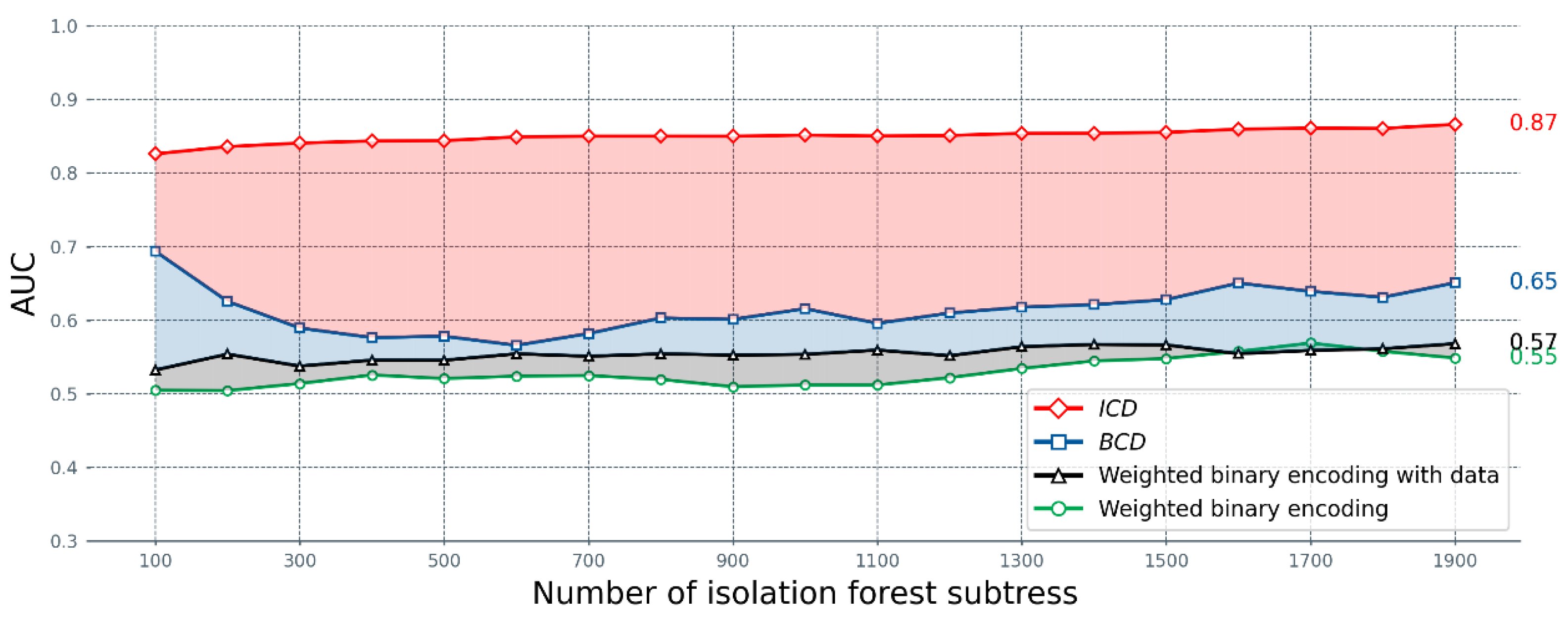
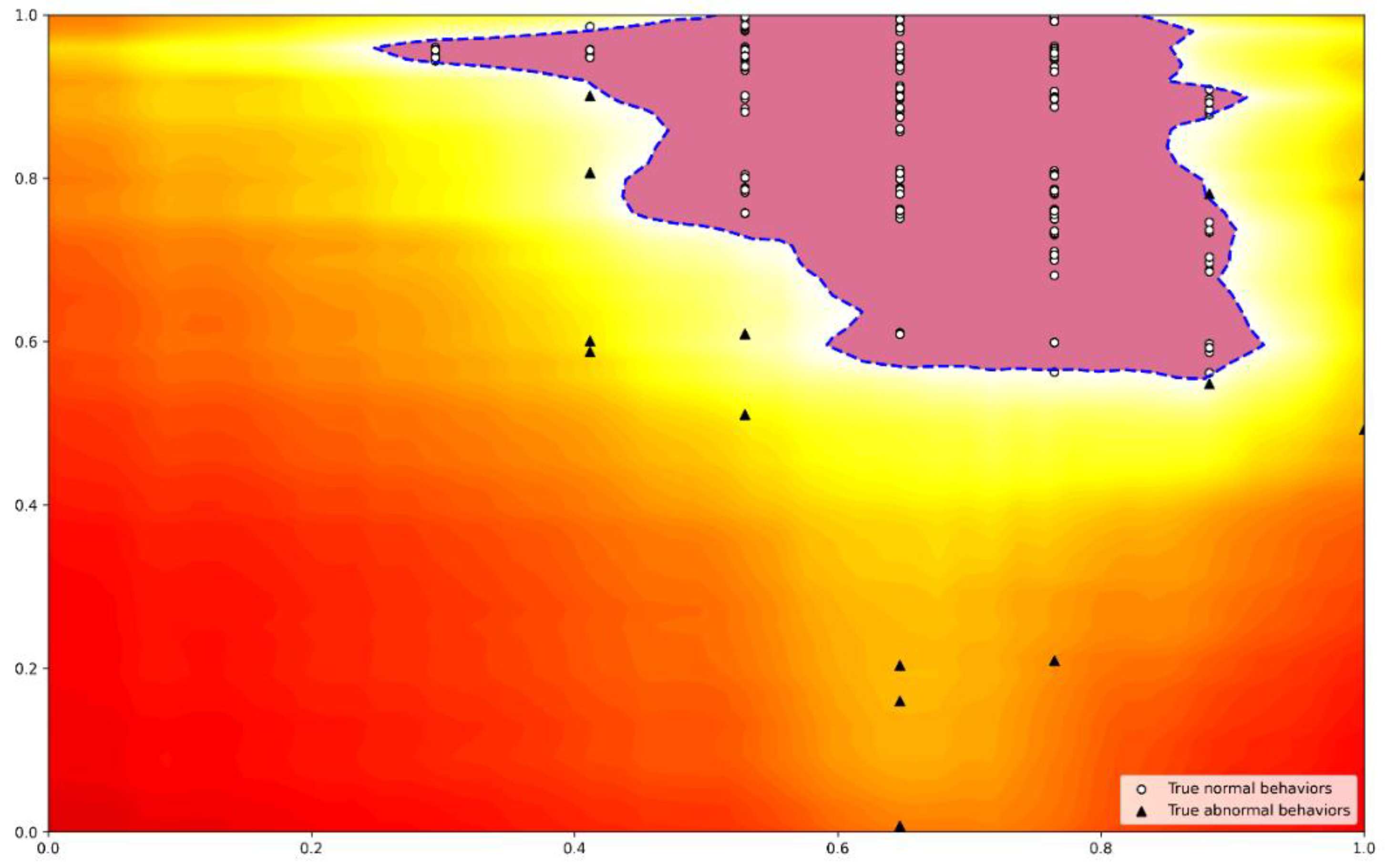
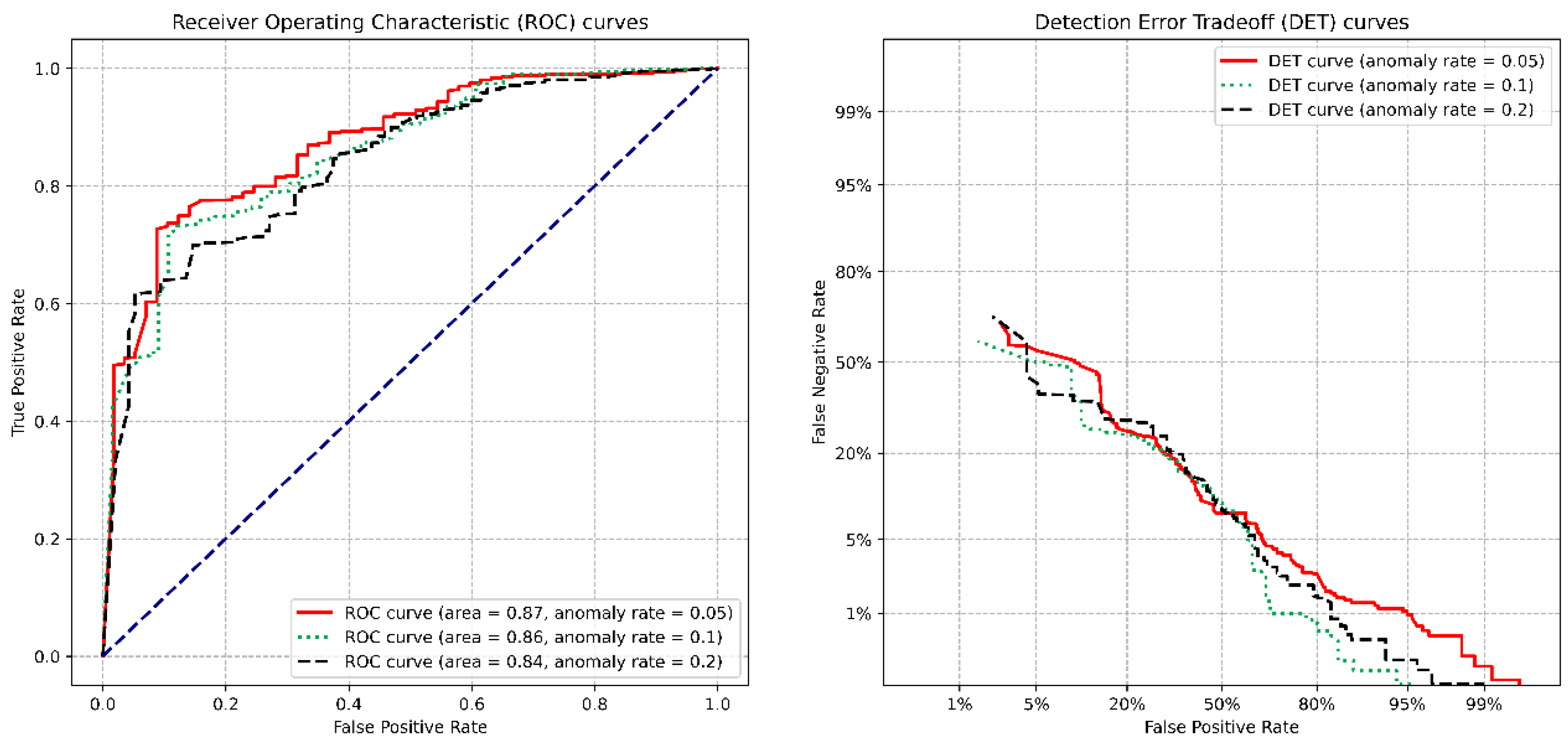
7.2. Experimental Results

Taking BPIC13_closed_problems as an example, this section analyzes in detail the detection capability of this paper’s algorithm for abnormal behaviors under different settings.

When only control flow constraints in events are considered, the number of features is small, and it is not easy to obtain better detection results. We take one of the subtrees of the isolation forest and plot it in Figure 7. At this time, the decision tree contains only one feature (i.e., x2), and the detection results are easily influenced by anomalous behavior, making it difficult to obtain accurate results.

The number of features and subtrees of the isolation forest is considered by increasing the number of features to improve the algorithm’s detection capability. Figure 8 shows the detection results of the isolation forest under different constraints, which include the control flow-based consistency measure BCD and the fused control flow and data flow consistency measure ICD. We also compare the constraints based on the One-hot encoding of activity and attribute features. During these evaluations, all other parameters were kept consistent. The results show that the detection results based on the integration consistency measure have high AUC values and the detection results show an increasing trend with a smoother increase. The detection results based on the behavioral consistency measure were the second highest, but the results fluctuated more. The detection results using One-hot coding have a minor numerical increase when adding data constraints, but the curve alignment is smoother than the curve considering only the control flow. Two conclusions can be drawn by combining the above four scenarios: (1) The detection results with attribute constraints are better than those considering only the control flow, which indicates that considering attribute constraints in the analysis process can improve the AUC value to some extent and increase the robustness of the detection results. (2) The anomaly detection results under the behavioral relationship of the fusion consistency characterization are better than those of the One-hot characterization, which indicates that the integrated consistency metric has improved discriminability.

We reduce the trace vector of the event log to a two-dimensional space, as shown in Figure 9. In this figure, the axis numbers indicate the coordinate components of the event log in this dimension. We use the blue dashed line to indicate the learned detection method. The contour line between the axes and the dashed line indicates the anomaly score plotted according to the trained detection algorithm. The normal trace vector is concentrated in the central region with a high detection score. While the trace vectors in the outer region further away from the blue dashed line have lower scores, i.e., anomalous behavior.

Figure 10 shows the ROC curve (left) and DET curve (right) of this log for detecting abnormal behavior by the algorithm in this paper when the abnormal threshold is 0.05 and 0.2. As can be observed from the ROC curve graph (the blue diagonal line in the ROC indicates that TPR = FPR, i.e., the model tends to predict at random.), the ROC curve of the algorithm is located in the dominant position when the percentage of abnormal behavior is 0.05. The highest AUC value is 0.87 at this setting, while the ROC curve is the next highest at the abnormal behavior ratio of 0.1 and 0.2. At this point, a comparison can be made with the help of the DET graph, which reflects the detection error rate, and the curve near the lower left corner indicates the strong recognition ability of the algorithm. Comparing the DET curves at an abnormal behavior rate of 0.1 and 0.2 reveals that the algorithm outperforms the results at an abnormal rate of 0.1 compared to 0.2. This indicates that the detection algorithm’s recognition ability decreases when the abnormal behavior content increases. We further infer that if there are enough abnormal behaviors, it will cause the system to have difficulty discriminating abnormal behaviors from normal behaviors. Therefore the anomalous behavior reduces the system’s robustness and the anomaly detection method proposed can effectively identify anomalous behavior and improve the system’s reliability.

Figure 11 compares various anomaly detection methods’ F1 scores and AUC values of different data sets. The results of multiple experiments show that the anomaly detection method based on the integrated consistency metric in this paper has the advantage of robustness in real logs. Specifically, (1) anomaly detection based on the integration consistency measure obtains high F1 scores and AUC values in all test logs. For example, in the Helpdesk and Sepsis logs, both metrics reach above 0.9. (2) Compared with other anomalous behavior detection methods under the same settings, the method in this paper significantly outperforms the DAE and OC-SVM methods, outperforms the BINet method in some cases, and only slightly underperforms the F1 score of BPI20PrepaidTravelCost and the AUC metrics of BPIC13_closed_problems in BINet.

8. Conclusions

A multi-view online model enhancement method fusing data and control flow is proposed. The method considers the effects of control flow-level behavioral relationships and data flow-level resource attributes in online scenarios and uses deep clustering and association rule mining methods for analysis, respectively. First, the reference model is analyzed to construct a multi-view hybrid confidence interval constraint in the offline phase. From the control flow perspective, the behavioral relationships among activities are studied using deep clustering methods. In addition, the resource co-occurrence relationship is analyzed based on association rules from the perspective of resource flow. Next, an incremental update algorithm for online scenarios is proposed to achieve model enhancement by filtering event streams and iteratively optimizing credible intervals. Finally, the proposed algorithm was implemented based on the PM4Py framework and the resulting model quality and execution efficiency were evaluated using real logs. The results of several sets of comparative experiments show that the algorithm improves the model’s robustness and obtains desirable results under noise interference.

In future work, we plan to improve the corresponding capability of the algorithm so that it can be applied to real-time scenarios. In addition, there are many threshold-setting scenarios for implementing isolation forests and the experimental results in this paper are the optimal values generated under many experiments. In the future, we will explore more efficient threshold-setting strategies to improve the efficiency and accuracy of the experiments.

References

1. Nolle, T.; Luettgen, S.; Seeliger, A.; Mühlhäuser, M. BINet: Multi-perspective business process anomaly classification. Inf. Syst. 2022, 103, 101458. [Google Scholar] [CrossRef] [Green Version]
2. Burattin, A.; Josep, C. A Framework for online conformance checking. In Business Process Management Workshops. In Business Process Management Workshops; Springer: Cham, Switzerland, 2018; Volume 308, pp. 165–177. [Google Scholar] [CrossRef] [Green Version]
3. Breunig, M.M.; Kriegel, H.-P.; Ng, R.T.; Sander, J. LOF: Identifying density-based local outliers. In Proceedings of the 2000 ACM SIGMOD International Conference on Management of Data—SIGMOD ‘00, Dallas, TX, USA, 15–18 May 2000; Association for Computing Machinery: New York, NY, USA, 2000; pp. 93–104. [Google Scholar] [CrossRef]
4. Christy, A.; Gandhi, G.M.; Vaithyasubramanian, S. Cluster Based Outlier Detection Algorithm for Healthcare Data. Procedia Comput. Sci. 2015, 50, 209–215. [Google Scholar] [CrossRef] [Green Version]
5. Pillutla, M.R.; Raval, N.; Bansal, P.; Srinathan, K.; Jawahar, C.V. LSH based outlier detection and its application in distributed setting. In Proceedings of the 20th ACM International Conference on Information and Knowledge Management—CIKM ’11, Glasgow, UK, 24–28 October 2011; Association for Computing Machinery: New York, NY, USA, 2011; pp. 2289–2292. [Google Scholar] [CrossRef] [Green Version]
6. Mannhardt, F.; de Leoni, M.; Reijers, H.A.; van der Aalst, W.M.P. Balanced multi-perspective checking of process conformance. Computing 2016, 98, 4. [Google Scholar] [CrossRef] [Green Version]
7. Sani, M.F.; van Zelst, S.J.; van der Aalst, W.M.P. Repairing Outlier Behaviour in Event Logs using Contextual Behaviour. Enterp. Model. Inf. Syst. Archit. (EMISAJ) 2019, 14, 115–131. [Google Scholar] [CrossRef]
8. Nolle, T.; Luettgen, S.; Seeliger, A.; Mühlhäuser, M. Analyzing business process anomalies using autoencoders. Mach. Learn. 2018, 107, 1875–1893. [Google Scholar] [CrossRef] [Green Version]
9. Bezerra, F.; Wainer, J. Algorithms for anomaly detection of traces in logs of process aware information systems. Inf. Syst. 2013, 38, 33–44. [Google Scholar] [CrossRef]
10. Genga, L.; Alizadeh, M.; Potena, D.; Diamantini, C.; Zannone, N. Discovering anomalous frequent patterns from partially ordered event logs. J. Intell. Inf. Syst. 2018, 51, 257–300. [Google Scholar] [CrossRef]
11. Van Zelst, S.J.; Bolt, A.; Hassani, M.; van Dongen, B.F.; van der Aalst, W.M.P. Online conformance checking: Relating event streams to process models using prefix-alignments. Int. J. Data Sci. Anal. 2019, 8, 269–284. [Google Scholar] [CrossRef] [Green Version]
12. Ghionna, L.; Greco, G.; Guzzo, A.; Pontieri, L. Outlier detection techniques for process mining applications. In Foundations of Intelligent Systems; Springer: Berlin, Heidelberg, Germany, 2008. [Google Scholar] [CrossRef]
13. Neto, R.V.; Tavares, G.; Ceravolo, P.; Barbon, S. On the use of online clustering for anomaly detection in trace streams. In Proceedings of the XVII Brazilian Symposium on Information Systems, Uberlândia, Brazil, 7–10 June 2021; ACM: Uberlândia, Brazil, 2021; pp. 1–8. [Google Scholar] [CrossRef]
14. Mozaffari, M.; Yilmaz, Y. Online Anomaly Detection in Multivariate Settings. In Proceedings of the 2019 IEEE 29th International Workshop on Machine Learning for Signal Processing (MLSP), Pittsburgh, PA, USA, 13–16 October 2019; IEEE: Pittsburgh, PA, USA, 2019; pp. 1–6. [Google Scholar] [CrossRef]
15. Laxhammar, R.; Falkman, G. Online Learning and Sequential Anomaly Detection in Trajectories. IEEE Trans. Pattern Anal. Mach. Intell. 2014, 36, 6. [Google Scholar] [CrossRef] [PubMed]
16. Böhmer, K.; Rinderle-Ma, S. Multi Instance Anomaly Detection in Business Process Executions. In Business Process Management; Carmona, J., Engels, G., Kumar, A., Eds.; Springer International Publishing: Cham, Switzerland, 2017. [Google Scholar] [CrossRef]
17. De Leoni, M.; Felli, P.; Montali, M. "Integrating BPMN and DMN: Modeling and Analysis. J. Data Semant. 2021, 10, 165–188. [Google Scholar] [CrossRef]
18. Tavares, G.M.; da Costa, V.G.T.; Martins, V.E.; Ceravolo, P.; Barbon, S. Anomaly Detection in Business Process based on Data Stream Mining. In Proceedings of the XIV Brazilian Symposium on Information Systems—SBSI’18, Caxias do Sul, Brazil, 4–8 June 2018; Association for Computing Machinery: Caxias do Sul, Brazil, 2018; pp. 1–8. [Google Scholar] [CrossRef]
19. Ebrahim, M.; Golpayegani, S.A.H. Anomaly detection in business processes logs using social network analysis. J. Comput. Virol. Hack. Tech. 2022, 18, 127–139. [Google Scholar] [CrossRef]
20. Van der Aalst, W.M.P. Process Mining: Data Science in Action, 2nd ed.; Springer: Berlin, Heidelberg, Germany, 2016. [Google Scholar]
21. Chan, N.N.; Yongsiriwit, K.; Gaaloul, W.; Mendling, J. Mining Event Logs to Assist the Development of Executable Process Variants. In Advanced Information Systems Engineering; Springer: Thessaloniki, Greece, 2014; Volume 8484, pp. 548–563. [Google Scholar] [CrossRef]
22. Polyvyanyy, A.; Smirnov, S.; Weske, M. Business process model abstraction. In Handbook on Business Process Management 1; Springer: Berlin, Heidelberg, Germany, 01 January 2014; pp. 147–165. [Google Scholar] [CrossRef]
23. Fang, X.; Wu, J.; Liu, X. An Optimized Method of Business Process Mining Based on the Behavior Profile of Petri Nets. Inf. Technol. J. 2013, 13, 86–93. [Google Scholar] [CrossRef] [Green Version]
24. Liu, F.T.; Ting, K.M.; Zhou, Z.-H. “Isolation Forest. In Proceedings of the 2008 Eighth IEEE International Conference on Data Mining; IEEE: Pisa, Italy, 19 December, 2008; pp. 413–422. [Google Scholar] [CrossRef]
25. Liu, F.T.; Ting, K.M.; Zhou, Z.-H. "Isolation-Based Anomaly Detection. ACM Transactions on Knowledge Discovery from Data 2012, 6, 1–39. [Google Scholar] [CrossRef]
26. Bloemen, V.; Van Zelst, S.; Van der Aalst, W.; Van Dongen, B.; Van de Pol, J. Aligning observed and modelled behaviour by maximizing synchronous moves and using milestones. Information Systems 2022, 103, 101456. [Google Scholar] [CrossRef]
27. Raschka, S. Python Machine Learning; Packt Publishing Ltd.: Birmingham, UK, 2015. [Google Scholar]
28. Mannhardt, F.; Blinde, D. Analyzing the Trajectories of Patients with Sepsis using Process Mining. RADAR 2017, 1859, 72–80. [Google Scholar]
29. Wressnegger, C.; Schwenk, G.; Arp, D.; Rieck, K. A close look on n-grams in intrusion detection. In Proceedings of the 2013 ACM Workshop on Artificial Intelligence and Security, Berlin, Germany, 4 November 2013; Association for Computing Machinery: New York, NY, USA, 4 November, 2013; pp. 67–76. [Google Scholar] [CrossRef]
Figure 1. Overview of research methods, inputs, and outputs.
Electronics 11 03640 g001
Figure 2. Petri net of insurance claim processes with data attributes of the activities.
Electronics 11 03640 g002
Figure 3. Division of sample points.
Electronics 11 03640 g003
Figure 4. K-order neighborhood.
Electronics 11 03640 g004
Figure 5. Attribute Matching.
Electronics 11 03640 g005
Figure 6. Possible movement when logs are aligned with models for properties.
Electronics 11 03640 g006
Figure 7. A subtree of the isolation forest when only the control flow constraint is considered.
Electronics 11 03640 g007
Figure 8. Effect of different numbers of subtrees on detection results.
Electronics 11 03640 g008
Figure 9. Distribution of data based on anomaly score contour.
Electronics 11 03640 g009
Figure 10. ROC and DET of Log BPIC2013_closed_issue.
Electronics 11 03640 g010
Figure 11. F1 score and AUC for all data sets in the detection methods.
Electronics 11 03640 g011