
A Method for Predicting the Remaining Life of Rolling Bearings Based on Multi-Scale Feature Extraction and Attention Mechanism
Abstract
:1. Introduction
2. Basic Theory
2.1. Convolutional Neural Networks
- (1)
- Input layer: utilized mainly for data entry.
- (2)
- Convolutional layer: It has the advantages of local area connectivity and weight sharing. The convolution layer is composed of a group of convolution kernels, which are the main tools for feature extraction. The specific operations are shown below.
- (3)
- Pooling layers: Generalize the output of convolutional layers at specific neighboring locations in the form of non-linear down-sampling to reduce the computational effort of the model, thereby increasing the computational speed of the network and making the feature representation translation invariant. This article adopts max pooling, the specific operations of which are shown below.
- (4)
- Fully connected layer: It maps the feature space extracted from the data after convolution and pooling to the sample space. The specific operations are shown below.
- (5)
- Output layer: mainly used to output the final prediction results.
2.2. Dilated Convolution
2.3. LSTM Networks
2.4. Attentional Mechanisms
3. Rolling Bearing RUL Prediction Based on Multi-Scale Feature Extraction and Attention Mechanism
3.1. Network Model Construction
3.2. Prediction Process of Bearing RUL Based on Multi-Scale Feature Extraction and Attention Mechanism
4. Test Validation
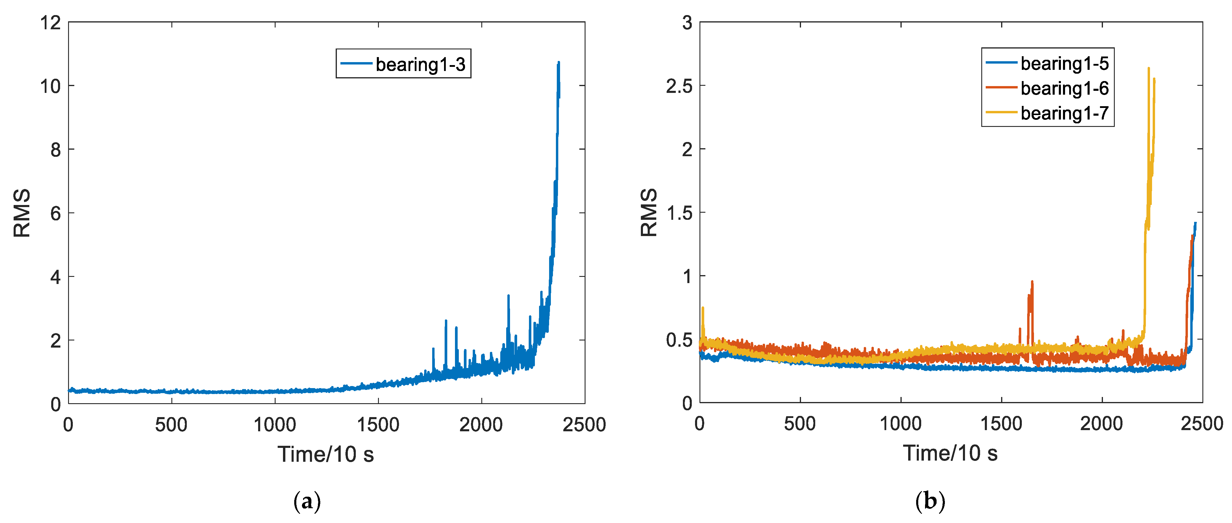
4.1. Test Data
4.1.1. Data Preprocessing
4.1.2. Construction of Data Labels
4.2. Evaluation Indicators
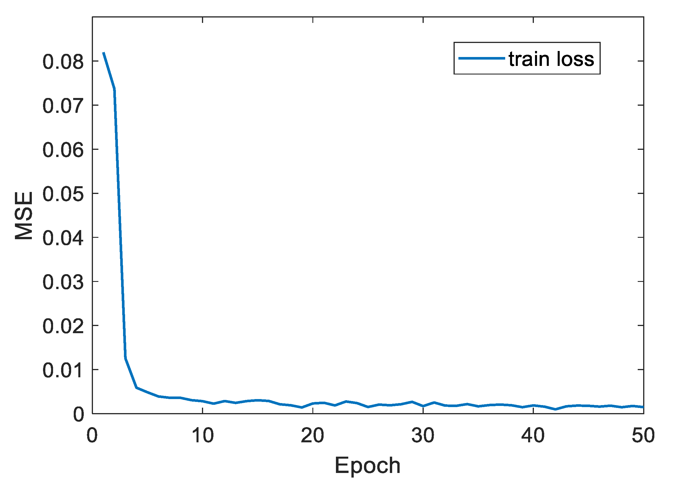
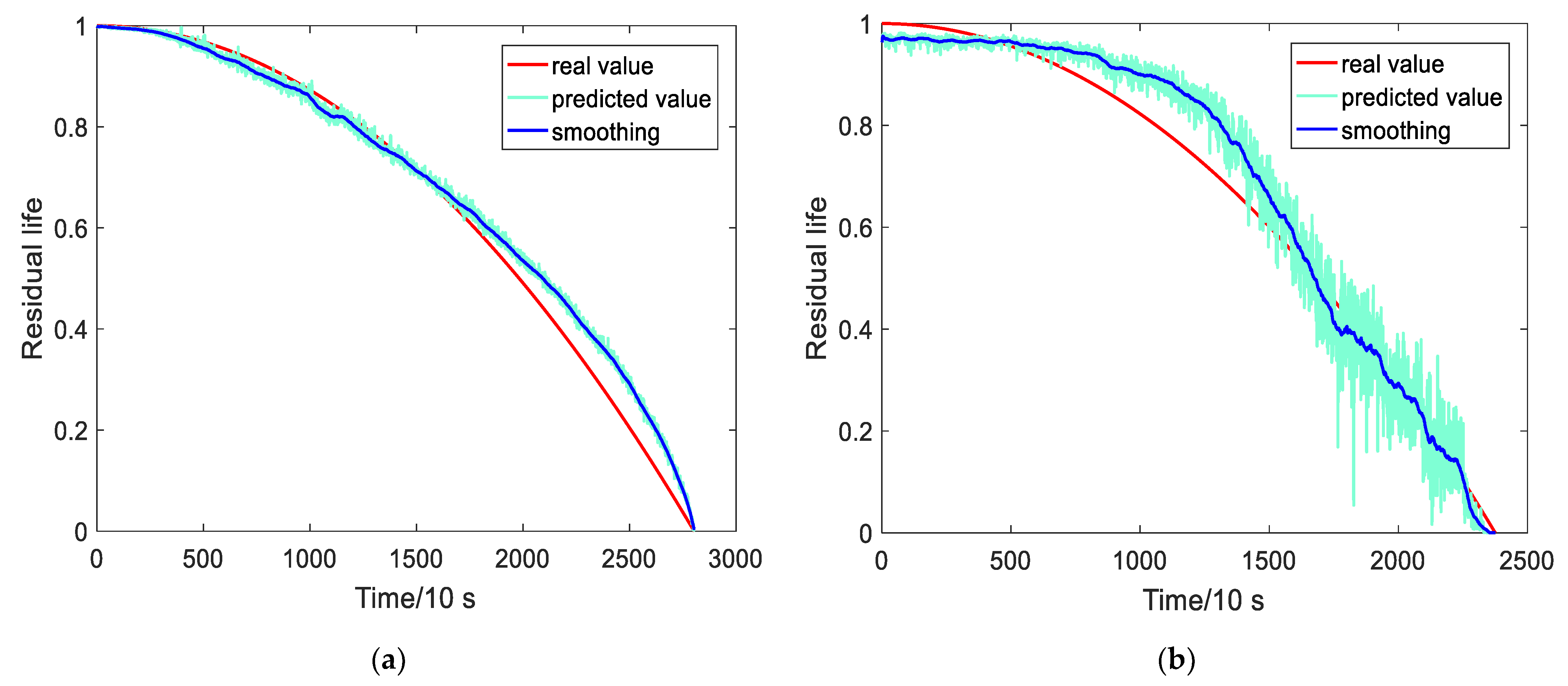
4.3. Test Results
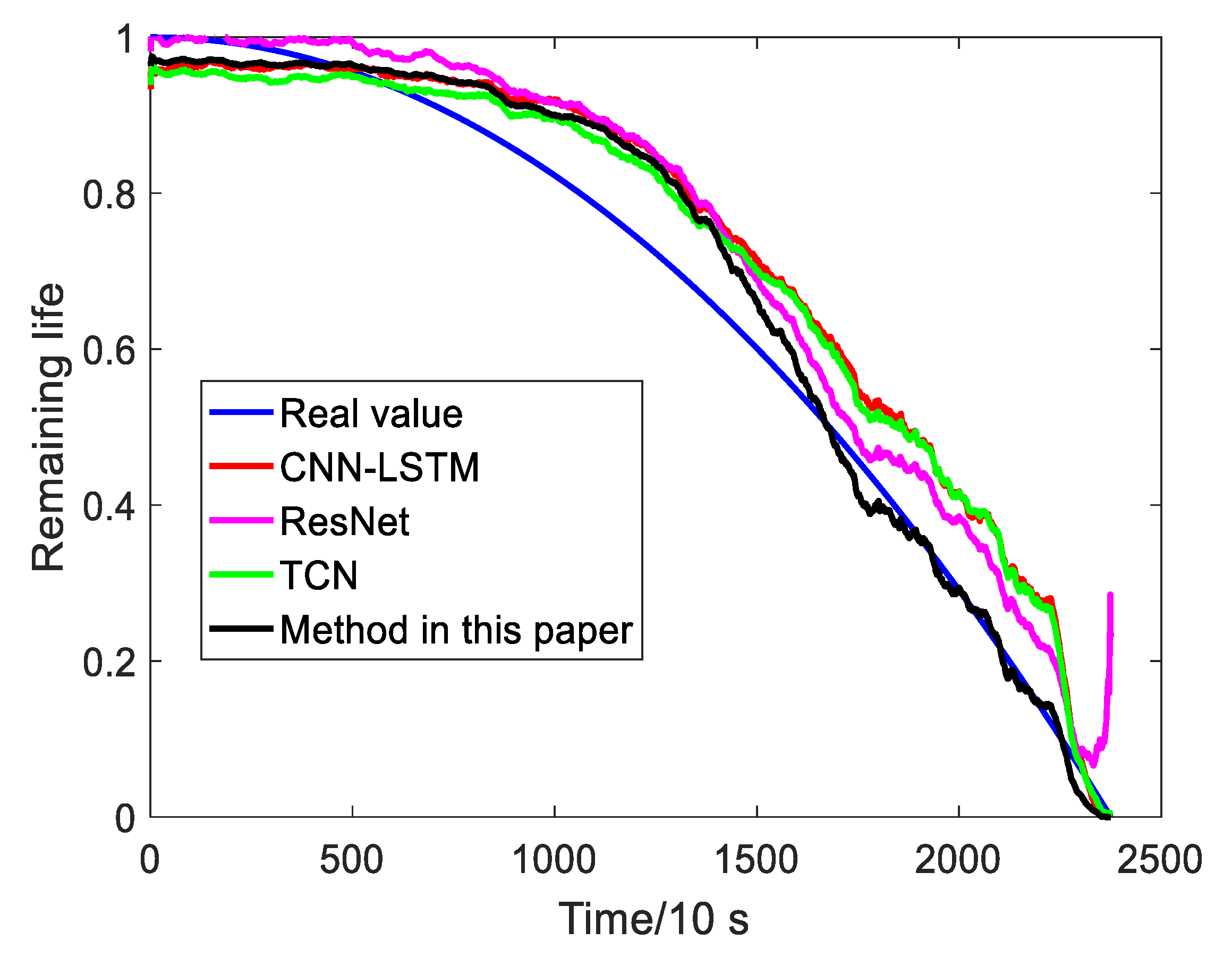
4.4. Comparison Test
5. Conclusions
Author Contributions
Funding
Institutional Review Board Statement
Informed Consent Statement
Conflicts of Interest
References
- Chen, C.-C.; Liu, Z.; Yang, G.; Wu, C.-C.; Ye, Q. An Improved Fault Diagnosis Using 1D-Convolutional Neural Network Model. Electronics 2020, 10, 59. [Google Scholar] [CrossRef]
- Gu, K.; Zhang, Y.; Liu, X.B.; Li, H.; Ren, M.F. DWT-LSTM-Based Fault Diagnosis of Rolling Bearings with Multi-Sensors. Electronics 2021, 10, 2076. [Google Scholar] [CrossRef]
- Zhu, J.; Chen, N.; Peng, W.W. Estimation of Bearing Remaining Useful Life Based on Multiscale Convolutional Neural Network. IEEE Trans. Ind. Electron. 2019, 66, 3208–3216. [Google Scholar] [CrossRef]
- Tian, Z.G.; Liao, H.T. Condition based maintenance optimization for multi-component systems using proportional hazards model. Reliab. Eng. Syst. Saf. 2011, 96, 581–589. [Google Scholar] [CrossRef]
- Xie, Z.; Du, S.; Lv, J.; Deng, Y.; Jia, S. A Hybrid Prognostics Deep Learning Model for Remaining Useful Life Prediction. Electronics 2020, 10, 39. [Google Scholar] [CrossRef]
- Zio, E.; Peloni, G. Particle filtering prognostic estimation of the remaining useful life of nonlinear components. Reliab. Eng. Syst. Saf. 2011, 96, 403–409. [Google Scholar] [CrossRef]
- Chen, C.C.; Zhang, B.; Vachtsevanos, G. Prediction of Machine Health Condition Using Neuro-Fuzzy and Bayesian Algorithms. IEEE Trans. Instrum. Meas. 2012, 61, 297–306. [Google Scholar] [CrossRef]
- Malhi, A.; Yan, R.Q.; Gao, R.X. Prognosis of Defect Propagation Based on Recurrent Neural Networks. IEEE Trans. Instrum. Meas. 2011, 60, 703–711. [Google Scholar] [CrossRef]
- Ren, L.; Sun, Y.Q.; Cui, J.; Zhang, L. Bearing remaining useful life prediction based on deep autoencoder and deep neural networks. J. Manuf. Syst. 2018, 48, 71–77. [Google Scholar] [CrossRef]
- Zhang, C.; Lim, P.; Qin, A.K.; Tan, K.C. Multiobjective Deep Belief Networks Ensemble for Remaining Useful Life Estimation in Prognostics. IEEE Trans. Neural Netw. Learn Syst. 2017, 28, 2306–2318. [Google Scholar] [CrossRef]
- Toldinas, J.; Venčkauskas, A.; Liutkevičius, A.; Morkevičius, N. Framing Network Flow for Anomaly Detection Using Image Recognition and Federated Learning. Electronics 2022, 11, 3138. [Google Scholar] [CrossRef]
- Cui, J.-W.; Du, H.; Yan, B.-Y.; Wang, X.-J. Research on Upper Limb Action Intention Recognition Method Based on Fusion of Posture Information and Visual Information. Electronics 2022, 11, 3078. [Google Scholar] [CrossRef]
- Liu, J.; Cong, R.; Wang, X.; Zhou, Y. Link-aware Frame Selection for Effificient License Plate Recognition in Dynamic Edge Networks. Electronics 2022, 11, 3186. [Google Scholar] [CrossRef]
- Guo, L.; Lei, Y.G.; Li, N.P.; Yan, T.; Li, N.B. Machinery health indicator construction based on convolutional neural networks considering trend burr. Neurocomputing 2018, 292, 142–150. [Google Scholar] [CrossRef]
- Wang, H.; Peng, M.J.; Miao, Z.; Liu, Y.K.; Ayodeji, A.; Hao, C. Remaining useful life prediction techniques for electric valves based on convolution auto encoder and long short term memory. ISA Trans. 2021, 108, 333–342. [Google Scholar] [CrossRef]
- Zhang, J.M.; Lu, C.Q.; Wang, J.; Wang, L.; Yue, X.G. Concrete Cracks Detection Based on FCN with Dilated Convolution. Appl. Sci. 2019, 9, 2686. [Google Scholar] [CrossRef] [Green Version]
- Wang, Y.J.; Wang, G.D.; Chen, C.L.Z.; Pan, Z.K. Multi-scale dilated convolution of convolutional neural network for image denoising. Multimed. Tools Appl. 2019, 78, 19945–19960. [Google Scholar] [CrossRef]
- Guo, L.; Li, N.P.; Jia, F.; Lei, Y.G.; Lin, J. A recurrent neural network based health indicator for remaining useful life prediction of bearings. Neurocomputing 2017, 240, 98–109. [Google Scholar] [CrossRef]
- Li, F.; Xiang, W.; Wang, J.; Zhou, X.; Tang, B. Quantum weighted long short-term memory neural network and its application in state degradation trend prediction of rotating machinery. Neural Netw. 2018, 106, 237–248. [Google Scholar] [CrossRef]
- Ma, M.; Mao, Z. Deep-Convolution-Based LSTM Network for Remaining Useful Life Prediction. IEEE Trans. Ind. Inform. 2021, 17, 1658–1667. [Google Scholar] [CrossRef]
- Tian, F.; Wang, L.; Xia, M. Signals Recognition by CNN Based on Attention Mechanism. Electronics 2022, 11, 2100. [Google Scholar] [CrossRef]
- Chen, Y.H.; Peng, G.L.; Zhu, Z.Y.; Li, S.J. A novel deep learning method based on attention mechanism for bearing remaining useful life prediction. Appl. Soft Comput. 2020, 86, 105919. [Google Scholar] [CrossRef]
- Wen, L.; Li, X.Y.; Gao, L.; Zhang, Y.Y. A New Convolutional Neural Network-Based Data-Driven Fault Diagnosis Method. IEEE Trans. Ind. Electron. 2018, 65, 5990–5998. [Google Scholar] [CrossRef]
- Yao, D.C.; Li, B.Y.; Liu, H.C.; Yang, J.W.; Jia, L.M. Remaining useful life prediction of roller bearings based on improved 1D-CNN and simple recurrent unit. Measurement 2021, 175, 109166. [Google Scholar] [CrossRef]
- Zhang, Z.; Wang, X.; Jung, C. DCSR: Dilated Convolutions for Single Image Super-Resolution. IEEE Trans. Image Process. 2019, 28, 1625–1635. [Google Scholar] [CrossRef]
- Spuhler, K.; Serrano-Sosa, M.; Cattell, R.; DeLorenzo, C.; Huang, C. Full-count PET recovery from low-count image using a dilated convolutional neural network. Med. Phys. 2020, 47, 4928–4938. [Google Scholar] [CrossRef]
- Wang, F.T.; Liu, X.F.; Deng, G.; Yu, X.G.; Li, H.K.; Han, Q.K. Remaining Life Prediction Method for Rolling Bearing Based on the Long Short-Term Memory Network. Neural Process. Lett. 2019, 50, 2437–2454. [Google Scholar] [CrossRef]
- Guo, R.X.; Wang, Y.; Zhang, H.C.; Zhanga, G.L. Remaining Useful Life Prediction for Rolling Bearings Using EMD-RISI-LSTM. IEEE Trans. Instrum. Meas. 2021, 70, 1–12. [Google Scholar] [CrossRef]
- Choi, H.; Cho, K.; Bengio, Y. Fine-grained attention mechanism for neural machine translation. Neurocomputing 2018, 284, 171–176. [Google Scholar] [CrossRef] [Green Version]
- Xu, X.W.; Wang, J.W.; Zhong, B.F.; Ming, W.W.; Chen, M. Deep learning-based tool wear prediction and its application for machining process using multi-scale feature fusion and channel attention mechanism. Measurement 2021, 177, 109254. [Google Scholar] [CrossRef]
- Singleton, R.K.; Strangas, E.G.; Aviyente, S. Extended Kalman Filtering for Remaining-Useful-Life Estimation of Bearings. IEEE Trans. Ind. Electron. 2015, 62, 1781–1790. [Google Scholar] [CrossRef]


| Working Condition | Condition 1 | Condition 2 | Condition 3 |
|---|---|---|---|
| Number of bearing | 1–1, 1–2, 1–3 | 2–1, 2–2, 2–3 | 3–1, 3–2, 3–3 |
| 1–4, 1–5, 1–6, 1–7 | 2–4, 2–5, 2–6, 2–7 | ||
| Load (N) | 4000 | 4200 | 5000 |
| Speed (r/min) | 1800 | 1650 | 1500 |
| Layers | Operating | Parameters Size |
|---|---|---|
| 1–1 | Convolution Dropout | Filter = 3, kernel_size = 5, dilation = 3 0.2 |
| Max-Pool | Pool_size = 2 | |
| Convolution | Filter = 6, kernel_size = 5, dilation = 3 | |
| Dropout | 0.2 | |
| Max-Pool | Pool_size = 2 | |
| 1–2 | LSTM | Hidden_size = 1500, num_layers = 2, dropout = 0.5 |
| 2 | Channel attention | / |
| Flatten | 5286 | |
| 3 | Fully connected 1 | 1000 |
| Fully connected 2 | 500 | |
| Fully connected 3 | 100 | |
| Fully connected 4 | 1 |
| Comparison Methods | CNN-LSTM | ResNet | TCN | Proposed Method | ||||
|---|---|---|---|---|---|---|---|---|
| Test Bearing | MAE | RMSE | MAE | RMSE | MAE | RMSE | MAE | RMSE |
| Bearing 1−3 | 0.0794 | 0.0981 | 0.0667 | 0.0814 | 0.0737 | 0.0851 | 0.0563 | 0.0705 |
| Bearing 1−4 | 0.1754 | 0.2311 | 0.2035 | 0.2789 | 0.1588 | 0.2140 | 0.1443 | 0.1689 |
| Bearing 1−5 | 0.3023 | 0.4151 | 0.3252 | 0.4335 | 0.3028 | 0.4146 | 0.2522 | 0.3467 |
| Bearing 1−6 | 0.2770 | 0.3850 | 0.2730 | 0.3772 | 0.2763 | 0.3845 | 0.2333 | 0.3089 |
| Bearing 1−7 | 0.2753 | 0.3801 | 0.2825 | 0.3849 | 0.2843 | 0.3968 | 0.2479 | 0.3455 |
Publisher’s Note: MDPI stays neutral with regard to jurisdictional claims in published maps and institutional affiliations. |
© 2022 by the authors. Licensee MDPI, Basel, Switzerland. This article is an open access article distributed under the terms and conditions of the Creative Commons Attribution (CC BY) license (https://creativecommons.org/licenses/by/4.0/).
Share and Cite
Jiang, C.; Liu, X.; Liu, Y.; Xie, M.; Liang, C.; Wang, Q. A Method for Predicting the Remaining Life of Rolling Bearings Based on Multi-Scale Feature Extraction and Attention Mechanism. Electronics 2022, 11, 3616. https://doi.org/10.3390/electronics11213616
Jiang C, Liu X, Liu Y, Xie M, Liang C, Wang Q. A Method for Predicting the Remaining Life of Rolling Bearings Based on Multi-Scale Feature Extraction and Attention Mechanism. Electronics. 2022; 11(21):3616. https://doi.org/10.3390/electronics11213616
Chicago/Turabian StyleJiang, Changhong, Xinyu Liu, Yizheng Liu, Mujun Xie, Chao Liang, and Qiming Wang. 2022. "A Method for Predicting the Remaining Life of Rolling Bearings Based on Multi-Scale Feature Extraction and Attention Mechanism" Electronics 11, no. 21: 3616. https://doi.org/10.3390/electronics11213616