Improving Path Accuracy of Mobile Robots in Uncertain Environments by Adapted Bézier Curves

Abstract

An algorithm that presents the best possible approximation for the theoretical Bézier curve and the real path on which a mobile robot moves in a dynamic environment with mobile obstacles and boundaries is introduced in this paper. The algorithm is tested on a set of scenarios that comprehensively cover critical situations of obstacle avoidance. The selection of scenarios is made by deploying robot navigation performances into constraints and further into descriptive characteristics of the scenarios. Computer-simulated environments are created with dedicated tools (i.e., Gazebo) and modeling and programming technologies (i.e., Robot Operating System (ROS) and Python). It is shown that the proposed algorithm improves the performance of the path for robot navigation in a highly dynamic environment, with dense mobile obstacles.

1. Introduction

A Bézier curve is a parametric curve, very well-known nowadays due to its multiple applications in science and engineering. It can approximate with high fidelity various forms found in nature and in society (medical image reconstruction [1], human organs [2], facial recognition [3], shape description [4], computer graphics and animation [5], traffic control [6], bus parking [7], automatic parking [8], path planning for robots [9,10,11,12,13,14,15,16,17,18,19], etc). Bézier curves were discovered by a French engineer named Piere Bézier [20]. He used them for the first time in designing Renault and Citroen cars to improve the aesthetics of the car’s shape [21].

Due to the increased interest in autonomous vehicle applications, in this paper, the authors introduce a Bézier curve-driven algorithm for improving mobile robot navigation. This research might be expanded to autonomous cars, too. However, initially testing such algorithms on less costly vehicles, such as mobile robots, is desirable. The major challenge is to prove that autonomous navigation driven by such algorithms among fixed and mobile obstacles is carried out safely, without collisions, and smoothly. Up to this moment, the scientific literature reports a variety of developments in the field of robot path planning [22,23,24,25], etc.

To focus the research from this paper, investigations for documenting the state of the art were conducted using Clarivate Analytics and Scopus. Past research was collected using the keyword “path planning”, which returned 5945 independent titles. The investigation was refined by looking inside this set with the keyword “Bézier curves”. The range of articles narrowed to 260. This resulting subset was analyzed, and it was concluded that the articles introduced in the next section are relevant to the purpose of this work.

2. Background

According to [26], there are algorithms used to solve path-finding problems by means of heuristic methods (the Dijkstra algorithm, A* algorithm [27], D* algorithm [28], and Lee algorithm [29]), meta-heuristics, random methods, and the hybrid components of these methods. The research from [30] provides information about a new parametrization of motion primitives for wheeled mobile robots. A parametrization of third-order Bézier motion primitives with continuous curvature (i.e., $C^2$ geometric curve continuity) in the joints is proposed. The primitive is computed as a solution that satisfies the boundary conditions for the position, orientation, and curvature at the endpoints. Besides the $C^2$ continuity, the primitive has several improvements: computational efficiency, minimal curve oscillations, and better convergence when applied to planning optimizers. These previous properties result from choosing a low-order primitive. The instructions for constructing primitives and an algorithm that connects the given way-points with the primitives resulting in a $C^2$ path are provided. The practical applications of the proposed primitives should be tested. An example of such applications is using the algorithm for a path optimizer for minimal-time safe path planning in a warehouse under variable load.

Article [31] proposes a new approach for autonomous mobile robots to solve path-planning problems by optimizing paths generated by random and traditional algorithms with Bézier curves in an environment full of known obstacles in every aspect. The proposed approach is applied in four stages: 1. The environment map consists of a grid. The cells which correspond to the obstacles, start, and endpoints are marked. 2. A path is computed from the previous map. This path begins from the starting point to go to the destination point. The Lee algorithm or the RRT algorithm (Rapidly Exploring Random Tree) are used to find the shortest path. 3. The raw path computed at step 3 contains too many nodes, so it needs to be pruned. The pruning is performed using linear Bézier curves, with the result of eliminating the extra nodes. 4. Along the path, the Spike nodes are smoothed using quadratic Bézier curves to create a safe path by ensuring the continuity of the path. After the four stages are run, the planned path between the starting point and the target point has the properties of being smooth, having a minimal length, and having a limited curvature. The simulation holds results that confirm the performance of the proposed stages. In this article, achieving success depends on knowing the environmental conditions.

The technique from [32] uses third-order Bessel curves and an improved artificial fish swarm algorithm. First, the morphological processing, such as the expansion of obstacles, is carried out. During the path-planning process, an artificial fish swimming range of 16 directions and 24 fields based on Dijkstra’s algorithm is run. The algorithm provides the movement rules of the artificial fish, which improves the accuracy of planning while reducing the number of inflection points. By adding the sharing mechanism, the number of operations of the fusion algorithm is reduced. The problem of mutual interference between the optimal local solution and the optimal global solution is solved. A feedback field of view is used, which limits the typically large field. Thanks to that, the oscillation phenomenon caused by an excessively large field of view in the later stage of the algorithm is avoided. The improved artificial fish swarm algorithm proposed in this paper generates a collision-free, inflection-point-less, and shorter path connected by a sequential sequence of path points. Finally, the continuity of the direction and curvature is smoothed by the use of cubic Bessel curves. The use of cubic Bessel curves also satisfies the minimum rotation radius to reduce the mechanical structure damage of the robot. By comparing the simulation results of the proposed algorithm with the traditional fish swarm algorithm, it can be observed that the proposed fusion algorithm has a shorter average path, fewer inflection points, and is more consistent with the kinematic characteristics of the robot while also ensuring a $100\%$ correct planning rate. At the same time, the proposed fusion algorithm makes use of Dijkstra’s algorithm, which causes an increase in computation, but the fish-sharing mechanism offsets part of the computation.

A different strategy is observed in [33]. It combines the continuous high-degree Bézier curve with an improved particle swarm optimization (PSO) algorithm. Compared with the other articles’ smooth path-planning approaches, the proposed strategy improves the smooth path planning of mobile robots. On the one hand, the smooth paths created via the continuous high-degree Bézier curve are “smoother” than those composed of several low-degree Bézier curve segments. The cause is that the high-order continuity (e.g., the continuous curvature derivative) can be naturally satisfied along the smooth path composed of a continuous high-degree Bézier curve. The smooth path obtained using the new strategy is also optimal because the continuity requirements are connected directly to the optimization criteria rather than inking several smooth curve segments. To deal with the complex optimization problem of the continuous high-degree Bézier curve, an improved PSO is suggested to overcome the frequently encountered problems of local trapping and premature convergence. By introducing an adaptive fractional-order velocity into the velocity updating function according to the state of the particle swarm evolution, some “disturbances” will be brought to the particle swarm. As such, some “power” will make it more likely to jump out of the local minima to explore and exploit the searching space more thoroughly. Thus, the problems of local trapping and premature convergence can be significantly improved. The advantages of the improved PSO algorithm were verified by the comparison of several standards and modified PSO algorithms, and the proposed algorithm was tested on several well-known standard benchmark functions. The improvement of the new strategy takes effect by solving the formulated optimization problem. This also has been confirmed by the smooth plan resulting during the simulations.

The authors intend to test the convergence of the algorithm with the help of computing the weight coefficients of the fractional-order velocities in a parameter domain. Moreover, they will test the performance of the improved PSO in other cases, such as the switching delay, the randomly distributed delay, the sigmoid-function-based adaptive weight, and the Markovian state jumping.

A chaotic particle swarm optimization (CPSO) algorithm to optimize the control points of the Bézier curve is proposed in [34]. The control points of the Bézier curve have an essential impact on discovering the optimal smooth path that minimizes the total distance between the starting and ending points. The proposed algorithm is created in two variants: CPSO-I and CPSO-II. Four experiments were conducted in this article. The first experiment observed the results of the two proposed algorithms using different chaotic maps. The results of this experiment share that the Singer and Sine maps were suitable for both algorithms. The second experiment compared the CPSO-I, CPSO-II, and PSO algorithms. The results of the second experiment revealed that (1) the CPSO-II algorithm achieved the best results and (2) replacing random parameters with chaotic maps in the PSO algorithm improved the performance of the PSO. The influence of the number of control points was tested in the third experiment. The results proved that increasing the number of control points increases the search space by adding extra dimensions. Therefore, a large population for the PSO is required to scan the search space perfectly. In the last experiment, the CPSO-II algorithm was tested against different numbers of obstacles, and the results proved that increasing the number of obstacles increases the problem’s difficulty. However, the proposed algorithm found the optimal path in most cases. The experiments in this paper were performed using only a static environment. However, a dynamic environment, i.e., moving obstacles, should be tested in the future to verify and extend the proposed algorithm. Searching for the optimal path in a three-dimensional environment should be tested in the future to simulate real robots’ movements, too.

Article [9] presents smooth route planning for mobile robots based on a Bézier quartic transition curve and an improved particle swarm optimization (PSO) algorithm. A new approach combined with a parametric cubic Bézier curve (PCBC) and particle swarm optimization with adaptive delayed velocity (PSO-ADV) algorithms is developed to plan the smooth path of mobile robots. The smooth path composed of PCBC segments can achieve an equivalent curvature at the joints of the segments, and thus it is able to attain a continuous curvature along the whole smooth path. Based on the mathematical formulation of the smooth path-planning problem, the optimal smooth path can be obtained by regulating the control points and control parameters of the PCBC, which is essentially an intractable optimization problem. Therefore, it is necessary to tackle this optimization problem and some frequently encountered troubles (e.g., the premature convergence and local trapping). A new PSO-ADV algorithm is developed, and by adding an adaptive delayed velocity term that can give the particles more “power’’ to jump out of the local minima, the validity of the PSO-ADV can be affirmed because of some simulation experiments on several famous benchmark functions. The advantages of this method are validated by running several experiments. The authors intend to work in the future on (1) the convergence analysis of the PSO-ADV algorithm; (2) the new schemes that can be employed to boost the performance of the PSO; and (3) the applications of the new smooth path-planning approach which cover some more complicated cases, e.g., 3D path planning, multi-robot path planning, and path planning in a severe environment.

The articles [35,36] present the Timed Elastic Bands (TEB) planner. It is an extensively used local planner for complex environments. It is integrated into the Robot Operating System (ROS) [37]. The TEB were formulated in [38]. The TEB planner is employed to efficiently and rapidly estimate a discretized trajectory in the plan. Formulated as a multi-objective optimization problem, the TEB planner takes into account constraints, such as the path feasibility from a robot’s kinematics point of view, velocity limits, and obstacle avoidance. Ref. [39] showcases situations when the TEB planner can be improved, such as a curve detour, acceleration strategies, and slight trajectory oscillations.

The article [30] presents one of the few, if not the first approach that uses cubic Bézier curves to discover motion primitives. To be able to use the primitives above, the given requirements for the initial and final position, orientation, and curvature are taken into account. A new parametrization method and an algorithm for computing the curve are introduced. The input pieces of information are the position, orientation, and curvature of the final output points. The proposed way of solving the problem consists of solving a system of two quadratic polynomial equations without the need for optimization. It is, therefore, computationally very efficient. While the initial information is needed, the authors use the hypothesis that the designer has access to a set of points interpolated into the final result. The final algorithm offers useful guidelines for choosing the right points and also for choosing the orientation of the resulting curve.

Article [40] describes a trajectory optimization of an automatic spraying robot. A large number of past articles proved that the initial trajectory of spray paint has a big influence on the final result of the painting operation with regard to thickness and uniformity. The results show that the operating time shrinks, the spray-painting efficiency increases, and the paint waste decreases. The optimal initial trajectory is classically selected using the plane-cutting method based on the cross-line cutting. It was determined that the U-direction and the V-direction could both satisfy the requirements after optimizing the robot’s course. That is, the thickness error is within the allowable error interval. However, the U-direction method turned out to hold better results, and the spray-painting efficiency was higher. It is mentionable that the shape of the work surface and the direction of the painting path influence the result. Therefore, both of them should be fully considered to increase efficiency. Firstly, the optimal initial trajectory of the spray-painting robot is chosen according to the features of the Bézier triangular surface. Secondly, the paint thickness is mathematically using the points from the Bézier surface. Finally, the trajectory along the Bézier surface is optimized using the ideal point method with the uniformity of the paint thickness. Another optimization objective used in the second step is the shortest spray-painting time. The proposed method has the advantage that it automatically determines an optimal path before the beginning of the spraying process, therefore significantly improving the uniformity of the coating thickness. Finally, a spraying experiment proves the effectiveness and practicability of the method.

Article [41] describes how a motion skill learning algorithm was proposed for a quadruped robot. The algorithm helps with the motion planning and stable walking of the quadruped robot on 5° and 11° slopes. First of all, the terrain slope is estimated using a proposed algorithm: the slope was estimated in relation to the robot’s foothold, which proved sufficient for computing the desired body attitude angle. Subsequently, the augmented random search (ARS) algorithm is used to develop a motion strategy for the quadruped, which is sufficiently open so that the quadruped robot easily adjusts its attitude to generate the desired body attitude. The Bezier curve was used to parameterize the trajectory, increasing the learning speed. Experiments were run inside a simulation, and the feasibility and effectiveness of the proposed framework held positive results. The robot adaptively adjusted its attitude and followed a correct motion on the slope, proving the required steadiness. To further validate our algorithm, the authors plan to transition the experiments to the real world for their future work.

As presented in the previous paragraphs of this review section, there is relevant research on mobile robot path planning, including some based on Bézier curves. However, microscopic research is reported on how to create a navigation route that is both collision free and time efficient in a highly dynamic navigation environment. We use Bézier curves with the Casteljau algorithm in this exploratory research to tackle the problem. The next section of the paper introduces the mathematical foundation of the Bézier curves, with adaptations to be easily replicable for any mobile robot, and the methodology for deploying navigation performances into comprehensive use cases.

3. Materials and Methods

3.1. Technical Prerequisites for the Proposed Method

The mathematical form for the Bézier curves is introduced in the next paragraphs of this section.

In ref. [42], a Bézier curve of degree n is represented as:

$$P_{[t_0,t_1]}\left(t\right)=\sum _{i=0}^n{B}_i^n\left(t\right)P_i,$$

(1)

where $P_i$, $i=1,\dots ,n$ are control points, such that $P\left(t_0\right)$ = $P_0$, $P\left(t_1\right)=P_n,\mathrm{and}{B}_i^n\left(t\right)$ is a Bernstein polynomial given by:

$$B_i^n={(}_i^n){\left(\frac{t_1-t}{t_1-t_0}\right)}^{n-i}{\left(\frac{t-t_0}{t_1-t_0}\right)}^i,i\in \{0,1,\dots ,n\},$$

(2)

where t denotes the time variable.

The Bézier curve has properties for path planning, as follows:

• Bézier curve always passes through $P_0$ and $P_n$;
• Bézier curve is always tangent to the lines connecting $P_0\to P_1$ and $P_n\to$$P_{n-1}$ at $P_0$ and $P_n$, respectively;
• Bézier curve always lies within the convex hull consisting of its control points.

In relation to the Bézier curves for mobile robot path planning, the Casteljau algorithm is relevant in the view of the authors of this paper [42]. The Casteljau algorithm describes a recursive method to subdivide a Bézier curve $P_{[t_0,t_2]}\left(t\right)$ into two segments $P_{[t_0,t_1]}\left(t\right)$ and $P_{[t_1,t_2]}\left(t\right)$.

Let denoting with $\{P_0^0,P_1^0,\dots ,P_n^0\}$ the control points of $P_{[t_0,t_2]}\left(t\right)$. The control points of $P_{[t_0,t_1]}\left(t\right)$ and $P_{[t_1,t_2]}\left(t\right)$ can be computed by:

$$P_i^j=(1-\tau )P_i^{j-1}+\tau P_{i+1}^{j-1},j\in \{1,\dots ,n\},i\in \{0,\dots ,n-j\},$$

(3)

where $\tau =\frac{t_1-t_0}{t_2-t_0}$. Then, $\{P_0^0,P_0^1,\dots ,P_0^n\}$ are the control points of $P_{[t_0,t_1]}$ and $\{P_0^n,P_1^{n-1},\dots ,P_n^0\}$ are the control points of $P_{[t_1,t_2]}$.

A Bézier curve $P_{[t_0,t_2]}$ always passes through the point $P\left(t_1\right)=P_0^n$ by applying the Casteljau algorithm to subdivide itself into $P_{[t_0,t_1]}$ and $P_{[t_1,t_2]}$. Moreover, it is always tangent to $\overline{P_0^{n-1}{P}_1^{n-1}}$ and $P\left(t_1\right)$.

The path-planning method introduced by the authors of this paper is motivated by the mathematical facts above. The robot’s path will be modeled by Bézier curves which use the obstacles as waypoints.

The Computational Geometry domain is also necessary for a number of steps from the authors’ final algorithm. Methods for checking the position of points relative to polygons, sorting points by special criteria, and simpler algorithms, such as Euclidean distance, are all employed inside the authors’ algorithm. Therefore, for further curiosities in Section 4 and Section 5, which present the proposed algorithm, it is recommended to see [43].

3.2. Brief Description of the Proposed Algorithm and Its Importance

The materials and methods described in the previous subsection above are deployed in the proposed algorithm: the authors developed a local planner based on Bézier curves. The proposed algorithm consists of using the fixed and mobile obstacles as waypoints inside the classical Bézier curves and enhancing the algorithm using geometrical artifices. For selecting and ordering the waypoints, the authors used the D* Lite algorithm to compute the optimal path. The obstacles that are closest to the optimal path were used as waypoints, but only after their positions are ordered by the time at which the guided robots will theoretically surpass each waypoint’s current positions.

The authors discovered that using the obstacles as waypoints is a good starting point, but it is not sufficient for the prevention of collisions. Through experimental simulations, the algorithm was enhanced by adapting the Bézier curves.

The adaptations are based on using the obstacles’ predicted positions rather than the current position. The choice has two useful results:

• Collisions can be detected a number of seconds before they happen, therefore offering the guided robot the choice between stopping and switching to a new route. The current route is considered wrong if the trajectory of the obstacle collides with the trajectory of the guided robot, or if following the current route would result in a critical distance between the robot and the obstacles.
• The predicted positions can be adapted to enhance the safety of the path. Let us consider that the guided robot has to surpass two relatively close mobile obstacles. Both obstacles are moving at a distance of less than 2 m to the guided robot. If one of the obstacles slightly approaches the guided robot, meaning that the distance between these two decreases, the waypoint which corresponds to the closest obstacle can be adapted. Gradually moving the more dangerous waypoint, the one which is closest to the guided robot, toward the less dangerous waypoint, the Bezier curve gradually balances the distance toward both closest obstacles.

More exactly, the space between the guided robot and the more dangerous mobile obstacles is increased by gradually moving the waypoints toward the fixed or less dangerous waypoints, consequently increasing the safety of the planned path.

The proposed method has the advantage of applicability for any mobile robot type and requires no identification of further parameters of mass, mass distribution, etc. These extra parameters are taken out of the equation because the authors used significant instances for the controllable parameters, instances that take into account critical values of perturbation factors.

3.3. Developing Real-World Simulation Stages for Path-Planning Use Cases

To test the performance of the proposed algorithm, a two-phase deployment function is further considered. It operates with three categories of parameters: performance indicators for navigation, constraints associated to the navigation environment, and comprehensive use cases (capable to cover all constraints). The first phase of deployment translates the performance indicators into constraints. This process will reveal if performances and constraints are properly related to each other. A relationship matrix (also called a connection matrix here) is used to perform deployment. Further, a set of navigation uses cases (here called scenarios) are imagined. Because we do not a priori know the comprehensiveness of the set of scenarios relative to the imposed constraints, deployment of constraints into scenarios is necessary. A connection matrix between constraints and scenarios is also adopted for this task. It reveals which scenarios are relevant and which can be rejected, as well as if there are some drawbacks in the definition of the current set of scenarios such that some of the scenarios to be improved or new scenarios to be designed and added to the set.

For this research, the following performance indicators are considered in relation to the navigation process in simulations:

• $P_{erf1}$: navigation speed (maximum target 1.6 m/s);
• $P_{erf2}$: vital navigation space (minimum target 30 × 30 cm);
• $P_{erf3}$: planned curve tolerance (maximum target 3–15 cm).

For other applications, the set of performance indicators can be expanded, modified, etc. This gives a character of generality to our methodology. For the practical problems taken into account in this research, the following constraints have been selected:

• C1: the obstacles width and height (maximum target width × height: 600 × 500 mm);
• C2: the velocity of the mobile obstacle (target 0.85 m/s, there were also videos with 1.8 and 1 m/s);
• C3: the direction of the mobile obstacles: straight lines with 90-degree edges;
• C4: the shape of the boundaries of the maneuvering space: rectangular space;
• C5: the density of the fixed obstacles: 6 and 9 depending on scenario;
• C6: the density of the mobile obstacles: 1, 5, 10, 15 obstacles, depending on scenario;
• C7: the direction of the mobile obstacles as compared to the robot’s direction: perpendicular, tangent, parallel.

The set of constraints can be altered for other practical cases. This indicates the general character of the proposed methodology. The authors use the symbols of performance indicators $P_{erf1},P_{erf2},P_{erf3}$ and constraints $C_1,C_2,C_3,C_4,C_5,C_6,C_7$ to visualize the deployment process. It is shown in

Table 1. Connection matrix. This connection matrix describes the dependency between constraints and performance indicators. The numbers are selected based on simulations’ visual results.

	C1	C2	C3	C4	C5	C6	C7
P${}_{erf1}$	1	9	3	9	3	9	3
P${}_{erf2}$	9	3	3	9	9	3	9
P${}_{erf3}$	1	9	9	3	0	9	9

, where values 9, 3, 1, and 0 have the following meanings:

• Strong connection between the constraint and performance indicator = 9;
• Average connection between the constraint and performance indicator = 3;
• Weak connection between the constraint and performance indicator = 1;
• No connection between the constraint and performance indicator = 0.

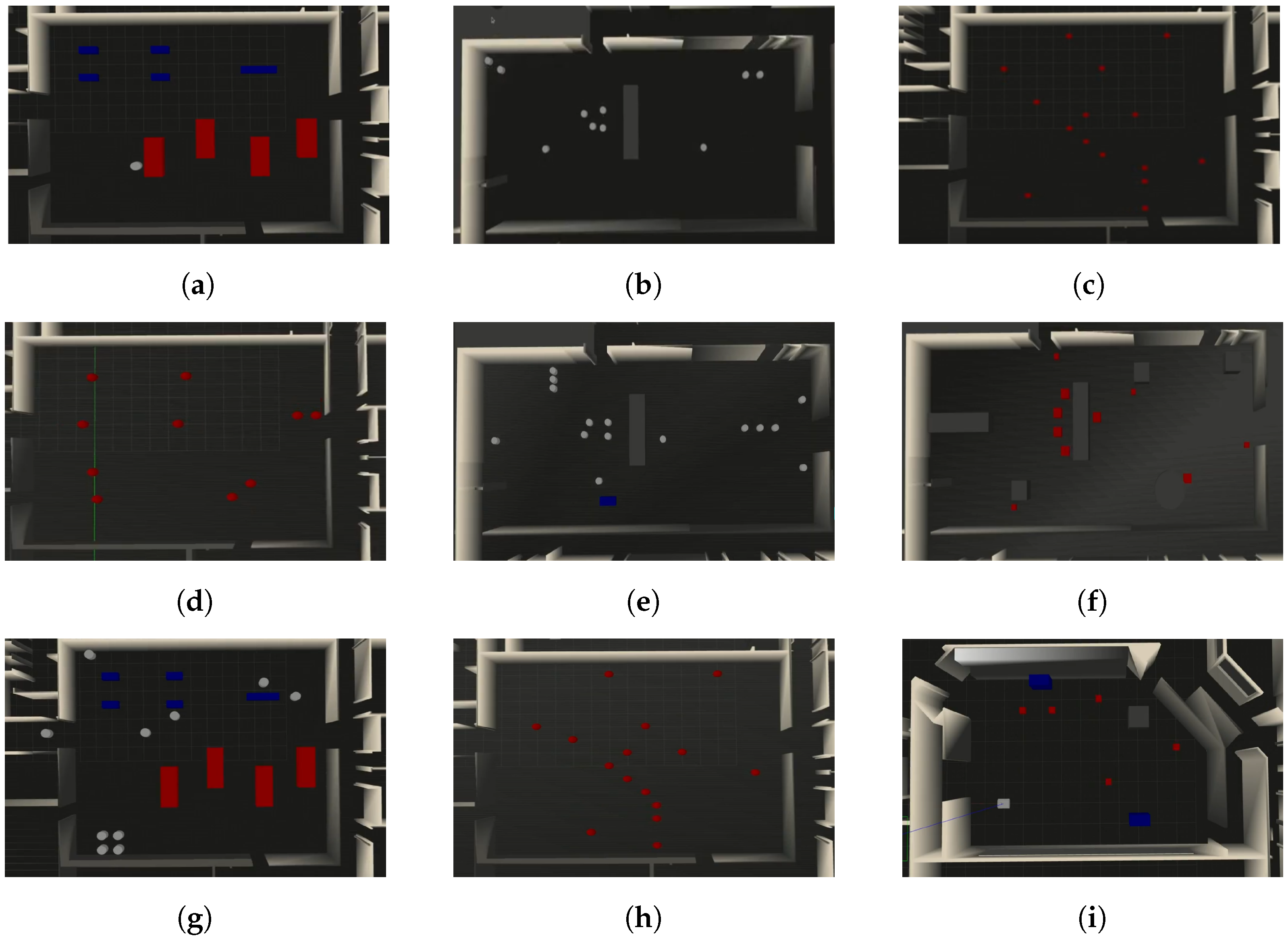
As data in Table 1 indicate, the authors see at least a strong connection (value 9) on each row and on each column; therefore, the authors conclude that the set of constraints is adequate and sufficient to deploy the performance indicators into practical use cases (generically described by the set of constraints).

Not having the possibility to establish on an analytical, quantitative basis the right package of scenarios, the authors propose here a new technique. A number of scenarios are firstly imagined by considering real-life situations where the robot will have to operate. Further, these scenarios are evaluated with respect to the set of constraints. Only scenarios that have at least a strong connection with at least one constraint will be kept. The final set can be further refined by eliminating some of the remaining scenarios that do not provide unique characteristics with respect to the others, and by this process, the above-mentioned rule of strong relationships along the rows and columns is not affected. It might happen that some constraints suffer of strong relationships with the set of scenarios. In this case, new scenarios must be imagined and tested until the problem is fixed.

Based on this idea, scenarios (also called here stages) are inspired from real-life cases (e.g., office building, school, supermarket, etc.). The proposed scenarios (stages) in this paper capture obstacles associated with actors (i.e., adults, children, other robots) located in different environments (schools, library, supermarket, etc.) and in different contexts (e.g., different distances related to the tested mobile robot, various speeds and movement directions of the obstacles). A variable number of obstacles are considered for each scenario, too. In this research, the authors started with the consideration of sixteen stages.

The full description of the sixteen stages is listed in

Table 2. The full description of the simulations created in Gazebo.

The 1st Stage	At the library, a person inspects the shelves, stops, chooses a book, moves to the book registration area, and leaves the room.
The 2nd Stage	Director’s room. A syrup bottle fell and broke in the middle of the room. Two robots are wet vacuuming, two robots are dry vacuuming, and a robot cleans the hard-to-reach areas of the room.
The 3rd Stage	Ten children develop various skills in a room specially set up for them. They run, tell stories in a group, and play various games.
The 4th Stage	Fifteen robots carry documents and perform various other tasks. The difficulty of this route consists of the large number of robots and their variable paths. Some of the robots stop because they have completed their tasks while others continue to work.
The 5th Stage	At the conference room, obstacles are represented by a person talking on the phone, a group of three people who talk during the break and then return to their seats, and three speakers. The people that do not leave the seats represent the fixed obstacles while the other people are mobile obstacles.
The 6th Stage	Ten cleaning robots are performing various tasks in a room currently under renovation. They all follow different paths over different distances.
The 7th Stage	The day before vacation. The gym will be closed in ten minutes, and there will be only five children. Two are taking the running test. Furthermore, the other three are doing group exercises.
The 8th Stage	The robot replenishes the stocks of perfumes for the four tables. In order to fulfill the objective of having all eight types of obstacles in the same sequence, the robot starts its activity in the space between the perfume shelves, after which it will move to each table separately.
The 9th Stage	This stage represents an employee located in a supermarket. Its task is to collect the money from each cash register and deposit it in the special box.
The 10th Stage	A robot cleans a classroom after the pupils leave the class empty. The robot inspects the entire room.
The 11th Stage	A difficult variant of the Third Stage was improved by increasing the number of mobile obstacles. In this case, fifteen students are present in the room. They perform various activities (e.g., tell stories, play, argue and reconcile, dance, run).
The 12th Stage	An automatic product packaging shop. The robots take the gift from the conveyor belt, and other robots take the gifts according to their size and take them to other packing places. Moreover, the shop has robots that deal with the delimitation of the area to avoid the injury of trespassers. Moreover, this place contains robots that inspect the gifts. People take their gifts using the windows that are present along the desks.
The 13th Stage	Ten students are in the reading room. People read, choose books from the shelves, and talk with the librarian and her assistant. A group of four students just entered the room, but because they did not find seats, they chose to leave. An energetic teacher enters, asks questions, and leaves the room.
The 14th Stage	An enhanced version of the Fourth Stage, which contains extra obstacles. The cleaning robots preparing the conference room for the upcoming visit of the general manager. The unexpected visit had just been announced, and the employees celebrated their colleague’s birthday. To avoid an unpleasant situation, the company’s staff chose to clean the room as quickly as possible so they brought in several extra robots to clean the area on time.
The 15th Stage	It is the first day of school. A robot comes to check if the room has been properly sanitized before the day starts.
The 16th Stage	They are mobile robots. These mobile obstacles reach speeds that are higher than any robot’s speed from the previous stages.

.

The link to the animations regarding the scenarios mentioned above is provided in Appendix A. The set of sixteen stages is connected to the set of constraints. Results are shared in

Table 3. The second connection matrix describes how relevant each constraint is for all 16 stages.

	S1	S2	S3	S4	S5	S6	S7	S8	S9	S10	S11	S12	S13	S14	S15	S16
C1	9	1	3	0	1	1	1	3	3	1	3	9	9	0	1	3
C2	1	1	9	1	1	1	1	1	1	1	3	3	3	1	1	9
C3	9	3	3	3	3	9	1	1	3	1	9	9	3	3	1	9
C4	3	1	3	9	3	3	1	1	3	1	3	9	3	9	1	9
C5	3	0	1	1	1	1	0	3	3	3	1	3	9	0	1	1
C6	1	3	3	9	3	3	1	1	3	1	9	9	3	9	1	3
C7	1	3	3	9	3	9	1	1	3	1	9	9	3	9	1	9

. In this table, symbols used for stages are ($S_1,S_2,\dots ,$ etc.) and for constraints are ($C_1,C_2,\dots ,$ etc.). Values in the matrix have the same meaning as for the case of the matrix from Table 1.

Based on the results from Table 3, nine stages have been selected, considered sufficient to cover the requirements of the problem. They are reflected in

Table 4. The nine scenarios selected for testing the algorithm.

	S1	S3	S4	S6	S11	S12	S13	S14	S16
C1	9	3	0	1	3	9	9	0	3
C2	1	9	1	1	3	3	3	1	9
C3	9	3	3	9	9	9	3	3	9
C4	3	3	9	3	3	9	3	9	9
C5	3	1	1	1	1	3	9	0	1
C6	1	3	9	3	9	9	3	9	3
C7	1	3	9	9	9	9	3	9	9

. The selection was based on having at least a strong connection between each row and each column. The performance of the adapted Bézier curve algorithm was further tested for the nine selected stages. According to the results from Table 4, each selected stage can be seen online in a video in Appendix A.

Figure 1 showcases the rooms and the obstacles used within each stage. The meanings of various objects illustrated in Figure 1 are as follows:

(a)

Stage 1—“A day in a library.” The four blue rectangles represent the study banks. The large blue rectangle represents the book registration office. The red rectangles represent the bookshelves. The white disc represents a person looking for a book.

(b)

Stage 2—“Gym”. The ten white circles represent children performing various activities in the gym (four children tell a story, two pairs of children run, two children measure the land to form two squares). The gray rectangle is a space intended for gymnastics exercises. In order to carry out these exercises safely, the gray space must remain free.

(c)

Stage 3—“Robots’ room”. The fifteen red circles represent robots that bring, carry, and place documents in the room. The room’s walls have windows through which the robots receive or give documents.

(d)

Stage 4—“Renovating room”. The ten red circles represent cleaning robots. Their movements helped to clean the floor because the owners were not careful when they painted the room.

(e)

Stage 5—“Improved gym.” The fifteen white circles represent children. Four of the children tell stories. Two came together in the room; they argued, moved apart, and got back together after a few moments. Two groups of three students compete; one child dances, and two children measure squares to understand geometry better. The grey rectangle represents free space for jumping.

(f)

Stage 6—“Automatic room for gifts.” The ten red squares represent robots. The gray rectangles and squares represent tables. Small gifts are placed on the small gray squares to be wrapped. The room’s walls have windows for people to place small gifts directly on the tables. The small red squares represent the robots that spin around the table to wrap gifts. Near the doors, two robots ensure that no unauthorized person enters. The gray cube at the top right of the room is the space where the cards and labels are stored. The red square that moves to this gray cube brings the labels and cards closer to the gifts. The second robot moves back to the gray rectangle in the middle of the room to the table on which the gifts are stored until they are enriched with an address and a card. After they are stored, the robots take the gift and send it back to the person.

(g)

Stage 7—“The Library.” Inside this stage are two types of fixed obstacles: the red and the blue bodies. Red is used for the shelves and blue for the desks. The ten light gray cylinders are the pupils who look for books, the librarian, and their assistant.

(h)

Stage 8—“Faster cleaning”. The red bodies denote cleaning robots that are deployed to clean the conference room.

(i)

Stage 9—“Interaction of faster robots.” The five red cubes are robots programmed to move faster. The two blue parallelepipedic bodies are workbenches. The gray parallelepiped is also a fixed obstacle. Inside this room, there is also a light gray rectangle representing the map’s origin, i.e., inside this body, the robot’s coordinates are considered to be (0,0,0).

A view in Gazebo of how the robot moves in each of the nine stages with the consideration of a classical navigation algorithm provided by the ROS libraries can be found in Appendix A. The classical navigation algorithm (i.e., TEB planner) is currently used in many practical applications. As the simulation shows, there are many situations where the robot collides with obstacles or moves along unjustified trajectories, which consume time and space. Three such cases are shown in Figure 2 for illustrative purposes.

As shown in Figure 2a, the classical TEB planner algorithm does not prevent collisions in the cases of narrow passages. As shown in Figure 2b, the planned path gets very close to the detected obstacles, so for a real robot, this will lead to collisions. In the case shown in Figure 2c, the algorithm chooses a longer path. After that, the planned path passes through the frontal side of the obstacle, resulting in a collision.

A complete list of collisions can be consulted by triggering the corresponding link indicated in Appendix A. An additional case that could be highlighted, but not captured in a single image, is how the TEB planner behaves when the robot and a mobile obstacle frontally approach each other. The TEB planner has no method capable of determining and selecting a single direction (left or right) as a prevention measure but instead switches between a left turn and a right turn. In the end, the robot hits the obstacle. This behavior can be observed by triggering the corresponding link indicated in Appendix A (see the first collision from Stage 8).

3.4. The Simulation Environment

The authors chose to test the proposed algorithm using the ROS ecosystem’s Gazebo simulation environment and an actual robot’s specifications. The following subsections contain details about the robot, the simulations, and the set configurations.

For more details about ROS, see [44].

3.5. The Robot’s Specifications

The Viper robot was modeled in the Gazebo simulator on the same principles as in [45] or [46]. The authors’ use case is that the robot’s construction is much simpler. The robot has only one driving wheel on each side, and we use a belt drive for the second wheel on each side. The values for the masses and inertial forces for all the robot links are introduced as per the real robot. To construct the model, all of the robot’s components were modeled in CAD to obtain the proper configurations. Moreover, the robot presented in the Gazebo simulations has 1:1 ratio to the actual robot.

The actual robot which we configured for Gazebo has the following components:

• Two Maxon MDP TS10439 motors that drive two tracks;
• Two US Digital-S4T encoders;
• One Roboteq motor driver;
• One Sick TIM561 Lidar;
• One Intel NUC D54250WYK mini-pc;
• On the Intel NUC, the operating system is Ubuntu 14.04, and the ROS distribution is Indigo.

3.6. Obstacle Detection Mechanism

In our case, for the obstacle detection inside the Gazebo simulations, the authors used the following:

• ROS driver for the Sick Tim 561 2D laser scanner. The parameters were set according to the official configuration, which can be found at https://cdn.sick.com/media/pdf/6/46/446/dataSheet_TiM561-2050101_1071419_en.pdf (accessed on 10 August 2022).

Using this sensor, we extracted the information from the environment created in Gazebo. These data were then fed to:

• A global planner of A* type, see [47];
• A 2D cost map with multiple layers, see [48].

The global planner and the 2D cost map were already included in the ROS Navigation Stack implementation. Most of the parameters for these two remained at recommended values, and none influenced the obstacle detection mechanism.

The information from the environment is also captured by a 2D Simultaneous Localization and Mapping (SLAM) algorithm; see [49].

We used the ROS implementation for the algorithm published in the paper “A flexible and scalable SLAM system with full 3D motion estimation”, see [50].

For the global planner, 2D cost map, and SLAM mentioned above, most of the settings were set to the recommended (default) values.

To exemplify the performance of the proposed algorithm with adapted Bézier curves, the most critical situations from the nine stages have been extracted. Some are related to collisions, and others are related to unreasonably large detours. When the robot frontally approaches an obstacle, it intermittently turns to the right and left to decide what direction to follow which is another area to test and validate the behavior of the proposed algorithm.

The following sections highlight the application of the proposed algorithm in the context of the selected stages to demonstrate its capability for smoothing robot trajectory and avoiding collisions with obstacles (fixed or mobile). Firstly, the focus is on the classical Bézier curves; after that, the proposed algorithm is analyzed.

4. The Adapted Bézier Curves Algorithm

The first algorithm developed by the authors consists of leveraging basic mathematical properties that all Bézier curves possess.

Environments that are relevant for real-world applications contain many mobile obstacles. For this reason, there are multiple paths that the robots can follow, and methods such as Corridor Map Method were designed in past studies. For a series of clear examples, see [51].

The authors designed an algorithm that gradually builds the path inside a desirable corridor. This corridor is the selection of obstacles that are closest to an optimal path. The optimal path is computed using the grid-based D* Lite algorithm. Two examples are presented in Figure 3.

The authors use the following method to select the obstacles:

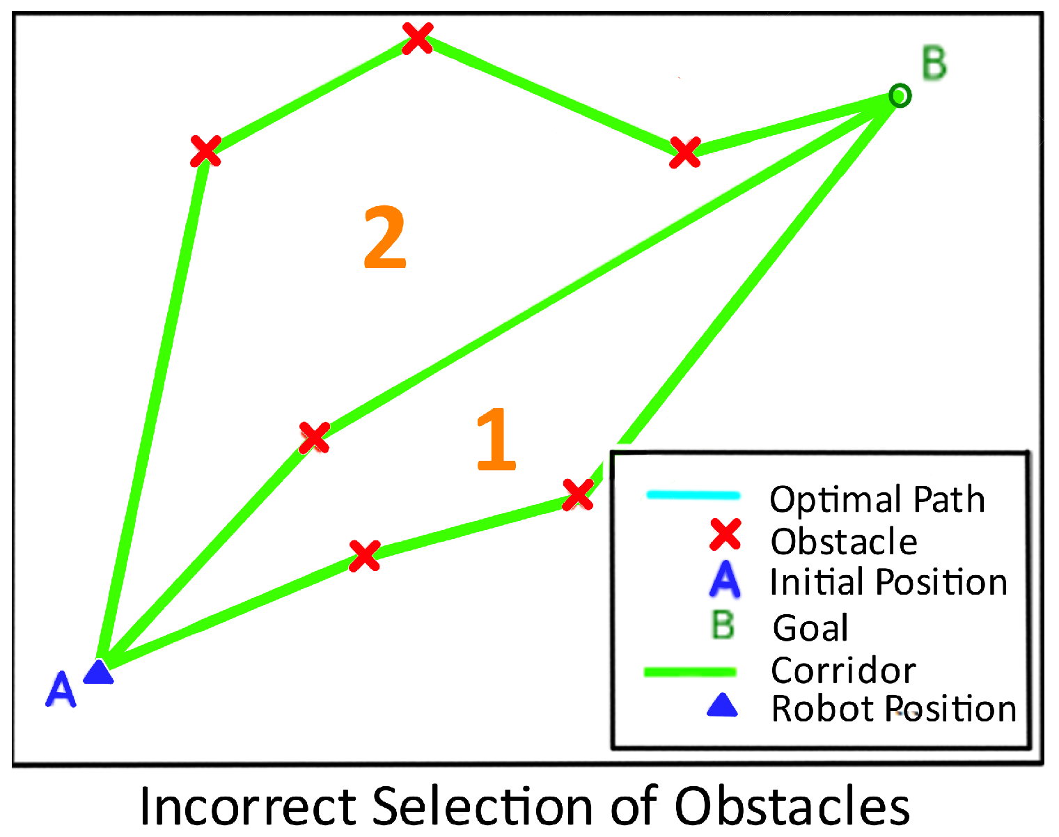
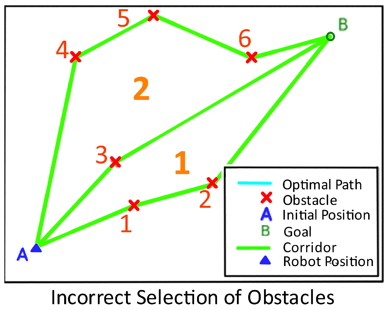
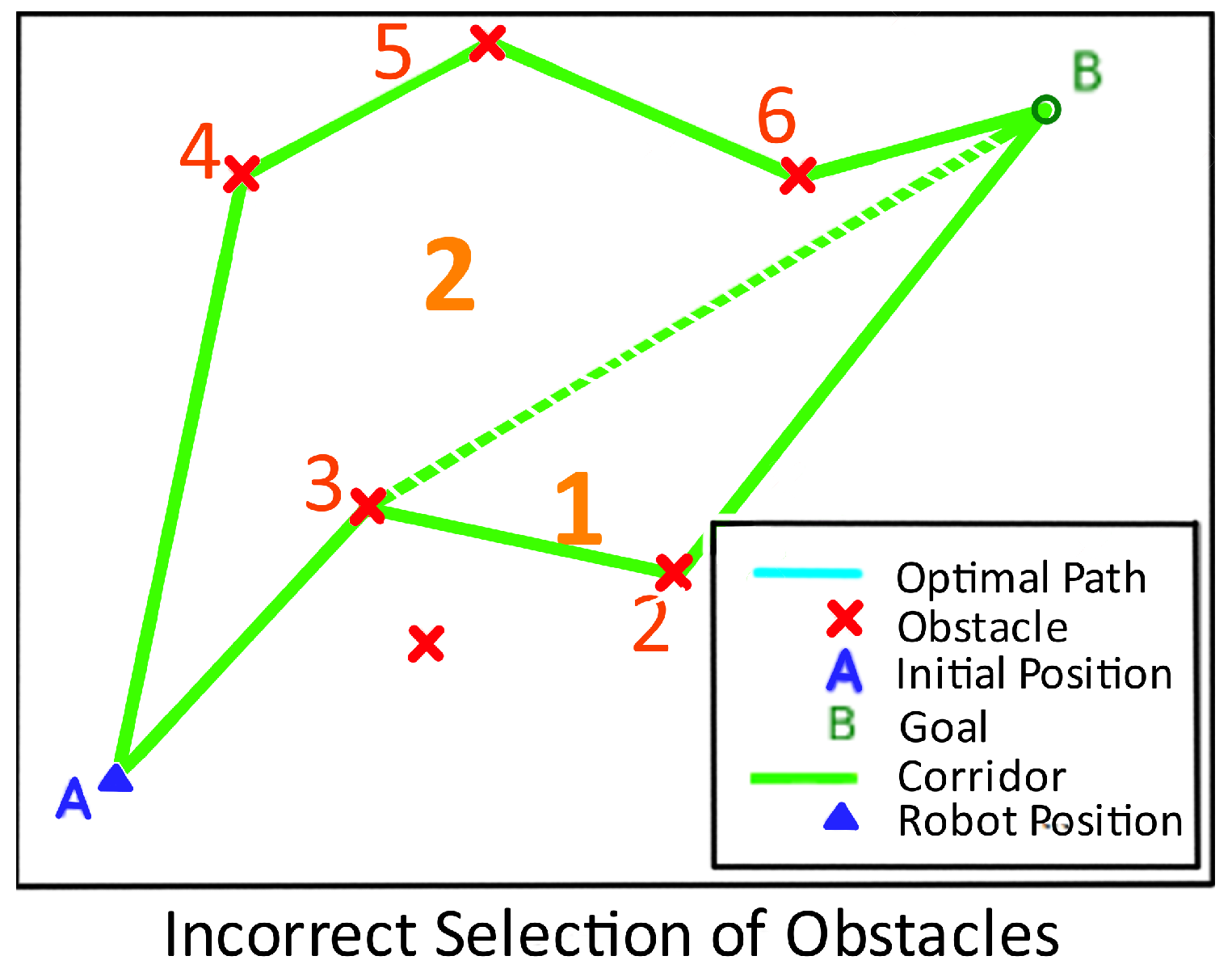
• The algorithm will consider only the obstacles whose distance to the optimal path at any time is lower than 2 m.
• The obstacles closest to the robot’s current position are selected only if their direction vector intersects the robot’s direction vector. In other words, when the closest points pose no collision risk, it is considered that the robot has already surpassed them.

The obstacles must be minimal to prevent situations like the one presented in Figure 4.

Including unnecessary waypoints affects the selection of the optimal corridor because the resulting corridor contains obstacles inside it, as can be seen in Figure 4. The authors’ solution is to detect whether there are obstacles (red crosses) inside the green polygon with vertices A, 1, 2, B, 6, 5, 4. If such points are detected, they need to be removed. The authors numbered the obstacles inside Figure 5.

The figure above showcases that obstacle 3 is inside the selection of points. To transform it into a boundary point, we need to remove one of the closest points and recheck whether point 3 it has become a boundary point.

E.g., after removing the obstacle denoted with 1, the corridors denoted with orange 1 and 2 become parts of a singular corridor, meaning that the robot will pass through both of them, as shown below in Figure 6.

The authors mention that there are cases when it is not sufficient to remove one point, but the solution is simple. If no point suffices, selections of 2 points are tried out. If no combination of 2 points suffice, combinations of 3 points are tried out, etc.

The final step before substituting the obstacles’ positions as waypoints in the classical Bézier curve formula is sorting these points. The algorithm accomplishes this by iterating the points along the optimal path and adding the obstacle closest to the current point to the sorted list.

Figure 7 showcases the adapted Bézier curves algorithm’s steps. In the legend, the blue triangle denotes the robot’s position, the green circle denotes the goal’s position, A and B are the initial and the end position for the robot, the red squares denote the dynamic obstacles. For Figure 7 b-d, the green lines denote the border of the followed corridor and the cyan lines denote the absolute optimal path. Inside Figure 7d, the cyan curve denotes the optimal path generated by the authors’ algorithm.

Figure 7a shows the initial setup of the dynamic environment.

Figure 7b shows the first step: search of the absolute optimal path.

Figure 7c shows the second step: selection of an optimal corridor from point A to point B.

Figure 7d shows the third step: computing the planned path (cyan curve) which will be used by the robot to traverse the dynamic environment.

For obtaining the cyan path from Figure 7d, the algorithm iterates through the next steps:

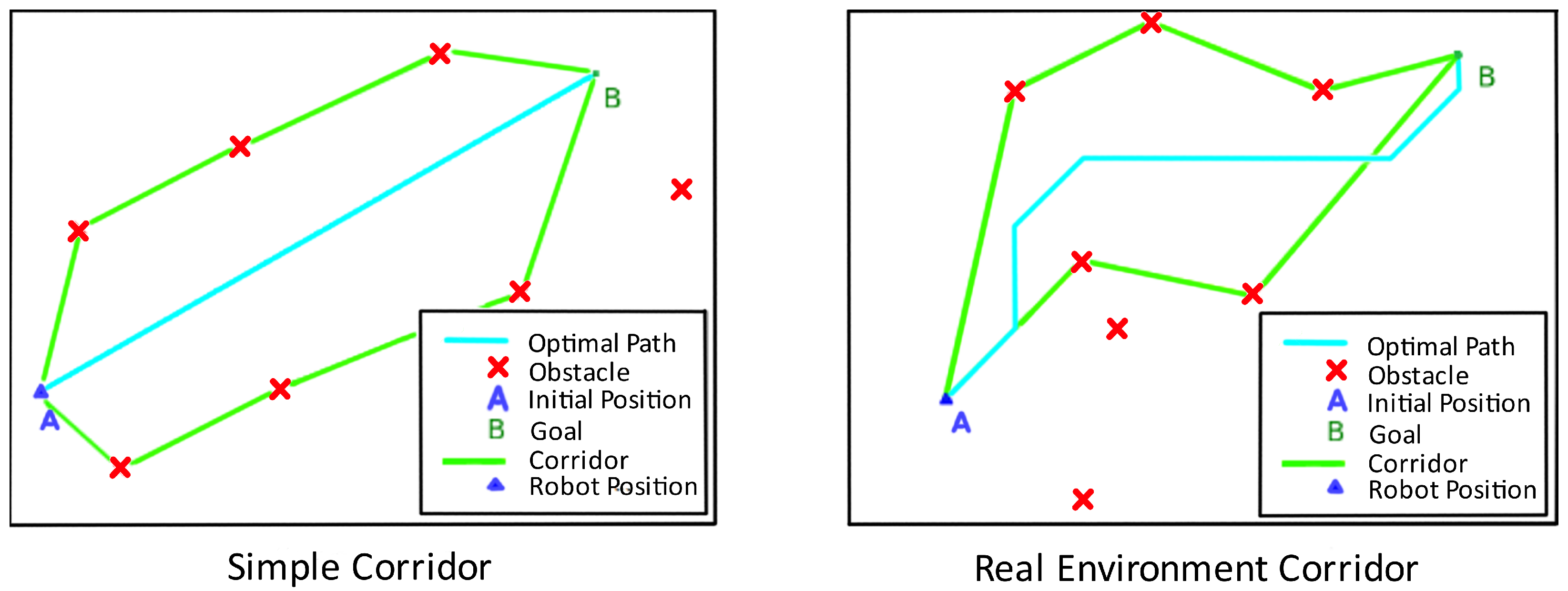
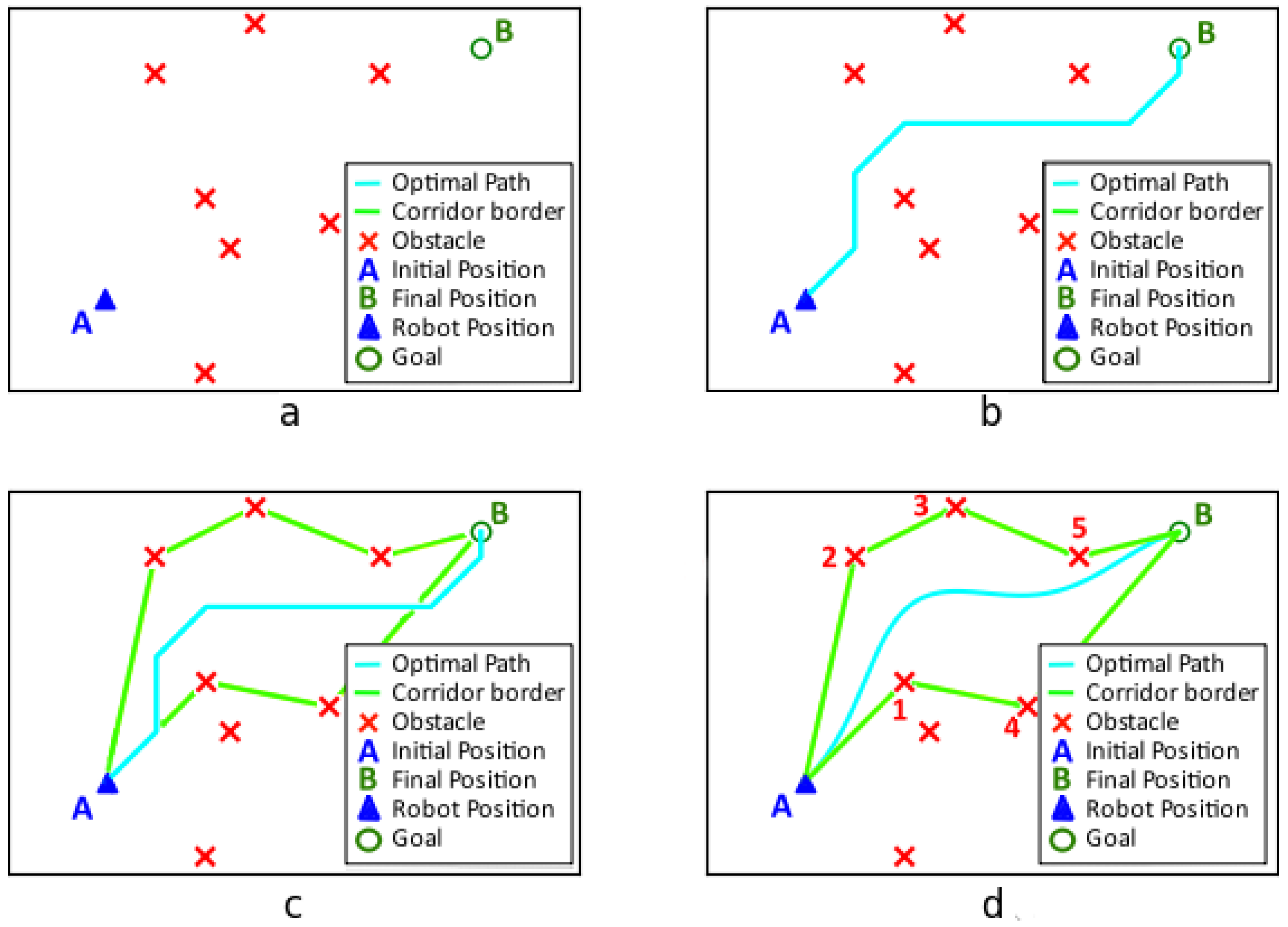
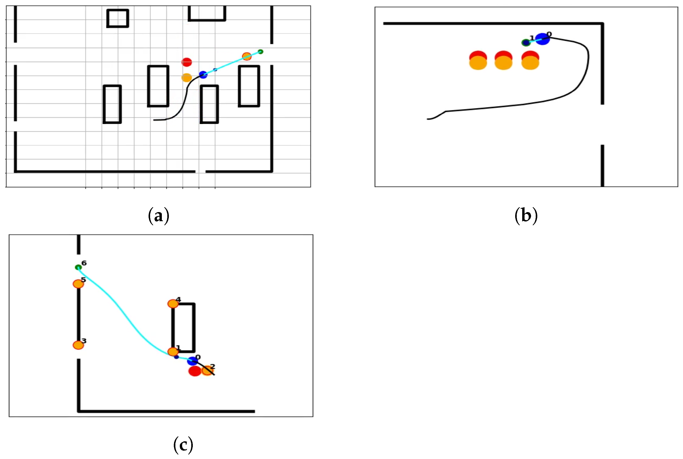
• The algorithm uses a grid-based algorithm such as D* to compute a path of optimal distance (Figure 7b);
• For the chosen path, the algorithm selects a set of obstacles that are the closest to the optimal path and represent the boundaries for the optimal corridor, Figure 7c;
• The points are ordered by the time when the robot will reach the closest position to each one of the points, as can be seen in Figure 7d;
• The algorithm generates a Bézier curve. This curve represents the planned path, as is shown in Figure 7d.

In practice, mobile robots are different in their design. They vary in speed, navigation space, gauge, capacity to turn in different directions in a unit of time, and capacity to accelerate and decelerate. Under such circumstances, the authors identified collisions between the robot and obstacles while testing the adapted Bézier curve algorithm presented in this section.

The authors developed a series of experiments in which the robot collided with the obstacles using the classical Bézier curve model. They represent the space of investigation for an improved algorithm. The complete collisions grouped by the stage where they took place are accessible in Appendix A.

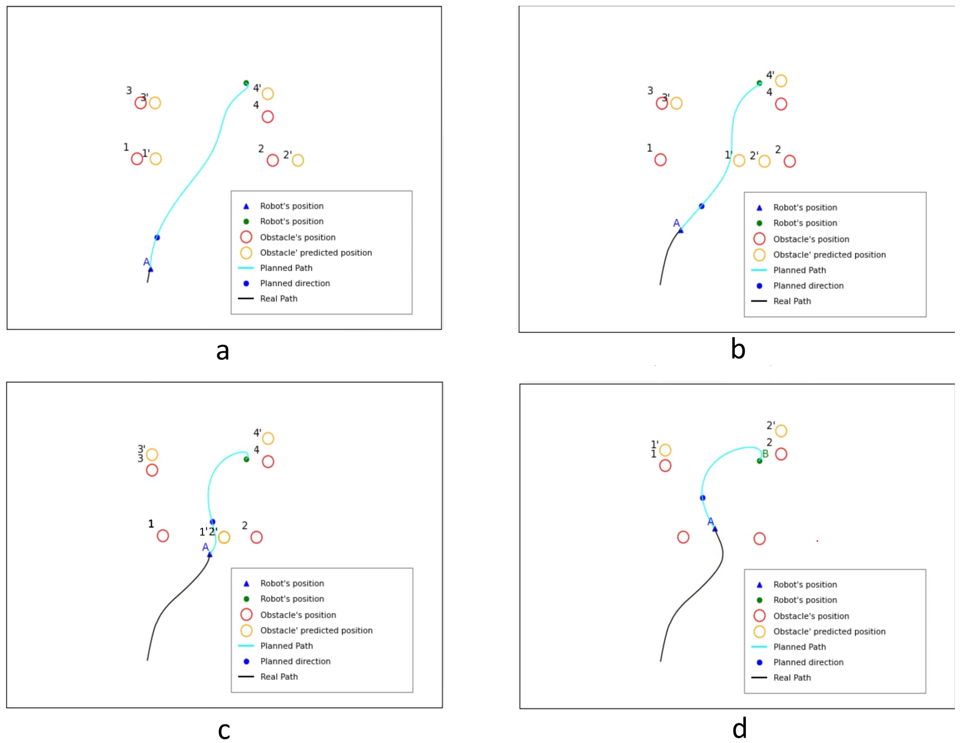
5. Improved Bézier Curve Model for Collision Avoidance

The nine stages indicate, employing simulations in Gazebo, a multitude of collisions. These simulations were calibrated for a mobile robot that used the standard TEB planner from ROS. Therefore, an improved version of the classical algorithm is proposed to face a highly dynamic environment. Some of these simulations were recorded and can be found in Appendix A. Enhancements of the algorithm refer to two extra features:

• Instead of using the obstacles’ current position, the algorithm predicts the obstacles’ position as waypoints by delaying the position by two seconds.
• A new way of path planning when the distance to the closest two obstacles is critical.

The features above are used simultaneously in the algorithm, but the best results are due to the second enhancement, as can be observed in the simulation, whose key moments are captured in Figure 8.

At the start, the robot planner generates a path from A to B (the cyan line in Figure 8a). The cyan line represents the global planner route relative to what the robot perceives at the start moment; as the robot has a scan radius and advances toward the target, the path changes (see the cyan line in Figure 8b, right-side image).

Figure 8a through Figure 8d present how the enhancements action while the robot traverses the dynamic environment. Figure 8a present how the algorithm predicts the position of the obstacles, orders them as notes in the previous section, and creates the smooth path. Figure 8b presents that when the robot is closer to obstacles, the two closest predictions (orange circles denoted 1’ and 2’) are gradually positioned such as the robot passes uniformly (at equal distances) between obstacle 1 and obstacle 2. Figure 8c also showcases the movements of the two closest obstacles. Figure 8d showcases how the closest obstacles are not taken into account after the robot successfully surpasses the obstacles’ direction of deplasation.

As shown in Figure 8, the predicted positions are represented as orange circles and labeled according to the predicted obstacles. If the obstacle is labeled as 1, the prediction will be labeled as 1’. For this experiment, the predictions are computed using their current speed, direction, and a constant time of 3 s.

The second feature of the improved algorithm includes multiple steps, as highlighted in Figure 8b–d. First, let us note that the waypoints used in computing the cyan-colored Bézier curve are the orange predictions (see Figure 8b). When the robot enters the zone preceding the most critical area, the closest waypoint gradually moves toward the second closest waypoint until it perfectly overlays it. The superposition happens when the robot enters the critical area. As a result, the robot’s direction tilts toward the second nearest point.

As shown in Figure 8c, after the robot enters the critical zone, the two overlaid waypoints will gradually move from the closest obstacle’s prediction to the second closest obstacle’s prediction. After the robot surpasses the obstacles, precisely at the moment it is closest to the two superpositioned predicted obstacles, the far two waypoints are eliminated. As shown in Figure 8d, the path remains smooth when using this strategy.

The area preceding the critical zone and the critical zone were delimited using simple rules: whether the distance from the robot to the closest waypoint is less than or equal to 6, respectively, 4 m.

When running the enhanced algorithm, the robot passes between the two closest obstacles by moving toward the second closest obstacle. On the final route, the robot keeps the obstacles at an equal distance. Informally, the robot moves through the middle of the corridor. The link to the recording of the experiment is available in Appendix A.

The Collision Prevention of the Improved Bézier Curve Model

Figure 9 lists screen captures of running the proposed algorithm, and the full recordings are available in Appendix A.

The collision prevention previously illustrated in Figure 8 does not suffice in resolving all collisions, because it provides no option of choosing between stopping the guided robot or detouring dangerous obstacles. The authors developed resolutions for the cases from Figure 9.

The strategies used for cases (a) through (c) also make use of adapting the waypoints but use more conditional cases. Cases (b) and (c) illustrate the conditions. For case (c), the space between the red mobile obstacle and the black shelf was detected as large enough to pass between them, whereas for case (b), the initial trajectory was colliding with the obstacles, so the guided robots stopped for two seconds, after which they look for a detour by using the right-side wall as waypoints.

When a mobile obstacle frontally approaches, the guided robot uses waypoints around the fixed corridor to either accelerate toward and exit or place itself beside one of the fixed corridor sides. For case (a), the robot’s speed was high enough to exit the corridor before the predicted point; therefore, there was no need to stop beside the shelf.

6. Discussion

The discussions from this section are grouped into two parts: the comparative analysis with peer models and the algorithm’s performance.

A peer comparison is a complex issue as long as access to information from other researchers is needed. Tests were conducted with our solution considering a much more complex navigation environment than the cases exemplified in the research cited in Section 2. In addition, we have considered the robot’s navigation algorithm’s physical parameters. From a technical point of view, the enhanced algorithm proposed in this paper proves to be highly agile, with issues that were not considered in the previous research.

In terms of the performance, the proposed navigation model resulted from a systematic deployment of performance indicators. The tests indicate that the targets related to the performance indicators were met without hitting obstacles.

7. Conclusions

The autonomous navigation of mobile robots is a growing interest for researchers and practitioners, especially with the development of industry 4.0 and autonomously driven vehicles. If vehicles come up with a single type of mechanical architecture of the rolling platform, mobile robots are designed with various kinds of rolling architectures. This introduces an additional noise factor concerning the agility of navigation because the construction of the rolling platform strongly influences the performance of the navigation algorithms. In addition, mobile robots operate in indoor spaces too, where the navigation rules are not established. In these environments, there are small spaces for maneuvering, mobile obstacles move in unexpected directions and at incredible speeds, the density of obstacles is random, and the robot’s tasks are diverse.

The test conducted with the TEB planner used by mobile robots driven by the ROS navigation algorithm generates an undesired behavior when the obstacles are dense and the entropy in the environment is high. This behavior means intermittent turns to the left and to the right around a central point of the robot without moving until the algorithm finds a moment of opportunity to select a specific direction of movement. If the dynamics in the environment are high, this behavior repeats again and again. This is not a natural movement of a mobile object (e.g., a person) in an indoor space. In addition, even in this behavioral mode, collisions cannot be avoided for some critical cases (e.g., denser mobile obstacles and higher speeds of the mobile obstacles).

In this research, adapted Bézier curves have been proposed in an attempt to improve the navigation algorithm of a mobile robot (with the physical parameters included in the simulation) in a highly dynamic environment with space constraints for maneuvering. The tests indicate that even if classical Bézier curves bring improvements in the navigation algorithm, if the environment becomes too dense and too dynamic, collisions can happen, except when the robot moves very slowly (which is not necessarily aligned with the performance expectations). However, paths become smoother, and more than this, the algorithm cancels the undesired left–right turns around a point of the robot while deciding what direction to follow. The algorithm is further improved to avoid collisions by introducing features that increase the robot’s agility. They anticipate movements in the navigation space and act accordingly to avoid collisions.

There are still limitations in our research. We did not yet test a wider variety of mobile robots with various gauges and mechanical architectures to argue that the algorithm is robust to any robot structure. Moreover, navigation is not only about movement with a certain speed and obstacle avoidance.

References

1. Abdel-Aziz, H.; Zanaty, E.; Ali, H.A.; Saad, M.K. Generating Bézier curves for medical image reconstruction. Results Phys. 2021, 23, 103996. [Google Scholar] [CrossRef]
2. Bugdol, M.; Juszczyk, J. Parametric curves in liver deformation for laparoscopic purposes. In Information Technologies in Biomedicine; Springer: Berlin/Heidelberg, Germany, 2010; pp. 183–190. [Google Scholar]
3. Alsmadi, M. Facial recognition under expression variations. Int. Arab J. Inf. Technol. 2016, 13, 133–141. [Google Scholar]
4. Cinque, L.; Levialdi, S.; Malizia, A. Shape description using cubic polynomial Bezier curves. Pattern Recognit. Lett. 1998, 19, 821–828. [Google Scholar] [CrossRef]
5. Sederberg, T. Computer Aided Geometric Design; CAGD Course Notes; Brigham Young University Press: Provo, UH, USA, 2012. [Google Scholar]
6. Li, H.; Luo, Y.; Wu, J. Collision-free path planning for intelligent vehicles based on Bézier curve. IEEE Access 2019, 7, 123334–123340. [Google Scholar] [CrossRef]
7. Li, H.; Luo, J.; Yan, S.; Zhu, M.; Hu, Q.; Liu, Z. Research on parking control of bus based on improved pure pursuit algorithms. In Proceedings of the 2019 18th International Symposium on Distributed Computing and Applications for Business Engineering and Science (DCABES), Wuhan, China, 8–10 November 2019; pp. 21–26. [Google Scholar]
8. Liang, Z.; Zheng, G.; Li, J. Automatic parking path optimization based on bezier curve fitting. In Proceedings of the 2012 IEEE International Conference on Automation and Logistics, Zhengzhou, China, 15–17 August 2012; pp. 583–587. [Google Scholar]
9. Xu, L.; Cao, M.; Song, B. A new approach to smooth path planning of mobile robot based on quartic Bezier transition curve and improved PSO algorithm. Neurocomputing 2022, 473, 98–106. [Google Scholar] [CrossRef]
10. Manyam, S.G.; Casbeer, D.W.; Weintraub, I.E.; Taylor, C. Trajectory Optimization For Rendezvous Planning Using Quadratic Bézier Curves. In Proceedings of the 2021 IEEE/RSJ International Conference on Intelligent Robots and Systems (IROS), Prague, Czech Republic, 27 September–1 October 2021; pp. 1405–1412. [Google Scholar]
11. Maqsood, S.; Abbas, M.; Miura, K.T.; Majeed, A.; Iqbal, A. Geometric modeling and applications of generalized blended trigonometric Bézier curves with shape parameters. Adv. Differ. Equ. 2020, 2020, 1–18. [Google Scholar] [CrossRef]
12. BiBi, S.; Abbas, M.; Misro, M.Y.; Hu, G. A novel approach of hybrid trigonometric Bézier curve to the modeling of symmetric revolutionary curves and symmetric rotation surfaces. IEEE Access 2019, 7, 165779–165792. [Google Scholar] [CrossRef]
13. Gim, S.; Adouane, L.; Lee, S.; Derutin, J.P. Clothoids composition method for smooth path generation of car-like vehicle navigation. J. Intell. Robot. Syst. 2017, 88, 129–146. [Google Scholar] [CrossRef] [Green Version]
14. Benko Loknar, M.; Blažič, S.; Klančar, G. Minimum-time velocity profile planning for planar motion considering velocity, acceleration and jerk constraints. Int. J. Control 2021, 94, 1–15. [Google Scholar] [CrossRef]
15. Zdešar, A.; Škrjanc, I. Optimum velocity profile of multiple Bernstein-Bézier curves subject to constraints for mobile robots. ACM Trans. Intell. Syst. Technol. 2018, 9, 1–23. [Google Scholar] [CrossRef]
16. Zhang, T.; Mo, H. Reinforcement learning for robot research: A comprehensive review and open issues. Int. J. Adv. Robot. Syst. 2021, 18, 17298814211007305. [Google Scholar] [CrossRef]
17. Klančar, G.; Seder, M. Coordinated Multi-Robotic Vehicles Navigation and Control in Shop Floor Automation. Sensors 2022, 22, 1455. [Google Scholar] [CrossRef]
18. Sánchez-Ibáñez, J.R.; Pérez-del Pulgar, C.J.; García-Cerezo, A. Path Planning for Autonomous Mobile Robots: A Review. Sensors 2021, 21, 7898. [Google Scholar] [CrossRef] [PubMed]
19. Klančar, G.; Seder, M.; Blažič, S.; Škrjanc, I.; Petrović, I. Drivable Path Planning Using Hybrid Search Algorithm Based on E* and Bernstein–Bézier Motion Primitives. IEEE Trans. Syst. Man Cybern. Syst. 2019, 51, 4868–4882. [Google Scholar] [CrossRef]
20. Casselman, B. From Bézier to Bernstein. In Feature Column from American Mathematical Society; AMS: Providence, RI, USA, 2008. [Google Scholar]
21. Bézier, P.E. Example of an existing system in the motor industry: The Unisurf system. Proc. R. Soc. Lond. Math. Phys. Sci. 1971, 321, 207–218. [Google Scholar]
22. Rubio, F.; Valero, F.; Llopis-Albert, C. A review of mobile robots: Concepts, methods, theoretical framework, and applications. Int. J. Adv. Robot. Syst. 2019, 16, 1729881419839596. [Google Scholar] [CrossRef] [Green Version]
23. González, D.; Pérez, J.; Milanés, V.; Nashashibi, F. A review of motion planning techniques for automated vehicles. IEEE Trans. Intell. Transp. Syst. 2015, 17, 1135–1145. [Google Scholar] [CrossRef]
24. Connors, J.; Elkaim, G. Manipulating B-Spline based paths for obstacle avoidance in autonomous ground vehicles. In Proceedings of the 2007 National Technical Meeting of The Institute of Navigation, Cambridge, MA, USA, 23–25 April 2007; pp. 1081–1088. [Google Scholar]
25. Vickers, N.J. Animal communication: When i’m calling you, will you answer too? Curr. Biol. 2017, 27, R713–R715. [Google Scholar] [CrossRef]
26. Raheem, F.A.; Abdulkareem, M.I. Development of a* algorithm for robot path planning based on modified probabilistic roadmap and artificial potential field. J. Eng. Sci. Technol. 2020, 15, 3034–3054. [Google Scholar]
27. Hart, P.E.; Nilsson, N.J.; Raphael, B. A formal basis for the heuristic determination of minimum cost paths. IEEE Trans. Syst. Sci. Cybern. 1968, 4, 100–107. [Google Scholar] [CrossRef]
28. Raheem, F.A.; Hameed, U.I. Path planning algorithm using D* heuristic method based on PSO in dynamic environment. Am. Acad. Sci. Res. J. Eng. Technol. Sci. 2018, 49, 257–271. [Google Scholar]
29. Lee, C.Y. An algorithm for path connections and its applications. IRE Trans. Electron. Comput. 1961, 3, 346–365. [Google Scholar] [CrossRef] [Green Version]
30. Blažič, S.; Klančar, G. Effective Parametrization of Low Order Bézier Motion Primitives for Continuous-Curvature Path-Planning Applications. Electronics 2022, 11, 1709. [Google Scholar] [CrossRef]
31. Duraklı, Z.; Nabiyev, V. A new approach based on Bezier curves to solve path planning problems for mobile robots. J. Comput. Sci. 2022, 58, 101540. [Google Scholar] [CrossRef]
32. Li, F.F.; Du, Y.; Jia, K.J. Path planning and smoothing of mobile robot based on improved artificial fish swarm algorithm. Sci. Rep. 2022, 12, 659. [Google Scholar] [CrossRef]
33. Song, B.; Wang, Z.; Zou, L. An improved PSO algorithm for smooth path planning of mobile robots using continuous high-degree Bezier curve. Appl. Soft Comput. 2021, 100, 106960. [Google Scholar] [CrossRef]
34. Tharwat, A.; Elhoseny, M.; Hassanien, A.E.; Gabel, T.; Kumar, A. Intelligent Bézier curve-based path planning model using Chaotic Particle Swarm Optimization algorithm. Clust. Comput. 2019, 22, 4745–4766. [Google Scholar] [CrossRef]
35. Rösmann, C.; Feiten, W.; Wösch, T.; Hoffmann, F.; Bertram, T. Efficient trajectory optimization using a sparse model. In Proceedings of the 2013 European Conference on Mobile Robots, Barcelona, Spain, 25–27 September 2013; pp. 138–143. [Google Scholar]
36. Rösmann, C.; Hoffmann, F.; Bertram, T. Kinodynamic trajectory optimization and control for car-like robots. In Proceedings of the 2017 IEEE/RSJ International Conference on Intelligent Robots and Systems (IROS), Vancouver, BC, Canada, 24–28 September 2017; pp. 5681–5686. [Google Scholar]
37. Quigley, M.; Conley, K.; Gerkey, B.; Faust, J.; Foote, T.; Leibs, J.; Wheeler, R.; Ng, A.Y. ROS: An open-source Robot Operating System. In Proceedings of the ICRA Workshop on Open Source Software, Kobe, Japan, 12–17 May 2009; Volume 3, p. 5. [Google Scholar]
38. Quinlan, S.; Khatib, O. Elastic bands: Connecting path planning and control. In Proceedings of the 1993 IEEE International Conference on Robotics and Automation, Atlanta, GA, USA, 2–6 May 1993; pp. 802–807. [Google Scholar]
39. Wu, J.; Ma, X.; Peng, T.; Wang, H. An Improved Timed Elastic Band (TEB) Algorithm of Autonomous Ground Vehicle (AGV) in Complex Environment. Sensors 2021, 21, 8312. [Google Scholar] [CrossRef]
40. Chen, W.; Liu, J.; Tang, Y.; Ge, H. Automatic Spray Trajectory Optimization on Bézier Surface. Electronics 2019, 8, 168. [Google Scholar] [CrossRef] [Green Version]
41. Zhu, X.; Wang, M.; Ruan, X.; Chen, L.; Ji, T.; Liu, X. Adaptive Motion Skill Learning of Quadruped Robot on Slopes Based on Augmented Random Search Algorithm. Electronics 2022, 11, 842. [Google Scholar] [CrossRef]
42. Choi, J.W.; Curry, R.; Elkaim, G. Path planning based on bézier curve for autonomous ground vehicles. In Proceedings of the Advances in Electrical and Electronics Engineering-IAENG Special Edition of the World Congress on Engineering and Computer Science 2008, Sozopol, Bulgaria, 11–14 September 2008; pp. 158–166. [Google Scholar]
43. Preparata, F.P.; Shamos, M.I. Computational Geometry: An Introduction; Springer Science & Business Media: Berlin/Heidelberg, Germany, 2012. [Google Scholar]
44. Koenig, N.; Howard, A. Design and use paradigms for gazebo, an open-source multi-robot simulator. In Proceedings of the 2004 IEEE/RSJ International Conference on Intelligent Robots and Systems (IROS)(IEEE Cat. No. 04CH37566), Sendai, Japan, 28 September–2 October 2004; Volume 3, pp. 2149–2154. [Google Scholar]
45. Sokolov, M.; Gabdullin, A.; Afanasyev, I.; Lavrenov, R.; Magid, E. 3D modelling and simulation of a crawler robot in ROS/Gazebo. In Proceedings of the 4th International Conference on Control, Mechatronics and Automation, Barcelona, Spain, 7–11 December 2016; pp. 61–65. [Google Scholar] [CrossRef]
46. Mengacci, R.; Zambella, G.; Grioli, G.; Caporale, D.; Catalano, M.G.; Bicchi, A. An Open-Source ROS-Gazebo Toolbox for Simulating Robots With Compliant Actuators. Front. Robot. AI 2021, 246. [Google Scholar] [CrossRef] [PubMed]
47. Gelperin, D. On the optimality of A*. Artif. Intell. 1977, 8, 69–76. [Google Scholar] [CrossRef]
48. Lu, D.V.; Hershberger, D.; Smart, W.D. Layered costmaps for context-sensitive navigation. In Proceedings of the 2014 IEEE/RSJ International Conference on Intelligent Robots and Systems, Chicago, IL, USA, 14–18 September 2014; pp. 709–715. [Google Scholar]
49. Thrun, S. Simultaneous Localization and Mapping. In Robotics and Cognitive Approaches to Spatial Mapping; Jefferies, M.E., Yeap, W.K., Eds.; Springer: Berlin/Heidelberg, Germany, 2008; pp. 13–41. [Google Scholar] [CrossRef]
50. Kohlbrecher, S.; Von Stryk, O.; Meyer, J.; Klingauf, U. A flexible and scalable SLAM system with full 3D motion estimation. In Proceedings of the 2011 IEEE International Symposium on Safety, Security, and Rescue Robotics, Kyoto, Japan, 1–5 November 2011; pp. 155–160. [Google Scholar]
51. Overmars, M.; Karamouzas, I.; Geraerts, R. Flexible path planning using corridor maps. In Proceedings of the European Symposium on Algorithms, Karlsruhe, Germany, 15–17 September 2008; pp. 1–12. [Google Scholar]
Figure 1. The nine stages selected using Table 1 and Table 3. The captures are taken from Gazebo. The white and colored objects represent mobile and fixed obstacles. The full description of the nine stages can be found above, listed from (a) to (i). (a) Stage 1; (b) Stage 2; (c) Stage 3; (d) Stage 4; (e) Stage 5; (f) Stage 6; (g) Stage 7; (h) Stage 8; (i) Stage 9.
Electronics 11 03568 g001
Figure 2. Illustrative examples of weaknesses detected while running the classical TEB planner inside the 9 stages. The blue rectangle represents the robot, red arrow represents the path, the grey shadow represents the obstacles, red arcs represent the contours of the obstacles detected by the ROS packages. (a) Stage 1, the planner cannot avoid collision when passing through narrow corridors; (b) Stage 2, planner passed through obstacle instead of slowing or detouring; (c) Stage 3, planner crosses the obstacle’s frontal side.
Electronics 11 03568 g002
Figure 3. Examples of corridors.
Electronics 11 03568 g003
Figure 4. Selection of too many obstacles leads to the selection of multiple corridors.
Electronics 11 03568 g004
Figure 5. How to remove extra obstacles from selection.
Electronics 11 03568 g005
Figure 6. How the corridors merge after removal of extra obstacles.
Electronics 11 03568 g006
Figure 7. Steps of the Adapted Bézier Curve Algorithm.
Electronics 11 03568 g007
Figure 8. Collision prevention using the improved Bézier curve algorithm.
Electronics 11 03568 g008
Figure 9. How various collisions are prevented using the adapted Bezier curve algorithm from Section 5. (a) Resolving a collision inside a tight, fixed-width corridor; (b) resolving a lateral collision in Stage 9; (c) resolving a frontal collision in Stage 8.
Electronics 11 03568 g009