An Efficient Estimation Method for Dynamic Systems in the Presence of Inaccurate Noise Statistics

Abstract

The uncertainty of noise statistics in dynamic systems is one of the most important issues in engineering applications, and significantly affects the performance of state estimation. The optimal Bayesian Kalman filter (OBKF) is an important approach to solve this problem, as it is optimal over the posterior distribution of unknown noise parameters. However, it is not suitable for online estimation because the posterior distribution of unknown noise parameters at each time is derived from its prior distribution by incorporating the whole measurement sequence, which is computationally expensive. Additionally, when the system is subjected to large disturbances, its response is slow and the estimation accuracy deteriorates. To solve the problem, we improve the OBKF mainly in two aspects. The first is the calculation of the posterior distribution of unknown noise parameters. We derive it from the posterior distribution at a previous time rather than the prior distribution at the initial time. Instead of the whole measurement sequence, only the nearest fixed number of measurements are used to update the posterior distribution of unknown noise parameters. Using the sliding window technique reduces the computational complexity of the OBKF and enhances its robustness to jump noise. The second aspect is the estimation of unknown noise parameters. The posterior distribution of an unknown noise parameter is represented by a large number of samples by the Markov chain Monte Carlo approach. In the OBKF, all samples are equivalent and the noise parameter is estimated by averaging the samples. In our approach, the weights of samples, which are proportional to their likelihood function values, are taken into account to improve the estimation accuracy of the noise parameter. Finally, simulation results show the effectiveness of the proposed method.

1. Introduction

State estimation is one of the most important issues in many engineering applications, such as energy internet, navigation, control systems, and so on [1,2,3,4]. These systems are, in essence, dynamic systems, which are usually described by the well-known state-space models. The state estimation problem can be briefly formulated as follows: given the mathematical model of a dynamic system, it is desirable to estimate the time-varying state from noise-contaminated measurements [5,6]. For linear dynamic systems, the state estimation problem can be solved by the classical Kalman filter (KF) [7], which is an optimal filter in minimum mean square-root error (MMSE). For nonlinear cases, several variants of the KF have been developed, such as the extended KF, the unscented KF, and the cubature KF, to name but a few [8]. The KF and its variants have simple forms, and have been widely used in many real-world applications [1,9].

The KF, in general, performs well for dynamic systems with known noise statistics. However, exact knowledge of the noise statistics of the underlying stochastic processes may not be available in practice. For example, the dynamic system may be subjected to potential non-stationary noise; that is, the system noise may be slowly varying [10]. Another typical scene is that the system noise may jump as the environment changes [11]. When the exact noise statistics are unknown, the performance of the KF may seriously deteriorate. The main reason for this problem is that the standard KF is derived under the MMSE criterion, which requires accurate information of the noise statistics of the dynamic system.

In order to solve the problem of uncertain noise statistics, a large number of robust KFs have been proposed [12,13]. A typical solution is to design an adaptive KF, in which the noise statistics and the state are jointly estimated [11,14]. However, the joint distribution of the state and noise parameters is analytically difficult, and a variational Bayesian technique is usually used to compute the joint distribution. This requires high computational effort, as a fixed-point iteration is involved to compute the separable variational approximation, which limits its practical application. Another solution is the minimax linear state estimation approach, in which the minimum-error upper bound of all possible noise covariances is considered [15]. However, the standard KF is derived under the MMSE criterion, in which accurate noise covariances are needed. Therefore, inaccurate noise covariance may lead to poor performance of the KF and unreliable state estimation.

Recently, an intrinsic Bayesian robust Kalman filter (IBRKF) [16] and an optimal Bayesian Kalman filter (OBKF) [17] were developed from the perspective of minimizing the mean square error. They are optimal with respect to the prior and the posterior distributions of unknown noise statistical parameters, respectively. In the OBKF, a factor graph approach [18] is employed to characterize the relationship between the prior distribution and the posterior distribution of unknown noise statistical parameters, formulated as a message-passing process [19]. However, the OBKF is not suitable for online estimation, since the likelihood function of unknown noise statistical parameters with respected to the whole measurement sequence needs to be calculated at each step, and the computational effort of the likelihood function dramatically increases over time. In addition, when the system is subjected to large disturbances such as jump noise, the response of the OBKF is slow and its estimation accuracy deteriorates.

To solve the above problem, an improved OBKF for dynamic systems with inaccurate noise statistics is developed in this paper. A sliding window technique [20] is used to computing the likelihood function of noise statistical parameters, which is formulated as a message-passing process based on a factor graph. Instead of the whole measurement sequence, only a limited number of measurements closest to the current time are used to update the posterior distribution of the noise statistical parameters. This significantly reduces the computational complexity of the algorithm and particularly enhances its robustness to jump noise. The weights of the measurements are taken into account when computing the posterior distribution of unknown noise statistical parameters, which further improves the state estimation accuracy and the parameters of noise statistics. The proposed method has a simple form, which facilitates its application. Finally, the proposed approach is verified by two scenarios of time-invariant and time-varying noise statistics, respectively. Simulation results show that the proposed algorithm significantly improves response time and estimation accuracy.

The rest of the paper is organized as follows. Section 2 is the problem formulation. Section 3 provides an improved optimal Bayesian approach. In Section 4, we validate the proposed algorithm via simulations. Finally, a conclusion is provided in Section 5.

2. Problem Formulation

State estimation problems are usually solved in the framework of the state-space model. In general, it is necessary to extract the exact knowledge of system noise statistics to design an optimal filter. However, in many real-world applications, it is impossible to obtain the accurate information of noise statistical parameters due to limited data, uncertain disturbances, environmental changes, etc. [21,22].

Assuming that the covariance matrices $Q_k$ and $R_k$ of process noise and measurement noise are unknown, they are respectively represented by the parameters ${\theta }_1$ and ${\theta }_2$ as follows:

$$E\left[w_k^{{\theta }_1}{\left(w_k^{{\theta }_1}\right)}^T\right]=Q_k^{{\theta }_1}{\delta }_{kl}$$

(1)

$$E\left[v_k^{{\theta }_2}{\left(v_k^{{\theta }_2}\right)}^T\right]=R_k^{{\theta }_2}{\delta }_{kl}$$

(2)

where $E\left[·\right]$ denotes an expectation operator and ${\left(·\right)}^T$ is a transition operator. Let $\theta =\left[{\theta }_1,{\theta }_2\right]\in \Theta$ be the unknow noise statistical parameters, and its prior distribution is $\pi \left(\theta \right)$. Because parameters ${\theta }_1$ and ${\theta }_2$ are, in general, independent, the linear state-space model can be described as

$$x_{k+1}^{{\theta }_1}=F_k{x}_k^{{\theta }_1}+G_k{w}_k^{{\theta }_1}$$

(3)

$$y_k^{\theta }=H_k{x}_k^{{\theta }_1}+v_k^{{\theta }_2}$$

(4)

From (3) and (4), it can be seen that the state $x_k^{{\theta }_1}$ is only related to the parameter ${\theta }_1$, while the measurement $y_k^{\theta }$ is related to the parameters ${\theta }_1$ and ${\theta }_2$. Let $\pi \left(\theta |y_{0:k}\right)$ denote the posterior distribution of unknown parameter $\theta$, where $y_{0:k}=\left\{y_0^{\theta },\dots ,y_k^{\theta }\right\}$.

An optimal Bayesian Kalman filter (OBKF) [17] is proposed to solve the estimation problem for the dynamic system with unknown noise statistics; it is optimal with respect to the posterior distribution $\pi \left(\theta |y_{0:k}\right)$ of unknown noise statistical parameter $\theta$. The prediction step of the OBKF is the same as that of the KF, and its update step is summarized as follows:

$$e_k^{\theta }=y_k^{\theta }-H_k{\widehat{x}}_k^{\theta }$$

(5)

$$K_k^{\theta }=E_{\theta }\left[P_k^{\theta }|y_{0:k-1}\right]H_k^T{E}_{\theta }^T\left[H_k{P}_k^{\theta }{H}_k^T|y_{0:k-1}+R_k^{{\theta }_2}|y_{0:k}\right]$$

(6)

$${\widehat{x}}_{k+1}^{\theta }=F_k{\widehat{x}}_k^{\theta }+K_k^{\theta }{e}_k^{\theta }$$

(7)

$$E_{\theta }\left[P_k^{\theta }|y_{0:k}\right]=F_k\left(I-K_k^{\theta }{H}_k\right)E_{\theta }\left[P_k^{\theta }|y_{0:k-1}\right]F_k^T+G_k{E}_{\theta }\left[Q_k^{{\theta }_1}|y_{0:k}\right]G_k^T$$

(8)

where $e_k^{\theta }$ is the innovation, $K_k^{\theta }$ is the gain matrix, I is the identity matrix with an appropriate dimension, ${\widehat{x}}_k^{\theta }$ is the estimation of the state, and $P_k^{\theta }$ is the corresponding covariance matrix. The OBKF has a similar recursive structure to the standard KF, except that it uses the posterior effective process noise covariance $E_{\theta }\left[Q_k^{{\theta }_1}|y_{0:k}\right]$, the posterior effective measurement noise covariance $E_{\theta }\left[R_k^{{\theta }_2}|y_{0:k}\right]$, and the effective gain matrix $K_k^{\theta }$ to replace the corresponding matrices of $Q_k$, $R_k$, and $K_k$.

The key to implementing the OBKF is to compute posterior effective noise covariance matrices $E_{\theta }\left[Q_k^{{\theta }_1}|y_{0:k}\right]$ and $E_{\theta }^T\left[R_k^{{\theta }_2}|y_{0:k}\right]$, which can then be used to compute the effective gain matrix $K_k^{\theta }$. According to Bayes’ theorem, the posterior distribution of the unknown noise statistical parameters is $\pi \left(\theta |y_{0:k}\right)\propto f\left(y_{0:k}|\theta \right)\pi \left(\theta \right)$, which usually has no analytic solution for most prior distributions. In the OBKF, the Markov chain Monte Carlo (MCMC) approach is firstly used to generate the particles of the posterior distribution of noise statistics; then, the noise covariance matrix is approximated by calculating the mean value of particles. To compute the likelihood function $f\left(y_{0:k}|\theta \right)$, a factor graph approach is employed to formulate the likelihood function as a message-passing process. Although the OBKF has a closed form, it is not suitable for online estimation, since the likelihood function of unknown noise statistical parameters with respect to the whole measurement sequence needs to be calculated at each step. Particularly, the computational effort of the likelihood function dramatically increases over time. In addition, when the system noise jumps due to environmental changes, the response of the OBKF is slow and its estimation accuracy deteriorates.

To address the above problem, an improved OBKF is designed in the next section. It is mainly improved from the following two aspects. The first is the calculation of the posterior distribution of noise parameters. We derive it from the posterior distribution at a previous time rather than its prior distribution at the initial time. Instead of the whole measurement sequence, only the nearest fixed number of measurements are used to update the posterior distribution of unknown noise parameters. By using the sliding window technique, it reduces the computational complexity of the OBKF and enhances its robustness to jump noise. The second is the estimation of unknown noise parameters. The posterior distribution of an unknown noise parameter is represented by a large number of samples by the MCMC approach. In the OBKF, all samples are equivalent, and the noise parameter is estimated by averaging the samples. In our approach, the weights of samples, which are proportional to their likelihood function values, are taken into account to improve the estimation accuracy of the noise parameter.

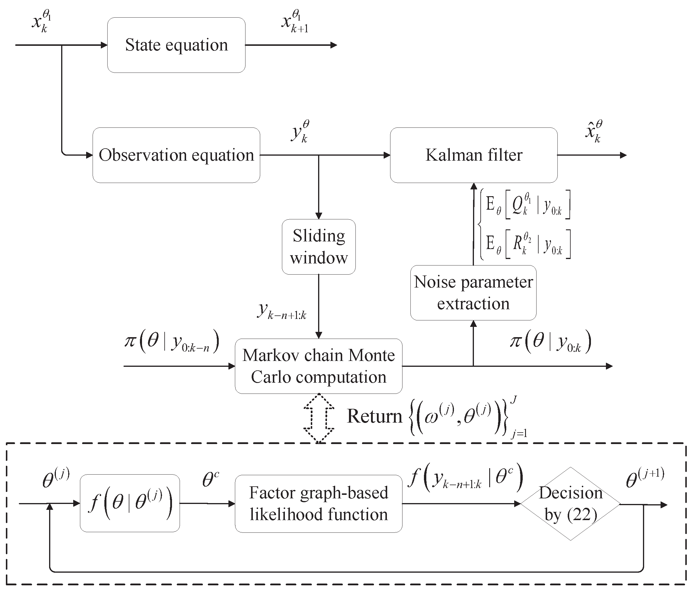
3. Improved Optimal Bayesian Kalman Filter

In this section, an improved optimal Bayesian Kalman filter (IOBKF) is designed to solve the estimation problem for dynamic systems with inaccurate noise statistics. In the traditional OBKF, it is computationally expensive to obtain the posterior distribution of noise statistical parameters. To solve this problem, a sliding window-based approach is proposed to rapidly compute posterior effective noise covariance matrices $E_{\theta }\left[Q_k^{{\theta }_1}|y_{0:k}\right]$ and $E_{\theta }\left[R_k^{{\theta }_2}|y_{0:k}\right]$.

When calculating the posterior distribution $\pi \left(\theta |y_{0:k}\right)$ of unknown noise statistical parameters at time k, the posterior information $\pi \left(\theta |y_{0:l}\right)$ at any previous time $l\le k-1$ is obtained. According to Bayes’ theorem [8], the posterior distribution $\pi \left(\theta |y_{0:k}\right)\propto f\left(y_{0:k}|\theta \right)\pi \left(\theta \right)$ can be rewritten as

$$\pi \left(\theta |y_{0:k}\right)\propto f\left(y_{k-n+1:k}|\theta \right)\pi \left(\theta |y_{0:k-n}\right)$$

(9)

where n is the size of sliding window and is a positive integer, and $f\left(y_{k-n+1:k}|\theta \right)$ is the likelihood function of unknown parameter $\theta$ with respect to the measurements from time $k-n+1$ to time k. Therefore, the posterior distribution $\pi \left(\theta |y_{0:k}\right)$ can be obtained by computing $f\left(y_{k-n+1:k}|\theta \right)$ instead of $f\left(y_{0:k}|\theta \right)$ at each time, which is shown in Figure 1. Only n measurements are involved for computing the new likelihood function $f\left(y_{k-n+1:k}|\theta \right)$, while the whole measurement sequence is used to compute the original likelihood function $f\left(y_{0:k}|\theta \right)$. This can significantly reduce the computational complexity of the algorithm and enhance its robustness to jumping noise.

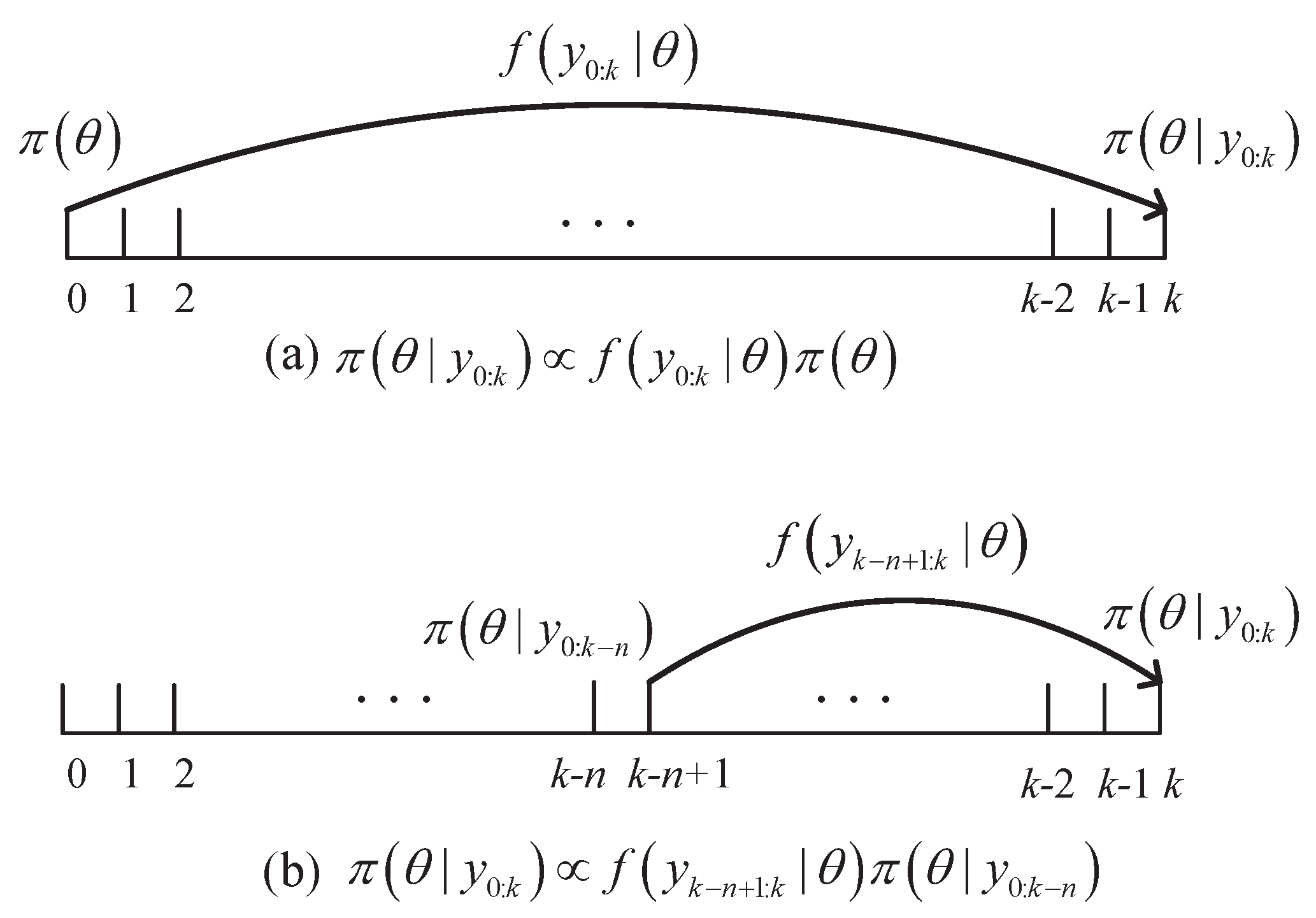
3.1. Calculation of Likelihood Function

We mainly focus on how to calculate the likelihood function $f\left(y_{k-n+1:k}|\theta \right)$ in this section. Inspired by [17], the likelihood function is also formulated as a message-passing process by using a factor graph. Instead of the whole measurement sequence involved in $f\left(y_{0:k}|\theta \right)$, only n measurements are used to compute $f\left(y_{k-n+1:k}|\theta \right)$, since the posterior distribution $\pi \left(\theta |y_{0:k}\right)$ is updated by the prior distribution $\pi \left(\theta |y_{0:k-n}\right)$ in this paper.

In a discrete-time state-space model, according to the properties of a Markov chain, the measurement $y_k$ and the state $x_{k+1}$ are only related to the state $x_k$; i.e.,

$$f\left(y_k|y_{0:k-1},x_{0:k},\theta \right)=f\left(y_k|x_k,\theta \right)=\mathcal{N}\left(y_k;H_k{x}_k,R_k^{{\theta }_2}\right)$$

(10)

$$f\left(x_{k+1}|y_{0:k+1},x_{0:k},\theta \right)=f\left(x_{k+1}|x_k,\theta \right)=\mathcal{N}\left(x_{k+1};F_k{x}_k,{\tilde{Q}}_i^{{\theta }_1}\right)$$

(11)

where ${\tilde{Q}}_i^{{\theta }_1}=G_k{Q}_k^{{\theta }_1}{G}_k^T$, and $\mathcal{N}\left(·;m,P\right)$ denote a Gaussian distribution with mean m and covariance P. To compute the likelihood function $f\left(y_{k-n+1:k}|\theta \right)$, we can formulate it as the marginal distribution of $f\left(y_{k-n+1:k},x_{k-n+1:k}|\theta \right)$ with respect to $x_{k-n+1:k}$, in which the function $f\left(y_{k-n+1:k},x_{k-n+1:k}|\theta \right)$ can be computed by

$$\begin{array}{cc}\hfill & f\left(y_{k-n+1:k}|\theta \right)={\int }_{x_k}\dots {\int }_{x_{k-n+1}}f\left(y_{k-n+1:k},x_{k-n+1:k}|\theta \right)d{x}_{k-n+1}\dots d{x}_k\hfill \\ \hfill & ={\int }_{x_k}\dots {\int }_{x_{k-n+1}}f\left(y_k|x_k,\theta \right)f\left(y_{k-n+1:k-1},x_{k-n+1:k}|\theta \right)d{x}_{k-n+1}\dots d{x}_k\hfill \\ \hfill & ={\int }_{x_k}\dots {\int }_{x_{k-n+1}}f\left(y_k|x_k,\theta \right)f\left(x_k|x_{k-1},\theta \right)f\left(y_{k-n+1:k-1},x_{k-n+1:k-1}|\theta \right)d{x}_{k-n+1}\dots d{x}_k\hfill \\ \hfill & ⋮\hfill \\ \hfill & ={\int }_{x_k}\dots {\int }_{x_{k-n+1}}\prod _{i=k-n+1}^{k}f\left(y_i|x_i,\theta \right)\prod _{i=k-n+2}^{k}f\left(x_i|x_{i-1},\theta \right)f\left(x_{k-n+1}\right)d{x}_{k-n+1}\dots d{x}_k\hfill \end{array}$$

(12)

where the second and third formulas use Markov assumptions (10) and (11), and the distribution $f\left(x_{k-n+1}\right)$ can be replaced by the posterior distribution $f\left(x_{k-n+1}|y_{0:k-n+1}\right)$, which is obtained at time $k-n+1$.

The likelihood function $f\left(y_{k-n+1:k}|\theta \right)$ of the form (12) can be formulated as a message-passing process from time $k-n+1$ to time k based on a factor graph. A factor graph can transform a global function into a product form of local functions. We abbreviate the variable node $x_i$ and factor nodes $f\left(x_i|x_{i-1},\theta \right)$ and $f\left(y_i|x_i,\theta \right)$ as ${\alpha }_i$, ${\beta }_i$, and ${\gamma }_i$, respectively. In a factor graph, the transmitted message contains three components: the scale, mean vector, and covariance matrix of a scaled multivariable Gaussian function [17]. Lemma 1 shows how to transfer a message from ${\beta }_i$ to ${\alpha }_i$.

Lemma 1.

Assuming that a message ${\mu }_{{\beta }_i\to {\alpha }_i}=\left(S_i,M_i,{\Sigma }_i\right)$ transmitted from ${\beta }_i$ to ${\alpha }_i$ is a scaled multivariate Gaussian function $S_i\mathcal{N}\left(x_i;M_i,{\Sigma }_i\right)$, the message ${\mu }_{{\beta }_{i+1}\to {\alpha }_{i+1}}=\left(S_{i+1},M_{i+1},{\Sigma }_{i+1}\right)$ transmitted from ${\beta }_{i+1}$ to ${\alpha }_{i+1}$ is still a scaled multivariate Gaussian function with the form $S_{i+1}\mathcal{N}\left(x_{i+1};M_{i+1},{\Sigma }_{i+1}\right)$, in which the parameters are computed by [17]

$$S_{i+1}=S_i\sqrt{\frac{\left|{\Lambda }_i\right|\left|{\Sigma }_{i+1}\right|}{\left|{\tilde{Q}}_i^{{\theta }_1}\right|\left|{\Sigma }_i\right|}}\mathcal{N}\left(y_i;0,R_i^{{\theta }_1}\right)exp\left(\frac{M_{i+1}^T{\Sigma }_{i+1}^{-1}{M}_{i+1}+W_i^T{\Lambda }_i{W}_i-M_i^T{\Sigma }_i^{-1}{M}_i}{2}\right)$$

(13)

$$M_{i+1}={\Sigma }_{i+1}{\left({\tilde{Q}}_i^{{\theta }_1}\right)}^{-1}{F}_i{\Lambda }_i\left(H_i^T{\left(R_i^{{\theta }_2}\right)}^{-1}{y}_i+{\Sigma }_i^{-1}{M}_i\right)$$

(14)

$${\Sigma }_{i+1}^{-1}={\left({\tilde{Q}}_i^{{\theta }_1}\right)}^{-1}-{\left({\tilde{Q}}_i^{{\theta }_1}\right)}^{-1}{F}_i{\Lambda }_i{F}_i^T{\left({\tilde{Q}}_i^{{\theta }_1}\right)}^{-1}$$

(15)

where

$$W_i=H_i^T{\left(R_i^{{\theta }_2}\right)}^{-1}{y}_i+{\Sigma }_i^{-1}{M}_i$$

(16)

$${\Lambda }_i={\left(F_i^T{\left({\tilde{Q}}_i^{{\theta }_1}\right)}^{-1}{F}_i+H_i^T{\left(R^{{\theta }_2}\right)}^{-1}{H}_i+{\Sigma }_i^{-1}\right)}^{-1}$$

(17)

Using Lemma 1, the likelihood function $f\left(y_{k-n+1:k}|\theta \right)$ can be obtained by iterative operations from time $k-n+1$ to time k; i.e.,

$$\begin{array}{cc}\hfill & f\left(y_{k-n+1:k}|\theta \right)={\int }_{x_k}\mathcal{N}\left(y_k;H_k{x}_k,R_k^{{\theta }_2}\right)\mathcal{N}\left(x_k;M_k,{\Sigma }_k\right)d{x}_k\hfill \\ \hfill & =S_k\sqrt{\frac{\left|{\Delta }_k\right|}{\left|{\Sigma }_k\right|}}\mathcal{N}\left(y_k;0,R_k^{{\theta }_2}\right)exp\left(\frac{1}{2}\left({{\rm Y}}_k^T{\Delta }_k{{\rm Y}}_k-M_k^T{\Sigma }_k^{-1}{M}_k\right)\right)\hfill \end{array}$$

(18)

where

$${\Delta }_k^{-1}=H_k^T{\left(R_k^{{\theta }_2}\right)}^{-1}{H}_k+{\Sigma }_k^{-1}$$

(19)

$${{\rm Y}}_k={\Delta }_k\left(H_k^T{\left(R_k^{{\theta }_2}\right)}^{-1}{y}_k+{\Sigma }_k^{-1}{M}_k\right)$$

(20)

In summary, we can use the factor graph-based message-passing method to calculate the likelihood function $f\left(y_{k-n+1:k}|\theta \right)$ in the form of (18), where the parameters $S_k$, $M_k$, and ${\Sigma }_k$ are calculated from (13)–(15), and the parameters ${\Delta }_k$ and ${{\rm Y}}_k$ are calculated by (19) and (20), respectively.

3.2. Calculation of Posterior Effective Noise Statistics

To compute posterior effective noise covariance matrices $E_{\theta }\left[Q_k^{{\theta }_1}|y_{0:k}\right]$ and $E_{\theta }\left[R_k^{{\theta }_2}|y_{0:k}\right]$, the Metropolis Hastings MCMC method is used to generate the sample set ${\left\{\left({\omega }^{\left(j\right)},{\theta }^{\left(j\right)}\right)\right\}}_{j=1}^J$, where ${\theta }^{\left(j\right)}$ represents the $j\mathrm{th}$ MCMC sample, ${\omega }^{\left(j\right)}$ is the associated weight, which is proportional to the likelihood function $f\left(y_{k-n+1:k}|{\theta }^{\left(j\right)}\right)$ of the sample ${\theta }^{\left(j\right)}$ and ${\sum }_{j=1}^J{\omega }^{\left(j\right)}=1$, and J is the total number of samples.

When the $j\mathrm{th}$ sample in the sequence is ${\theta }^{\left(j\right)}$, we can obtain the $\left(j+1\right)\mathrm{th}$ sample through the following steps. Firstly, a candidate sample ${\theta }^c$ is generated according to the proposal distribution $f\left({\theta }^c|{\theta }^{\left(j\right)}\right)$. Then, judge whether the candidate sample ${\theta }^c$ is accepted or rejected according to the acceptance rate r defined by

$$\begin{array}{cc}\hfill & r=min\left\{1,\frac{f\left({\theta }^{\left(j\right)}|{\theta }^c\right)f\left(y_{k-n+1:k}|{\theta }^c\right)\pi \left({\theta }^c|y_{0:k-n}\right)}{f\left({\theta }^c|{\theta }^{\left(j\right)}\right)f\left(y_{k-n+1:k}|{\theta }^{\left(j\right)}\right)\pi \left({\theta }^{\left(j\right)}|y_{0:k-n}\right)}\right\}\hfill \\ \hfill & =min\left\{1,\frac{f\left(y_{k-n+1:k}|{\theta }^c\right)\pi \left({\theta }^c|y_{0:k-n}\right)}{f\left(y_{k-n+1:k}|{\theta }^{\left(j\right)}\right)\pi \left({\theta }^{\left(j\right)}|y_{0:k-n}\right)}\right\}\hfill \end{array}$$

(21)

When the proposal distribution is a symmetric function, i.e., $f\left({\theta }^c|{\theta }^{\left(j\right)}\right)=f\left({\theta }^{\left(j\right)}|{\theta }^c\right)$, the second formula of (21) holds. Therefore, the $\left(j+1\right)\mathrm{th}$ sample is

$${\theta }^{\left(j+1\right)}=\left\{\begin{array}{cc}{\theta }^c,& \mathrm{with}\mathrm{probability}r\\ {\theta }^{\left(j\right)},& \mathrm{otherwise}\end{array}\right.$$

(22)

By repeating the above process, MCMC samples and their corresponding likelihood functions can be obtained, and the weights of the samples can be computed by normalization. Finally, the posterior effective noise statistics can be approximated by the weighted mean of the samples.

To summarize, the schematic representation of the proposed approach is shown in Figure 2. In order to perform the Kalman filter-to-output state estimation, it is necessary to estimate the unknown noise parameters $Q_k^{{\theta }_1}$ and $R_k^{{\theta }_2}$. To solve this problem, the MCMC approach is used to compute the posterior distribution $\pi \left(\theta |y_{0:k}\right)$ of unknown noise parameters, in which the likelihood function is described as a message-passing process based on a factor graph. The main differences between our approach and the OBKF are as follows.

The first difference is the calculation of the posterior distribution of unknown noise parameters. In the OBKF, it is computed by $\pi \left(\theta |y_{0:k}\right)\propto f\left(y_{0:k}|\theta \right)\pi \left(\theta \right)$. In our approach, the sliding window technique is used to derived the posterior distribution by $\pi \left(\theta |y_{0:k}\right)\propto f\left(y_{k-n+1:k}|\theta \right)\pi \left(\theta |y_{0:k-n}\right)$, where $\pi \left(\theta |y_{0:k-n}\right)$ has been obtained at previous time $k-n$. They are essentially the same. The reason why we adopt the latter is that it can reduce the computational complexity of the algorithm and enhance its robustness to jump noise.

More specifically, at any time k in the OBKF, the first sample ${\theta }^{\left(1\right)}$ is generated according to the prior distribution $\pi \left(\theta \right)$; then, the candidate sample is generated according to the proposal function; finally, the second sample ${\theta }^{\left(2\right)}$ is determined to be the candidate sample ${\theta }^c$ or the first sample ${\theta }^{\left(1\right)}$ according to the acceptance rate r. By analogy, the MCMC sample sequence can be obtained. However, for the $j\mathrm{th}$ sample ${\theta }^{\left(j\right)}$, it is necessary to calculate the likelihood functions $f\left(y_{0:k}|{\theta }^c\right)$ and $f\left(y_{0:k}|{\theta }^{\left(j-1\right)}\right)$ with respect to the whole measurement sequence $y_{0:k}$ to determine the acceptance rate r. Therefore, the computational cost of the original OBKF will increase rapidly with the increase in the number of measurements, and it will not respond in time when the noise jumps. In our algorithm, at any time k, the first sample ${\theta }^{\left(1\right)}$ is generated according to the posterior distribution $\pi \left(\theta |y_{0:k-n}\right)$ instead of the prior distribution $\pi \left(\theta \right)$; then, the next sample is determined according to the proposal function and acceptance rate. In addition, for the $j\mathrm{th}$ sample ${\theta }^{\left(j\right)}$, the likelihood functions $f\left(y_{k-n+1:k}|{\theta }^c\right)$ and $f\left(y_{k-n+1:k}|{\theta }^{\left(j\right)}\right)$, instead of $f\left(y_{0:k}|{\theta }^c\right)$ and $f\left(y_{0:k}|{\theta }^{\left(j-1\right)}\right)$, are computed to determine the acceptance rate r, in which only n measurements are involved. This not only significantly reduces the computational cost of the algorithm, but also responds in time when noise jumps.

The second difference is the extraction of noise parameters. The posterior distribution $\pi \left(\theta |y_{0:k}\right)$ is represented by a large number of samples ${\left\{\left({\omega }^{\left(j\right)},{\theta }^{\left(j\right)}\right)\right\}}_{j=1}^J$ by the MCMC approach. In the OBKF, all samples are equivalent, i.e., ${\omega }^{\left(j\right)}=1/J$, and the noise parameter is estimated by averaging the samples. In our approach, the weights of samples are proportional to their likelihood function values, which further improves the estimation accuracy of the algorithm.

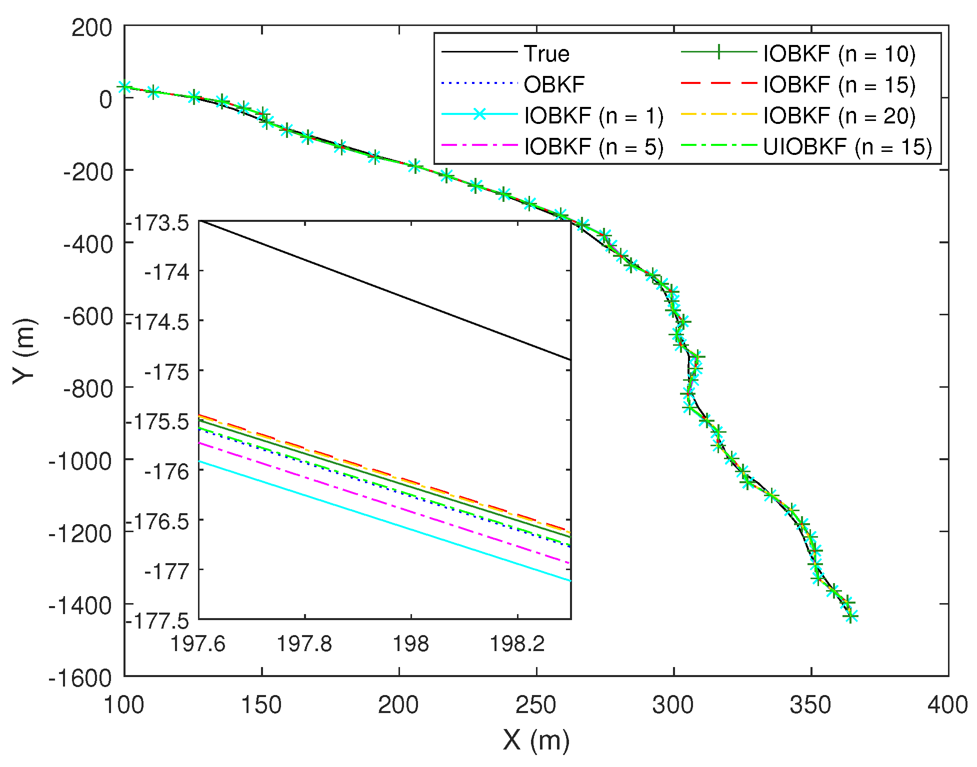
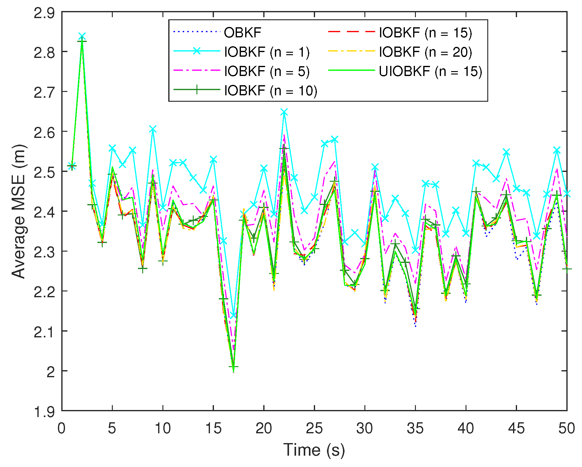
4. Numerical Simulations

In this section, target tracking examples are considered to verify the effectiveness of the proposed algorithm. For a linear state-space model

$$x_{k+1}=F_k{x}_k+w_k$$

(23)

$$y_k=H_k{x}_k+v_k$$

(24)

the state vector is $x_k={\left[p_x,{\dot{p}}_x,p_y,{\dot{p}}_y\right]}^T$, where $\left(p_x,p_y\right)$ and $\left({\dot{p}}_x,{\dot{p}}_y\right)$ represent the position and velocity in Cartesian coordinates, respectively. Model parameters are set as follows:

$$F_k=\left[\begin{array}{cccc}1& T& 0& 0\\ 0& 1& 0& 0\\ 0& 0& 1& T\\ 0& 0& 0& 1\end{array}\right],H_k=\left[\begin{array}{cccc}1& 0& 0& 0\\ 0& 0& 1& 0\end{array}\right]$$

where T is the sampling period. The covariance matrices of process and measurement noises are

$$Q_k^{{\theta }_1}=q\times \left[\begin{array}{cccc}{T}^3/3& T^2/2& 0& 0\\ T^2/2& T& 0& 0\\ 0& 0& T^3/3& T^2/2\\ 0& 0& T^2/2& T\end{array}\right],R_k^{{\theta }_2}=r\times \left[\begin{array}{cc}1& 0\\ 0& 1\end{array}\right]$$

where q and r are the unknown parameters. The initial state is $E\left[x_0\right]={\left[100,10,30,-10\right]}^T$ and $cov\left[x_0\right]=\mathrm{diag}\left(\left[25,2,25,2\right]\right)$, where $\mathrm{diag}\left(\nu \right)$ represents a diagonal matrix with diagonal elements $\nu$.

For comparison the OBKF, the proposed IOBKF, and the unweighted IOBKF (UIOBKF) are tested. The UIOBKF is the IOBKF without considering the weights of MCMC samples. In order to analyze the estimation performances of different algorithms, we use the average mean square-root error (MSE) as the performance metric, which is defined by

$${\mathrm{MSE}}_k\left(s\right)=\sqrt{\frac{1}{M}\sum _{i=1}^M\left({\left(s_{x,k}^i-{\widehat{s}}_{x,k}^i\right)}^2+{\left(s_{y,k}^i-{\widehat{s}}_{y,k}^i\right)}^2\right)}$$

(25)

where s denotes a position or a velocity variable, $s_k^i$ and ${\widehat{s}}_k^i$ denote the true and estimated values in the $i\mathrm{th}$ Monte Carlo trial, respectively, and M denotes the total number of Monte Carlo trials.

4.1. Time-Invariant Noise Statistics

In this case, the true noise parameters are set as $q=1.5$ and $r=0.5$, which are unknown in practice. The prior distributions of the noise statistical parameters q and r are set to be uniformly distributed in the ranges of $q\in \left[1,5\right]$ and $r\in \left[0.25,4\right]$, respectively.

The true and estimated trajectories in a single trial are shown in Figure 3, in which n is the size of the sliding window. The average position MSEs of different algorithms over $M=200$ Monte Carlo trials are shown in Figure 4 and their mean values are provided in

Table 1. Mean value of MSE and the average time for a single-step operation in different algorithms.

Algorithms	OBKF	IOBKF	IOBKF	IOBKF	IOBKF	IOBKF	UIOBKF
		(n = 1)	(n = 5)	(n = 10)	(n = 15)	(n = 20)	(n = 15)
MSE (m)	2.3369	2.4555	2.3852	2.3470	2.3373	2.3370	2.3423
Time (s)	0.0722	0.0248	0.0361	0.0439	0.0506	0.0562	0.0505

. It can be seen that the OBKF outperforms other algorithms, since the whole measurement sequence is used to estimate noise parameters. The estimation accuracy of the proposed IOBKF is related to the size of the sliding window. With the increase of the size of the sliding window, the estimation accuracy of the IOBKF gradually improves. When the size of sliding window is greater than 10, the estimation accuracy of the IOBKF for the state is close to that of the OBKF. In addition, when the size of the sliding window is fixed, i.e., $n=15$, our IOBKF is superior to the UIOBKF, in which the weights of MCMC samples are not considered.

The average time of single-step running of different algorithms is also shown in Table 1. It should be noted that the time consumption is closely related to the number of MCMC samples. In this paper, it is set to 600. The OBKF takes more time because it uses the whole measurement sequence to estimate noise parameters. Instead of the whole measurement sequence in the original OBKF, only n measurements are used in our algorithm, resulting in less computational cost.

The estimation results of noise parameters q and r are shown in Figure 5 and Figure 6, respectively. It can be seen that for all OBKFs, the estimation accuracy of the measurement noise parameter r is much better than that of the process noise parameter q. The main reason may be that parameter r is directly related to the observable measurements, while parameter q is a variable describing the disturbance of the hidden state. Although parameter q has a large deviation, it has little impact on the estimation accuracy of the state, since the Kalman filter can correct the one-step state prediction through the gain matrix and innovation.

In addition, from Figure 5 and Figure 6, we can see that our proposed IOBKF has a faster convergence speed than the OBKF and UIOBKF, since the weights of MCMC samples are taken into account in the former. When the size of the sliding window is greater than 15, the estimation accuracy of the IOBKF for noise parameters is close to that of the OBKF.

To summary, noise parameters are more sensitive to the size of the sliding window than the state. When considering the estimation accuracy of both the state and noise parameters, we choose 15 as the size of window. When only the estimation accuracy of the state is considered, we choose 10 as the size of window.

4.2. Time-Varying Noise Statistics

In this case, three scenarios are considered to verify the effectiveness of the proposed approach. The first is that both parameters q and r jump. The second is that only a single noise parameter r jumps. The last one is that the noise parameter r changes slowly.

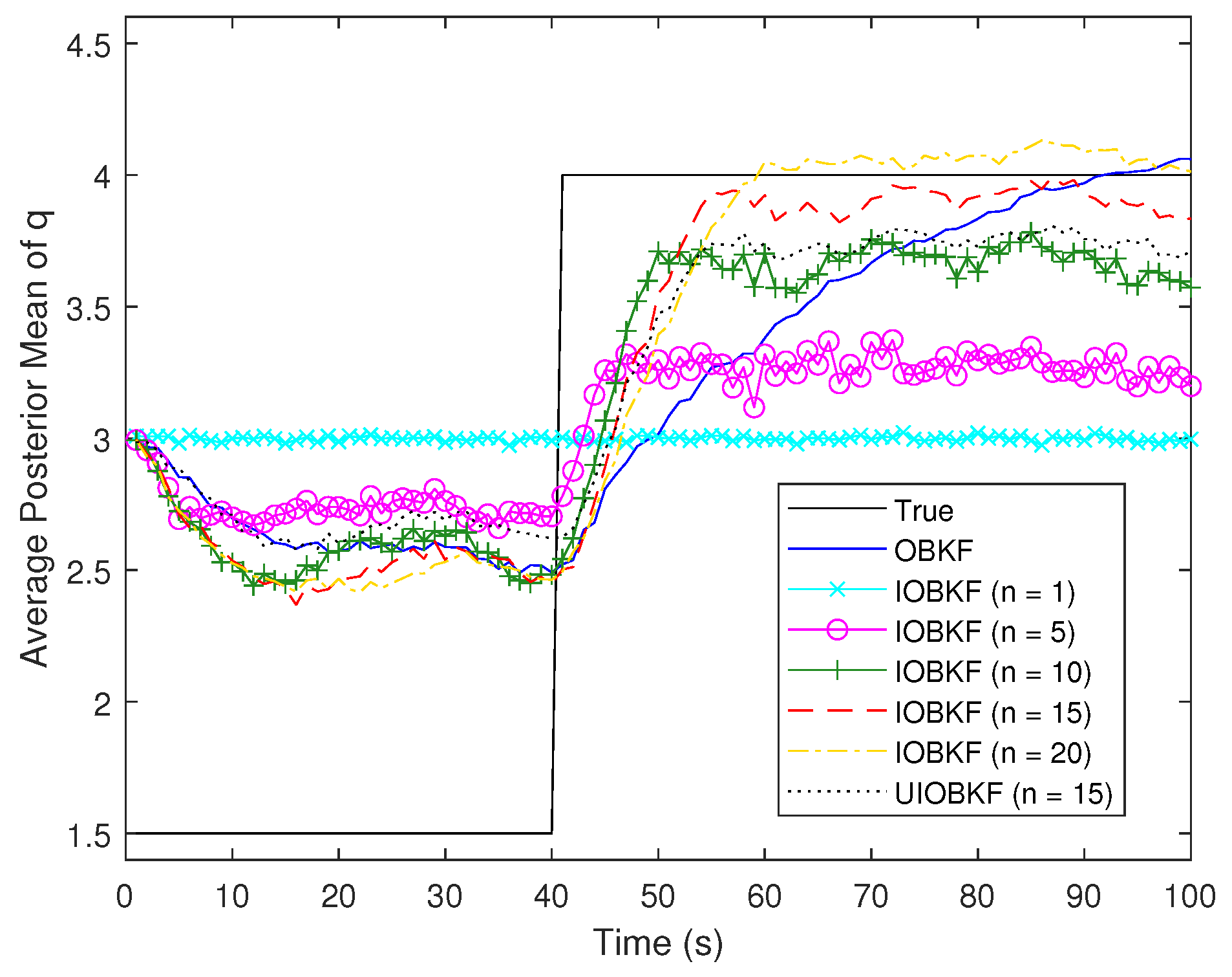
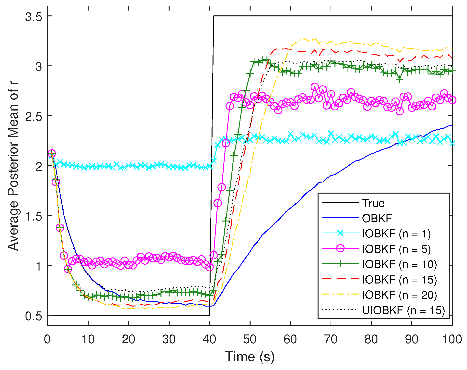
4.2.1. Both Noise Parameters q and r Jump

The true noise parameters are set as

$$q=\left\{\begin{array}{cc}1.5,& k\le 40\\ 4,& k>40\end{array},\right.r=\left\{\begin{array}{cc}0.5,& k\le 40\\ 3.5,& k>40\end{array}\right.$$

(26)

Their prior distributions are assumed to be uniformly distributed in the ranges of $q\in \left[1,5\right]$ and $r\in \left[0.25,4\right]$, respectively.

The true and estimated trajectories in a single trail are shown in Figure 7. The average position MSEs of different algorithms over $M=200$ Monte Carlo trials are shown in Figure 8 and their mean values over $40<n\le 100$ are provided in

Table 2. Mean value of MSE ($40<k\le 100$) and the average time for a single-step operation of different algorithms.

Algorithms	OBKF	IOBKF	IOBKF	IOBKF	IOBKF	IOBKF	UIOBKF
		(n = 1)	(n = 5)	(n = 10)	(n = 15)	(n = 20)	(n = 15)
MSE (m)	4.7037	4.7034	4.7302	4.7211	4.7180	4.7163	4.7206
Time (s)	0.1259	0.0235	0.0345	0.0429	0.0507	0.0580	0.0508

. It can be seen that the IOBKF performs better than the OBKF when noise parameters jump. The main reason is that the estimation accuracy of the OBKF for noise parameters q and r is very poor, as seen in Figure 9 and Figure 10, since it takes into account all previous measurements to update the posterior distribution of noise parameters. When the size of the sliding window is 1, the IOBKF has the fastest response, but its estimation results for parameters q and r are close to their mean values of the prior distributions. Considering the estimation accuracy of both the state and noise parameters, the size of the sliding window in the IOBKF can be chosen as 15. The average time of single-step running of different algorithms is also shown in Table 2, which is consistent with the result of the time-invariant noise, as shown in Table 1.

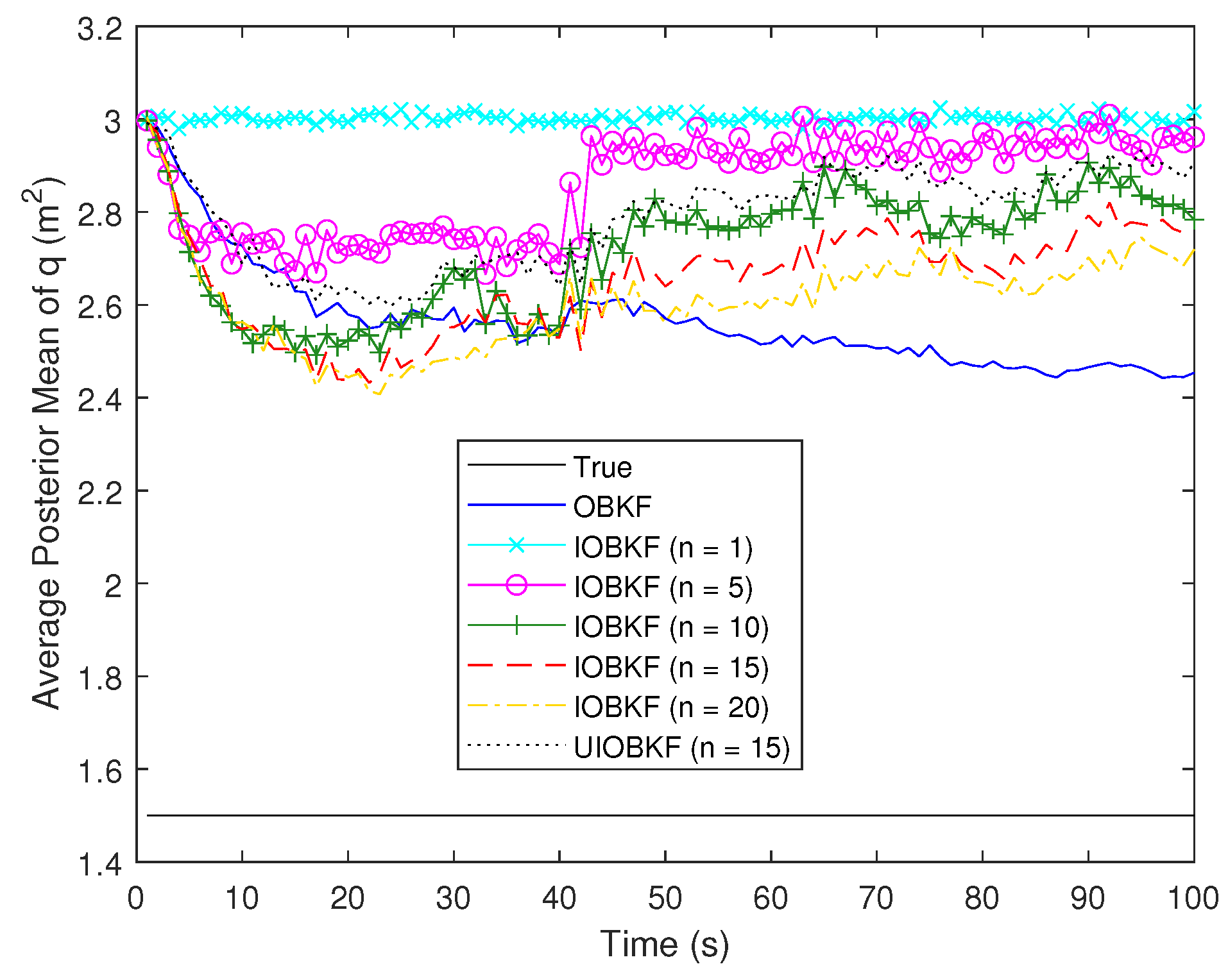
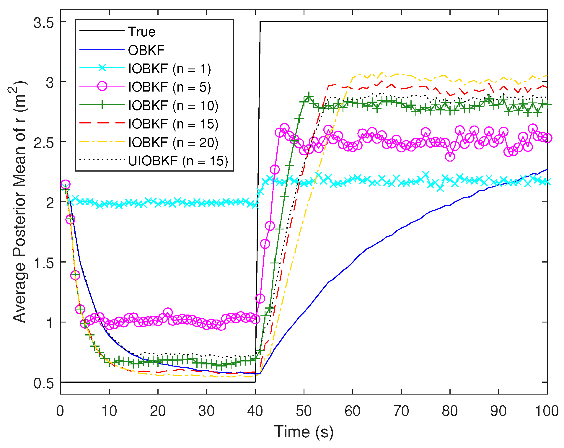
4.2.2. Noise Parameter q Is Time-Invariant and r Jumps

The true noise parameters are set as

$$q=1.5,r=\left\{\begin{array}{cc}0.5,& k\le 40\\ 3.5,& k>40\end{array}\right.$$

(27)

Their prior distributions are assumed to be uniformly distributed in the ranges of $q\in \left[1,5\right]$ and $r\in \left[0.25,4\right]$, respectively.

The results of the state estimation are not presented here because thay are similar to the results in Section 4.2.1. The estimation results of noise parameters q and r are shown in Figure 11 and Figure 12, respectively. It can be seen that for all OBKFs, the estimation accuracy of the measurement noise parameter r is still much better than that of the process noise parameter q. The main reason for this has been discussed in Section 4.1. Moreover, the process noise parameter q has less influence on the state estimation than the measurement noise parameter r. From Figure 12, the proposed IOBKF with $n\ge 15$ outperforms the OBKF. It should be emphasized that when the measurement noise parameter r jumps, the estimation of process noise parameter q also jumps, but the true value of q is a constant.

4.2.3. Noise Parameter q Is Time-Invariant and r Changes Slowly

The process noise parameter is a known constant, i.e., $q=1.5$, and the measurement noise parameter is set as

$$r=0.5+0.03\left(k-1\right)$$

(28)

where k is the time index. Its prior distribution is assumed to be uniformly distributed in the ranges of $r\in \left[0.25,4\right]$.

The estimation result of noise parameter r is shown in Figure 13. It can be seen that the proposed IOBKF with $n\ge 5$ performs better than the OBKF. However, when the noise parameter r changes slowly, a larger size of sliding window does not improve the estimation accuracy of the noise parameter. That is, the IOBKF with $n=20$ performs worse than the IOBKF with $n=15$.

5. Conclusions

In this paper, an improved OBKF is proposed to address the filtering problem for dynamic systems in the presence of inaccurate noise statistics. The sliding window technique is employed to computer the posterior distribution of noise parameters, which reduces the time consumption and improves the robustness to time-varying noise. The weights of samples generated by the MCMC approach are taken into account when calculating the posterior effective noise statistics, which simultaneously improves the estimation accuracy of noise parameters and the state. Several tracking scenarios are used to verify the effectiveness of the proposed algorithm. Especially in the case of time-varying noise statistics, the proposed algorithm performs better than the original OBKF in both running time and estimation accuracy.

The sliding window size plays an important role in the behavior of the IOBKF. It can be selected according to practical application by balancing the estimation accuracy and time consumption. In addition, it should be emphasized that for all OBKFs, the estimation accuracy of the measurement noise parameter r is much better than that of the process noise parameter q. The main reason may be that parameter r is directly related to the observable measurements, while parameter q is a variable describing the disturbance of the hidden state. Although parameter q has a large deviation, it has little impact on the estimation accuracy of the state, since the Kalman filter can correct the one-step state prediction through the gain matrix and innovation.

Finally, the limitation of the IOBKF is that each time, it still requires multiple measurements to estimate the posterior distribution of the noise parameters. Therefore, although the sliding window is used, the time consumption is still a non-negligible problem. Since these measurements originate from different times, the estimation accuracy of noise parameters at a certain time may be influenced. Future research work will be to study how to further improve the estimation accuracy of noise parameters, especially how to identify noise parameters at the current time by only using the measurement at the current time.

References

1. Bar-Shalom, Y.; Li, X.R.; Kirubarajan, T. Estimation with Applications to Tracking and Navigation: Theory, Algorthims and Software; Wiley: New York, NY, USA, 2001. [Google Scholar]
2. Chen, B.; Liu, X.; Zhao, H.; Principe, J.C. Maximum Correntropy Kalman Filter. Automatica 2017, 76, 70–77. [Google Scholar] [CrossRef] [Green Version]
3. Shan, C.; Zhou, W.; Jiang, Z.; Shan, H. A New Gaussian Approximate Filter with Colored Non-Stationary Heavy-Tailed Measurement Noise. Digit. Signal Process. 2021, 122, 103358. [Google Scholar] [CrossRef]
4. Zhang, G.H.; Han, C.Z.; Lian, F.; Zeng, L.H. Cardinality Balanced Multi-Target Multi-Bernoulli Filter for Pairwise Markov Model. Acta Autom. Sin. 2017, 43, 2100–2108. [Google Scholar]
5. Zandavi, S.M.; Chung, V. State Estimation of Nonlinear Dynamic System Using Novel Heuristic Filter Based on Genetic Algorithm. Soft Comput. 2019, 23, 5559–5570. [Google Scholar] [CrossRef]
6. Zhang, G.; Zeng, L.; Lian, F.; Liu, X.; Fu, N.; Dai, S. State Estimation for Dynamic Systems with Higher-Order Autoregressive Moving Average Non-Gaussian Noise. Front. Energy Res. 2022, 10, 990267. [Google Scholar] [CrossRef]
7. Kalman, R.E. A New Approach to Linear Filtering and Prediction Problems. J. Basic Eng. 1960, 82, 35–45. [Google Scholar] [CrossRef] [Green Version]
8. Anderson, B.D.; Moore, J.B. Optimal Filtering; Courier Corporation: New York, NY, USA, 2012. [Google Scholar]
9. Zhang, G.; Lian, F.; Han, C.; Chen, H.; Fu, N. Two Novel Sensor Control Schemes for Multi-Target Tracking via Delta Generalised Labelled Multi-Bernoulli Filtering. IET Signal Process. 2018, 12, 1131–1139. [Google Scholar] [CrossRef]
10. Zhang, G.; Lan, J.; Zhang, L.; He, F.; Li, S. Filtering in Pairwise Markov Model with Student’s t Non-Stationary Noise with Application to Target Tracking. IEEE Trans. Signal Process. 2021, 69, 1627–1641. [Google Scholar] [CrossRef]
11. Sarkka, S.; Nummenmaa, A. Recursive Noise Adaptive Kalman Filtering by Variational Bayesian Approximations. IEEE Trans. Autom. Contr. 2009, 54, 596–600. [Google Scholar] [CrossRef]
12. Kulikova, M.V. Square-Root Algorithms for Maximum Correntropy Estimation of Linear Discrete-Time Systems in Presence of Non-Gaussian Noise. Syst. Control Lett. 2017, 108, 8–15. [Google Scholar] [CrossRef] [Green Version]
13. Huang, Y.; Zhang, Y.; Wu, Z.; Li, N.; Chambers, J. A Novel Adaptive Kalman Filter with Inaccurate Process and Measurement Noise Covariance Matrices. IEEE Trans. Autom. Contr. 2018, 63, 594–601. [Google Scholar] [CrossRef]
14. Myers, K.; Tapley, B. Adaptive Sequential Estimation with Unknown Noise Statistics. IEEE Trans. Autom. Control 1976, 21, 520–523. [Google Scholar] [CrossRef]
15. Verdu, S.; Poor, H. Minimax Linear Observers and Regulators for Stochastic Systems with Uncertain Second-Order Statistics. IEEE Trans. Autom. Contr. 1984, 29, 499–511. [Google Scholar] [CrossRef]
16. Dehghannasiri, R.; Esfahani, M.S.; Dougherty, E.R. Intrinsically Bayesian Robust Kalman Filter: An Innovation Process Approach. IEEE Trans. Signal Process. 2017, 65, 2531–2546. [Google Scholar] [CrossRef]
17. Dehghannasiri, R.; Esfahani, M.S.; Qian, X.; Dougherty, E.R. Optimal Bayesian Kalman Filtering with Prior Update. IEEE Trans. Signal Process. 2018, 66, 1982–1996. [Google Scholar] [CrossRef]
18. Loeliger, H.A. An Introduction to Factor Graphs. IEEE Signal Process. Mag. 2004, 21, 28–41. [Google Scholar] [CrossRef] [Green Version]
19. Mao, Y.; Kschischang, F.R. On Factor Graphs and the Fourier Transform. IEEE Trans. Inform. Theory. 2005, 51, 1635–1649. [Google Scholar] [CrossRef]
20. Zhu, F.; Huang, Y.; Xue, C.; Mihaylova, L.; Chambers, J. A Sliding Window Variational Outlier-Robust Kalman Filter Based on Student’s t Noise Modelling. IEEE Trans. Aerosp. Electron. Syst. 2022. [Google Scholar] [CrossRef]
21. Lehmann, F.; Pieczynski, W. Reduced-Dimension Filtering in Triplet Markov Models. IEEE Trans. Autom. Control 2021, 67, 605–617. [Google Scholar] [CrossRef]
22. Ait-El-Fquih, B.; Desbouvries, F. Kalman Filtering in Triplet Markov Chains. IEEE Trans. Signal Process. 2006, 54, 2957–2963. [Google Scholar] [CrossRef]
Figure 1. Schematic diagram of calculation of the posterior distribution π θ | y 0 : k .
Electronics 11 03548 g001
Figure 2. The schematic representation of the proposed approach.
Electronics 11 03548 g002
Figure 3. True and estimated trajectories.
Electronics 11 03548 g003
Figure 4. Average MSEs of different algorithms.
Electronics 11 03548 g004
Figure 5. Estimation of noise parameter q.
Electronics 11 03548 g005
Figure 6. Estimation of noise parameter r.
Electronics 11 03548 g006
Figure 7. True and estimated trajectories.
Electronics 11 03548 g007
Figure 8. Average MSEs of different algorithms.
Electronics 11 03548 g008
Figure 9. Estimation of noise parameter q.
Electronics 11 03548 g009
Figure 10. Estimation of noise parameter r.
Electronics 11 03548 g010
Figure 11. Estimation of noise parameter q.
Electronics 11 03548 g011
Figure 12. Estimation of noise parameter r.
Electronics 11 03548 g012
Figure 13. Estimation of noise parameter r.
Electronics 11 03548 g013