
Brain Tumor Classification and Detection Using Hybrid Deep Tumor Network

 ,
, 

Abstract
:1. Introduction
- We propose a hybrid DL-TL model to identify two different kinds of brain malignancies (brain tumor) and (non-brain tumor (healthy).
- The proposed TL-DL detection technique shows superiority over current methods and has the highest accuracy on the Kaggle dataset. A huge number of tests are done with four distinct pre-trained DL models using TL strategies. Furthermore, in order to reveal the effectiveness of prediction performance of the proposed methods, compared with recent ML/DL and transfer learning model.
2. Related Works
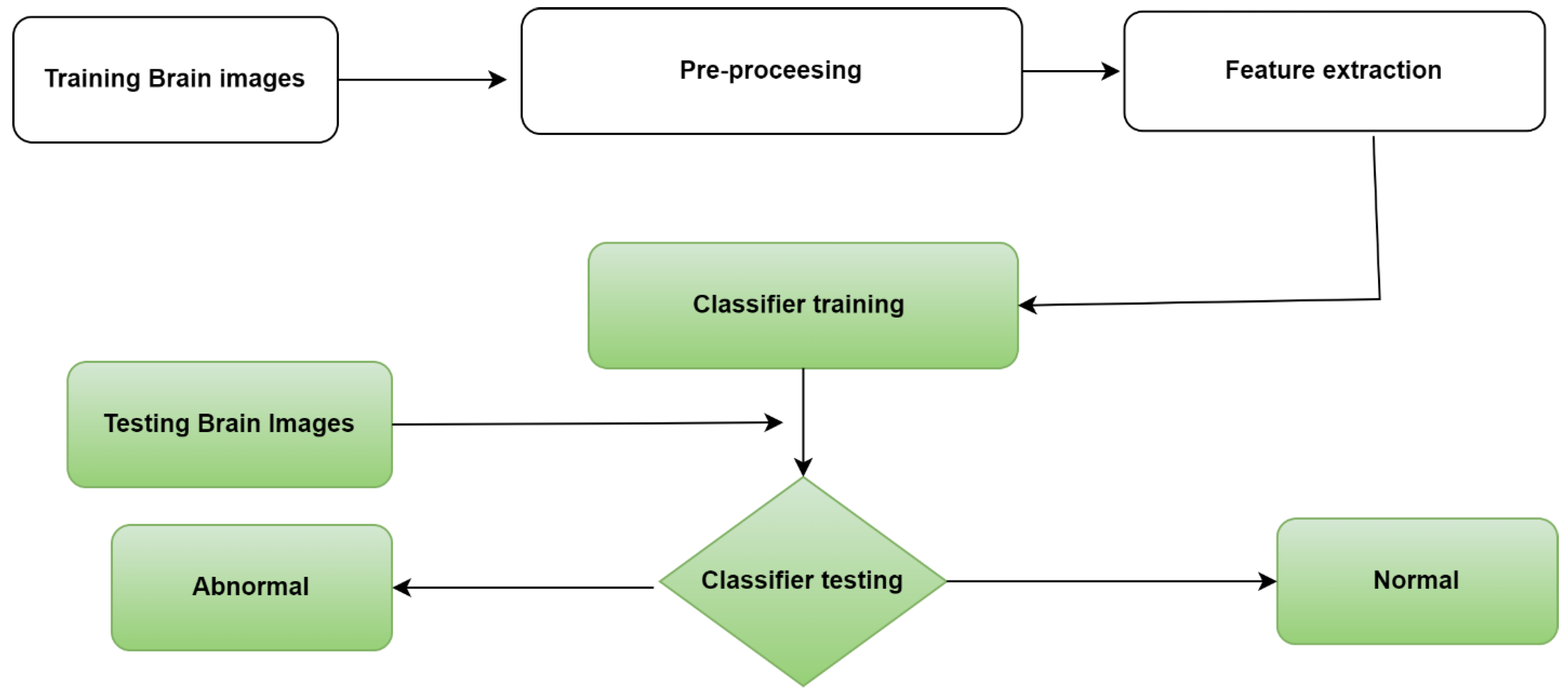
3. Methodology
3.1. Brain Tumor Kaggle Dataset
3.2. Preprocessing of the Dataset
3.3. Data Augmentation
- Position augmentationIn this process the position of the brain MRI images pixel is changed.
- ScalingIn scaling process, the brain images are resized.
- CroppingIn cropping process, a small portion of the brain MRI images is selected; here in this study we selected the center of the brain images.
- BrightnessIn this step the brightness of the brain images is changed from original to a lighter one.
3.4. Row Major Order
3.5. Proposed Model
3.6. Input Image Data
- Convolutional layerIn this layer, the two major inputs were image filter and matrix. The mathematical operation involved multiplying filter of the image generating input of the feature map.
- Activation layerIn this layer, the rectifier linear units (ReLUs) were used, which speeds up the training process and gives nonlinearity to the network model. The mathematical expression of the activation function is shown in Equation (1).ReLU_Act_Function (y) = y if y > 0
= 0 if y < 0.In the case of positive inputs (y), ReLU action function returns the value (y) as the output. However, when dealing with negative inputs, it returns a much smaller number that is equal to 0.01 times y. As a result, in this scenario, no neuron is rendered inactive, and we will no longer come across neurons that have died. - Batch normalization layersThe outputs that were created by the suggested convolution layers were used, and the batch normalization layer was applied to normalize them. The training duration of the recommended proposed model is shortened as a consequence of normalizing, which makes the process of learning both more efficient and more rapidly achieved. Normalization also makes the training period shorter.
- Pooling layerThe convolutional layer’s primary limitation is that it only captures the location-dependent features. Therefore, the categorization ends up being inaccurate if there is even a little shift in the position of the feature inside the image. By rendering the image more compact through the process of pooling, the network is able to bypass this constraint. As a result, the representation is now invariant to relatively few changes and particulars. Absolute pooling and average pooling were applied so that the characteristics might be linked to one another.
- Fully connected layerIn this layer, the features that were generated from the CLs are fed into the FC layers. In the FC layer, every node is connected with another node and makes the relation between an input image and its associate’s class. This layer implements SoftMax activation.
- Loss functionDuring training, this function (Y) must be reduced. After the image has been processed through all of the preceding layers, the output is calculated. The error rate is computed after comparing it to the expected outcome using the loss function. This technique is performed several times till its loss function is reduced. We used the binary cross-entropy as our loss function (BCE). The mathematical expression for BCE is shown in Equation (2).In binary classification, the actual value of y may only take on one of two potential forms: either 0 or 1. Therefore, in order to accurately determine the loss between the expected and actual results, it is necessary to compare the actual value, which can either be 0 or 1, with the probability that the input lines up with that category (where p(i) is the probability that the category is 1, and 1 − p(i) is the probability that the category is 0).
- SoftMax layerThe FC layer’s outcomes are more normally distributed because of the activation function. SoftMax performs the probabilistic computation for the network and generates work in positive values for each class.
- Classification LayerThe classification layer is indeed the model’s final layer to be demonstrated. This layer is utilized to generate the output by merging each input. As a consequence of the SoftMax AF, a posterior distribution was obtained [34].
- Grid search Hyperparameter optimizationGrid search hyperparameter is optimization approach that will methodically build and evaluate a model for each combination of algorithms parameters specified in a grid. In this problem, we tune the hypermeters by using grid search to find out the optimal hypermeters-based best classification performance. Furthermore, the grid search has optimal hyperparameter including epoch size = 100, Epsilon from 0.002, filter size = 1 × 1, batch size = 100 and the learning rate = 0.009. Furthermore, grid search optimization also used 10-fold cross validation. In 10-fold cross validation all the process, both the training and the test would be carried out only once within each set (fold). In order to avoid overfitting, 10-fold cross validation is the best technique to be used. k-fold validation reduces this variance by averaging over k different partitions, so the performance estimate is less sensitive to the partitioning of the data. In addition, in 10-fold cross validation process the one dataset is then split into 10 equal parts using a random number generator. Nine of those parts are put to use in training, while the remaining tenth is set aside for examination. We carry out this process a total of ten times, setting aside a different tenth of each iteration for evaluation each time.
3.7. Transfer Learning Model
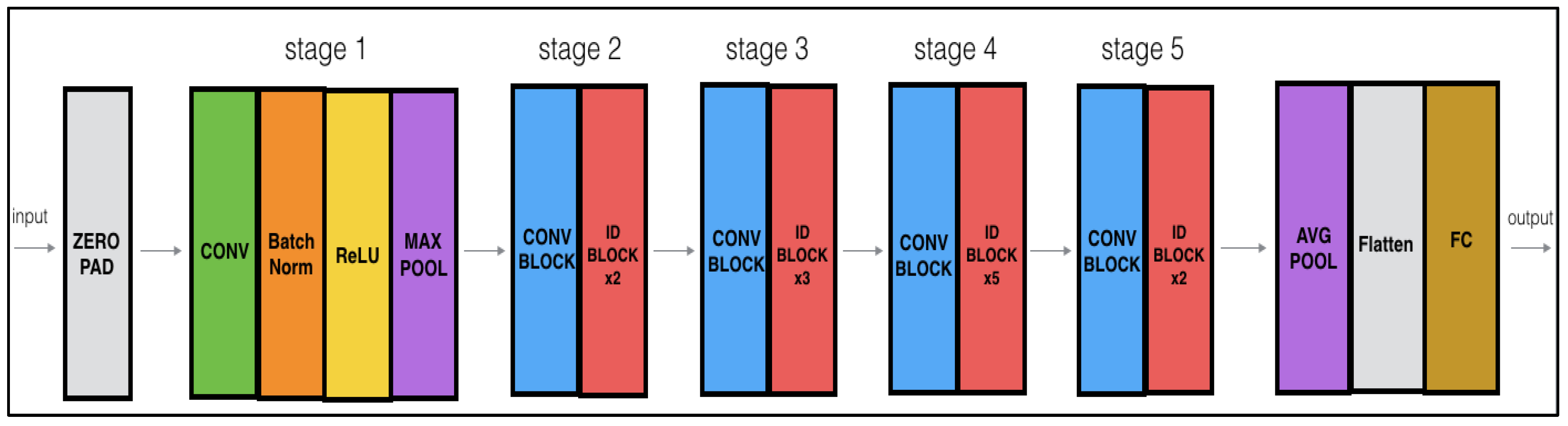
- ResNetThis model is related to Microsoft Research Center’s 50-layer Residual Network built in the research [60] ResNet employs shortcut connections to speed up training for improved service, which can decrease errors as complexity rises. Residual is linked to feature deduction. ResNet also addresses the issue of decreasing accuracy. Figure 5 depicts the ResNet model design.
- Mobile Net-V2As illustrated in the study [61], Mobile Net-V2 model has two types of blocks. The first block is made up of a series of linear bottleneck processes, whereas the second is a skip connection. Batch normalization, convolution, and a modified RLU are all included in both blocks. mobile-V2 has a total of 16 blocks.
- VGG-16Karen Simonyan and Andrew Zisserman of Oxford University’s Visual Geometry Group Lab proposed VGG 16 in the article “VERY DEEP CONVOLUTIONAL NETWORKS FOR LARGE-SCALE IMAGE RECOGNITION” in 2014. In the 2014 ILSVRC competition [61], this model took first and second place in the aforementioned categories as shown in Figure 6 [62].
- SqueezNetSqueeze Net is an 18-layer deep convolutional neural network. A pretrained variant of the network trained on over a thousand images of the ImageNet database may be loaded. As a consequence, the network has learnt detailed visual features for a diverse set of images. This method returns a Squeeze Net v1.1 network with similar accuracy as Squeeze Net v1.0 but fewer floating-point computations per prediction [63] as shown in Figure 7.
- Alex NetIn Alex Net, the network is divided into 11 different layers. The network has a significant number of layers, which makes feature extraction easier. In addition, the extensive number of factors has a negative influence on overall performance. The first layer that Alex Net has is called the convolution layer. The convolution layer is the third and last layer, coming after the maximum pooling and normalizing layers. The classification procedure comes to a close with the application of the SoftMax layer [64] as shown in Figure 8.
4. Result and Discussion
4.1. Experimental Setup
4.2. Evaluation Matrix
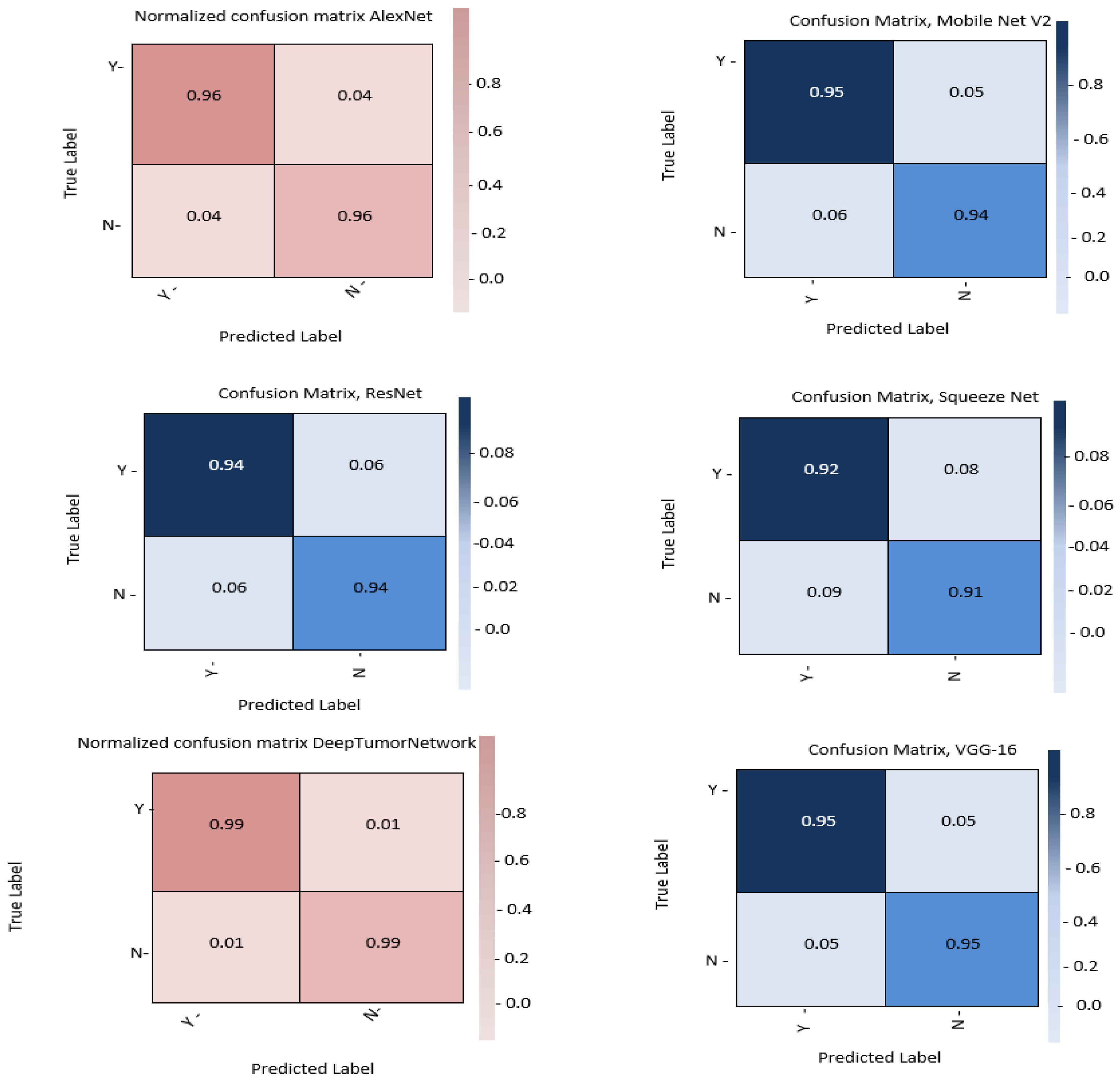
4.3. Confusion Matrix
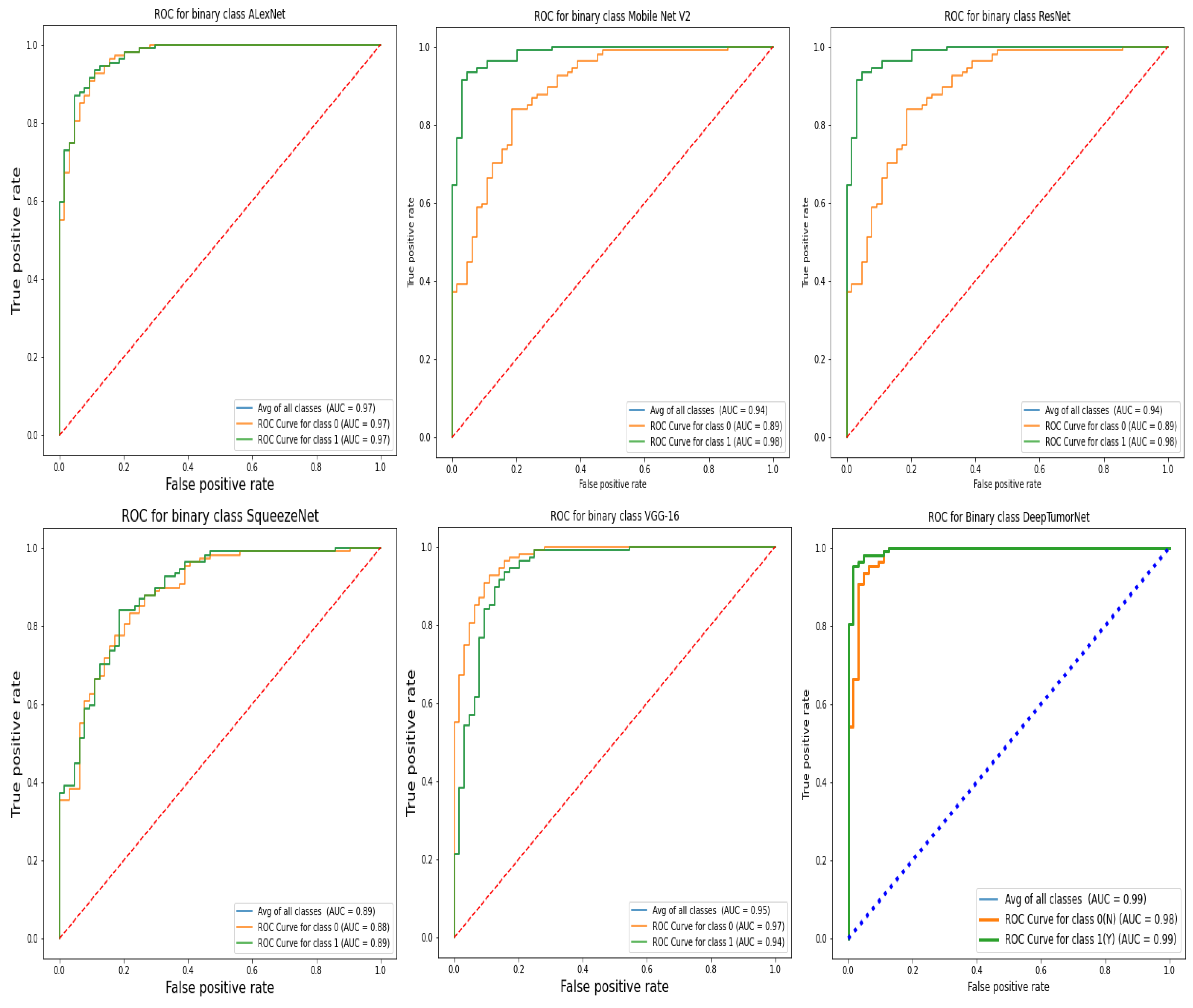
4.4. ROC Analysis
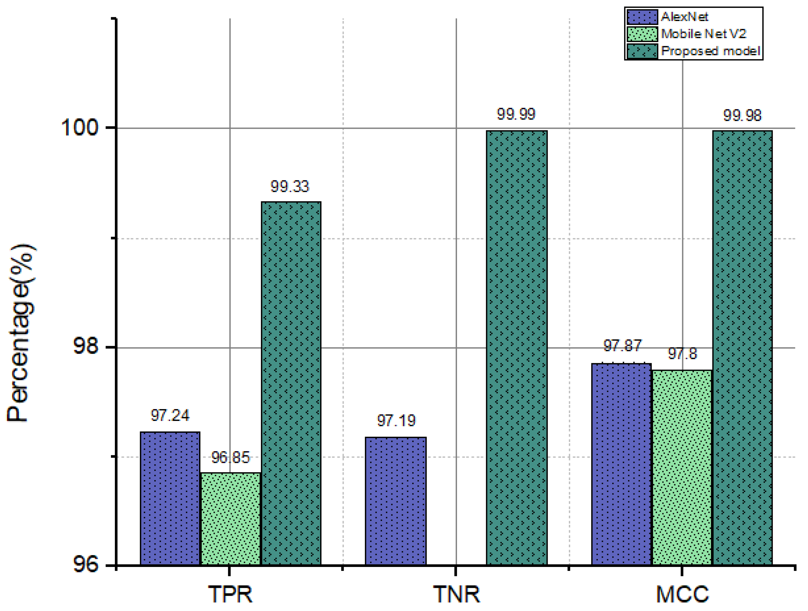
4.5. TNR, TPR, and MCC Analysis
4.6. Time Complexity (%)
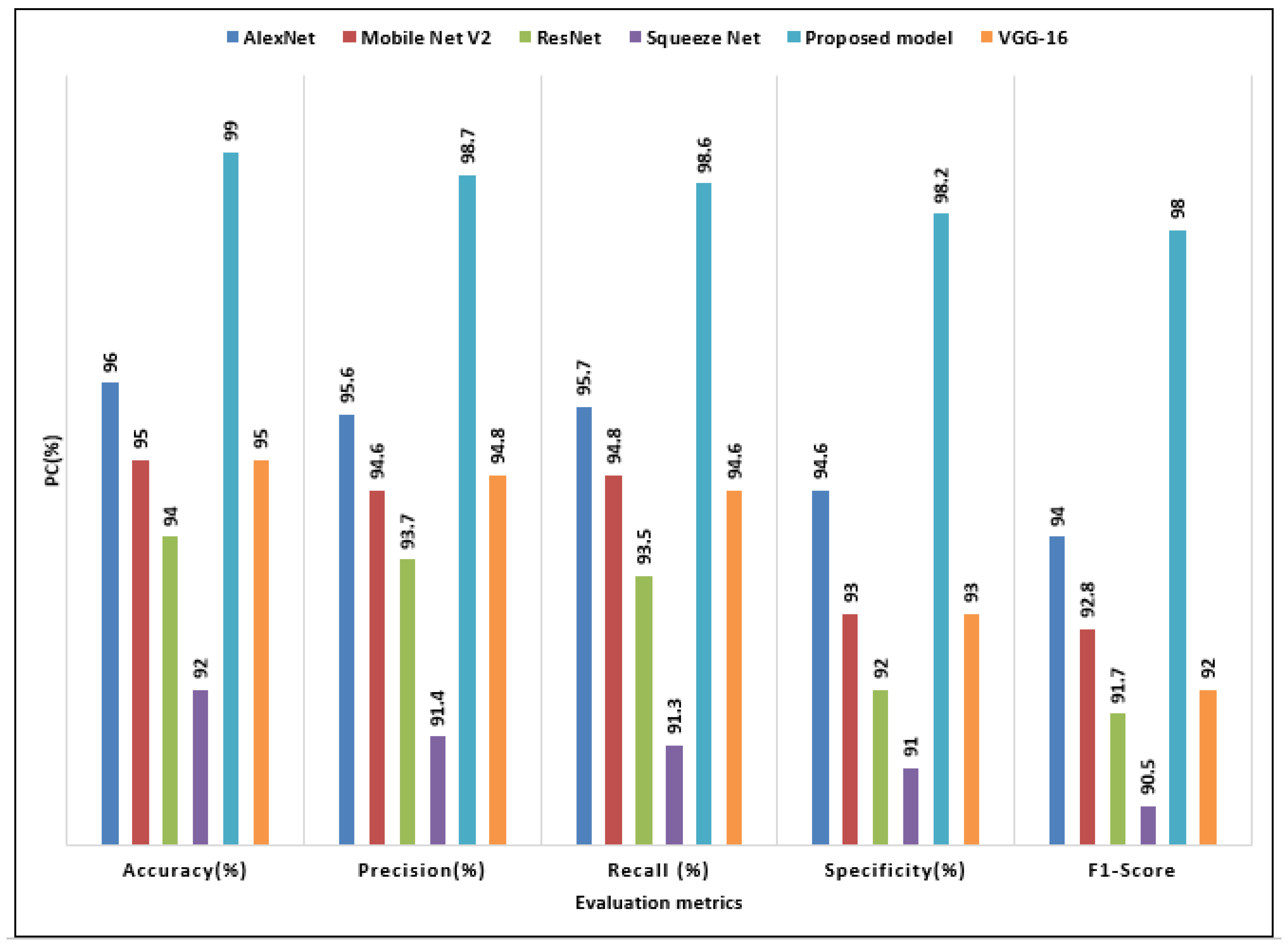
4.7. Comparative Results with Existing ML/DL Model
5. Conclusions
Author Contributions
Funding
Data Availability Statement
Acknowledgments
Conflicts of Interest
References
- Bush, N.A.O.; Susan, M.C.; Mitchel, S.B. Current and future strategies for treatment of glioma. Neurosurg. Rev. 2017, 40, 1–14. [Google Scholar] [CrossRef] [PubMed]
- Narkhede Sachin, G.; Khairnar, V.; Kadu, S. Brain tumor detection based on mathematical analysis and symmetry information. Int. J. Eng. Res. Appl. 2014, 4, 231–235. [Google Scholar]
- Praveen, G.B.; Agrawal, A. Hybrid approach for brain tumor detection and classification in magnetic resonance images. In 2015 Communication, Control and Intelligent Systems (CCIS); IEEE: Piscataway, NJ, USA, 2015. [Google Scholar]
- He, W.; Chen, F.; Dalm, B.; Kirby, P.A.; Greenlee, J.D. Metastatic involvement of the pituitary gland: A systematic review with pooled individual patient data analysis. Pituitary 2015, 18, 159–168. [Google Scholar] [CrossRef] [PubMed]
- DeAngelis, L.M. Brain tumors. N. Engl. J. Med. 2001, 344, 114–123. [Google Scholar] [CrossRef] [Green Version]
- Louis, D.N.; Perry, A.; Reifenberger, G.; Von Deimling, A.; Figarella-Branger, D.; Cavenee, W.K.; Ohgaki, H.; Wiestler, O.D.; Kleihues, P.; Ellison, D.W. The 2016 World Health Organization classification of tumors of the central nervous system: A summary. Acta Neuropathol. 2016, 132, 803–820. [Google Scholar] [CrossRef] [Green Version]
- Roy, S.; Nag, S.; Maitra, I.K.; Bandyopadhyay, S.K. A review on automated brain tumor detection and segmentation from MRI of brain. arXiv 2013, arXiv:1312.6150. [Google Scholar]
- Tutsoy, O.; Barkana, D.E.; Balikci, K. A novel exploration-exploitation-based adaptive law for intelligent model-free control approaches. IEEE Trans. Cybern. 2021, 1–9. [Google Scholar] [CrossRef] [PubMed]
- Rehman, A.; Naz, S.; Razzak, M.I.; Akram, F.; Imran, M. A deep learning-based framework for automatic brain tumors classification using transfer learning. Circuits Syst. Signal Process. 2020, 39, 757–775. [Google Scholar] [CrossRef]
- Wang, Y.; Zu, C.; Hu, G.; Luo, Y.; Ma, Z.; He, K.; Wu, X.; Zhou, J. Automatic tumor segmentation with deep convolutional neural networks for radiotherapy applications. Neural Process. Lett. 2018, 48, 1323–1334. [Google Scholar] [CrossRef]
- Visin, F.; Ciccone, M.; Romero, A.; Kastner, K.; Cho, K.; Bengio, Y.; Matteucci, M.; Courville, A. Reseg: A recurrent neural network-based model for semantic segmentation. In Proceedings of the IEEE Conference on Computer Vision and Pattern Recognition Workshops, Las Vegas, NV, USA, 26 June–1 July 2016. [Google Scholar]
- Mubashar, M.; Ali, H.; Grönlund, C.; Azmat, S. R2U++: A multiscale recurrent residual U-Net with dense skip connections for medical image segmentation. Neural Comput. Appl. 2022, 34, 17732–17739. [Google Scholar] [CrossRef]
- Raza, A.; Ayub, H.; Khan, J.A.; Ahmad, I.; SSalama, A.; Daradkeh, Y.I.; Javeed, D.; Ur Rehman, A.; Hamam, H. A Hybrid Deep Learning-Based Approach for Brain Tumor Classification. Electronics 2022, 11, 1146. [Google Scholar] [CrossRef]
- Ding, Y.; Zhang, C.; Lan, T.; Qin, Z.; Zhang, X.; Wang, W. Classification of Alzheimer’s disease based on the combination of morphometric feature and texture feature. In Proceedings of the 2015 IEEE International Conference on Bioinformatics and Biomedicine (BIBM), Washington, DC, USA, 9–12 November 2015; pp. 409–412. [Google Scholar]
- Ijaz, A.; Ullah, I.; Khan, W.U.; Ur Rehman, A.; Adrees, M.S.; Saleem, M.Q.; Cheikhrouhou, O.; Hamam, H.; Shafiq, M. Efficient algorithms for E-healthcare to solve multiobject fuse detection problem. J. Healthc. Eng. 2021, 2021, 9500304. [Google Scholar]
- Ahmad, I.; Liu, Y.; Javeed, D.; Ahmad, S. A decision-making technique for solving order allocation problem using a genetic algorithm. IOP Conf. Ser. Mater. Sci. Eng. 2020, 853, 012054. [Google Scholar] [CrossRef]
- Binaghi, E.; Omodei, M.; Pedoia, V.; Balbi, S.; Lattanzi, D.; Monti, E. Automatic segmentation of MR brain tumors images using support vector machine in combination with graph cut. In Proceedings of the 6th International Joint Conference on Computational Intelligence (IJCCI), Rome, Italy, 22–24 October 2014; pp. 152–157. [Google Scholar]
- Bahadure, N.B.; Ray, A.K.; Thethi, H.P. The comparative approach of MRI-based brain tumors segmentation and classification using genetic algorithm. J. Digit. Imaging 2018, 31, 477–489. [Google Scholar] [CrossRef]
- Zikic, D.; Glocker, B.; Konukoglu, E.; Criminisi, A.; Demiralp, C.; Shotton, J.; Thomas, O.M.; Das, T.; Jena, R.; Price, S.J. Forests for tissue-specific segmentation of high-grade gliomas in multi-channel MR. In Proceedings of the International Conference on Medical Image Computing and Computer-Assisted Intervention, Berlin/Heidelberg, Germany, 1 October 2012; pp. 369–376. [Google Scholar]
- Kaya, I.E.; Pehlivanlı, A.Ç.; Sekizkardeş, E.G.; Ibrikci, T. PCA based clustering for brain tumors segmentation of T1w MRI images. Comput. Methods Programs Biomed. 2017, 140, 19–28. [Google Scholar] [CrossRef]
- Nikam, R.D.; Lee, J.; Choi, W.; Banerjee, W.; Kwak, M.; Yadav, M.; Hwang, H. Ionic sieving through one-atom-thick 2D material enables analog nonvolatile memory for neuromorphic computing. Adv. Electron. Mater. 2021, 17, 2100142. [Google Scholar] [CrossRef]
- Zhang, J.P.; Li, Z.W.; Yang, J. A parallel SVM training algorithm on large-scale classification problems. In Proceedings of the 2005 International Conference on Machine Learning and Cybernetics, Guangzhou, China, 18–21 August 2005; pp. 1637–1641. [Google Scholar]
- Ye, F.; Yang, J. A deep neural network model for speaker identification. Appl. Sci. 2021, 11, 3603. [Google Scholar] [CrossRef]
- Ijaz, A.; Liu, Y.; Javeed, D.; Shamshad, N.; Sarwr, D.; Ahmad, S. A review of artificial intelligence techniques for selection & evaluation. IOP Conf. Ser. Mater. Sci. Eng. 2020, 853, 012055. [Google Scholar]
- Akbari, H.; Khalighinejad, B.; Herrero, J.L.; Mehta, A.D.; Mesgarani, N. Towards reconstructing intelligible speech from the human auditory cortex. Sci. Rep. 2019, 9, 874. [Google Scholar] [CrossRef] [PubMed] [Green Version]
- Szegedy, C.; Liu, W.; Jia, Y.; Sermanet, P.; Reed, S.; Anguelov, D.; Erhan, D.; Vanhoucke, V.; Rabinovich, A. Going deeper with convolutions. In Proceedings of the IEEE Conference on Computer Vision and Pattern Recognition, Boston, MA, USA, 7–12 June 2015; pp. 1–9. [Google Scholar]
- Harish, P.; Baskar, S. MRI based detection and classification of brain tumor using enhanced faster R-CNN and Alex Net model. Mater. Today Proc. 2020, 7, 770–778. [Google Scholar] [CrossRef]
- Saleem, S.; Amin, J.; Sharif, M.; Anjum, M.A.; Iqbal, M.; Wang, S.H. A deep network designed for segmentation and classification of leukemia using fusion of the transfer learning models. Complex Intell. Syst. 2021, 7, 3105–3120. [Google Scholar] [CrossRef]
- Howard, A.G.; Zhu, M.; Chen, B.; Kalenichenko, D.; Wang, W.; Weyand, T.; Andreetto, M.; Adam, H. Mobilenets: Efficient convolutional neural networks for mobile vision applications. arXiv 2017, arXiv:1704.04861. [Google Scholar]
- He, K.; Zhang, X.; Ren, S.; Sun, J. Deep residual learning for image recognition. In Proceedings of the IEEE Conference on Computer Vision and Pattern Recognition, Las Vegas, NV, USA, 27–30 June 2016; pp. 770–778. [Google Scholar]
- Zhang, X.; Zhou, X.; Lin, M.; Sun, J. Shufflenet: An extremely efficient convolutional neural network for mobile devices. In Proceedings of the IEEE Conference on Computer Vision and Pattern Recognition, Salt Lake City, UT, USA, 18–22 June 2018; pp. 6848–6856. [Google Scholar]
- Abiwinanda, N.; Hanif, M.; Hesaputra, S.T.; Handayani, A.; Mengko, T.R. Brain tumors classification using convolutional neural network. In World Congress on Medical Physics and Biomedical Engineering; Springer: Singapore, 2018; pp. 183–189. [Google Scholar]
- Ramzan, F.; Khan, M.U.G.; Rehmat, A.; Iqbal, S.; Saba, T.; Rehman, A.; Mehmood, Z. A deep learning approach for automated diagnosis and multi-class classification of Alzheimer’s disease stages using resting-state fMRI and residual neural networks. J. Med. Syst. 2020, 44, 37. [Google Scholar] [CrossRef]
- Anaraki, A.K.; Ayati, M.; Kazemi, F. Magnetic resonance imaging-based brain tumors grades classification and grading viaconvolutional neural networks and genetic algorithms. Biocybern. Biomed. Eng. 2019, 39, 63–74. [Google Scholar] [CrossRef]
- Noreen, N.; Palaniappan, S.; Qayyum, A.; Ahmad, I.; Imran, M.; Shoaib, M. A Deep Learning Model Based on Concatenation Approach for the Diagnosis of Brain Tumour. IEEE Access 2020, 8, 55135–55144. [Google Scholar] [CrossRef]
- Khan, H.A.; Jue, W.; Mushtaq, M.; Mushtaq, M.U. Brain tumour classification in MRI image using convolutional neural network. Math. Biosci. Eng. 2020, 17, 6203–6216. [Google Scholar] [CrossRef]
- Javeed, D.; Gao, T.; Khan, M.T.; Ahmad, I. A hybrid deep learning-driven SDN enabled mechanism for secure communication in Internet of Things (IoT). Sensors 2021, 21, 4884. [Google Scholar] [CrossRef]
- Ahmad, I.; Wang, X.; Zhu, M.; Wang, C.; Pi, Y.; Khan, J.A.; Khan, S.; Samuel, O.W.; Chen, S.; Li, G. EEG-based epileptic seizure detection via machine/deep learning approaches: A Systematic Review. Comput. Intell. Neurosci. 2022, 2022, 6486570. [Google Scholar] [CrossRef]
- Alanazi, A.K.; Alizadeh, S.M.; Nurgalieva, K.S.; Nesic, S.; Grimaldo Guerrero, J.W.; Abo-Dief, H.M.; Eftekhari-Zadeh, E.; Nazemi, E.; Narozhnyy, I.M. Application of Neural Network and Time-Domain Feature Extraction Techniques for Determining Volumetric Percentages and the Type of Two Phase Flow Regimes Independent of Scale Layer Thickness. Appl. Sci. 2022, 12, 1336. [Google Scholar] [CrossRef]
- Ahmad, S.; Ullah, T.; Ahmad, I.; Al-Sharabi, A.; Ullah, K.; Khan, R.A.; Rasheed, S.; Ullah, I.; Uddin, M.; Ali, M. A novel hybrid deep learning model for metastatic cancer detection. Comput. Intell. Neurosci. 2022, 2022, 8141530. [Google Scholar] [CrossRef]
- Ullah, N.; Khan, J.A.; Alharbi, L.A.; Raza, A.; Khan, W.; Ahmad, I. An Efficient Approach for Crops Pests Recognition and Classification Based on Novel DeepPestNet Deep Learning Model. IEEE Access 2022, 10, 73019–73032. [Google Scholar] [CrossRef]
- Wang, X.; Ahmad, I.; Javeed, D.; Zaidi, S.A.; Alotaibi, F.M.; Ghoneim, M.E.; Daradkeh, Y.I.; Asghar, J.; Eldin, E.T. Intelligent Hybrid Deep Learning Model for Breast Cancer Detection. Electronics 2022, 11, 2767. [Google Scholar] [CrossRef]
- Wang, Y.; Taylan, O.; Alkabaa, A.S.; Ahmad, I.; Tag-Eldin, E.; Nazemi, E.; Balubaid, M.; Alqabbaa, H.S. An Optimization on the Neuronal Networks Based on the ADEX Biological Model in Terms of LUT-State Behaviors: Digital Design and Realization on FPGA Platforms. Biology 2022, 11, 1125. [Google Scholar] [CrossRef] [PubMed]
- Khan, M.A.; Ahmad, I.; Nordin, A.N.; Ahmed, A.E.S.; Mewada, H.; Daradkeh, Y.I.; Rasheed, S.; Eldin, E.T.; Shafiq, M. Smart Android Based Home Automation System Using Internet of Things (IoT). Sustainability 2022, 14, 10717. [Google Scholar] [CrossRef]
- Ullah, N.; Khan, J.A.; Almakdi, S.; Khan, M.S.; Alshehri, M.; Alboaneen, D.; Raza, A. A Novel CovidDetNet Deep Learning Model for Effective COVID-19 Infection Detection Using Chest Radiograph Images. Appl. Sci. 2022, 12, 6269. [Google Scholar] [CrossRef]
- Zeineldin, R.A.; Karar, M.E.; Coburger, J.; Wirtz, C.R.; Burgert, O. DeepSeg: Deep neural network framework for automatic brain tumor segmentation using magnetic resonance FLAIR images. Int. J. Comput. Assist. Radiol. Surg. 2020, 15, 909–920. [Google Scholar] [CrossRef]
- Swati, Z.N.K.; Zhao, Q.; Kabir, M.; Ali, F.; Ali, Z.; Ahmed, S.; Lu, J. Brain tumor classification for MR images using transfer learning and fine-tuning. Comput. Med. Imaging Graph. 2019, 75, 34–46. [Google Scholar] [CrossRef]
- Maqsood, S.; Damasevicius, R.; Shah, F.M. An efficient approach for the detection of brain tumor using fuzzy logic and U-NET CNN classification. In International Conference on Computational Science and Its Applications; Springer: Cham, Switzerland, 2021. [Google Scholar]
- Gurbina, M.; Lascu, M.; Lascu, D. Tumor detection and classification of MRI brain image using different wavelet transforms and support vector machines. In Proceedings of the 2019 42nd International Conference on Telecommunications and Signal Processing (TSP), Budapest, Hungary, 1–3 July 2019; IEEE: Piscataway, NJ, USA, 2019; pp. 505–508. [Google Scholar]
- Rajinikanth, V.; Kadry, S.; Nam, Y. Convolutional-neural-network assisted segmentation and SVM classification of brain tumor in clinical MRI slices. Inf. Technol. Control 2021, 50, 342–356. [Google Scholar] [CrossRef]
- Amin, J.; Sharif, M.; Haldorai, A.; Yasmin, M.; Nayak, R.S. Brain tumour detection and classification using machine learning: A comprehensive survey. Complex Intell. Syst. 2021, 8, 3161–3183. [Google Scholar] [CrossRef]
- Badjie, B.; Ülker, E.D. A Deep Transfer Learning Based Architecture for Brain Tumor Classification Using MR Images. Inf. Technol. Control 2022, 51, 332–344. [Google Scholar] [CrossRef]
- Dvorák, P.; Menze, B. Local Structured prediction with convolutional neural networks for multimodal brain tumour segmentation. In MICCAI Multimodal Brain Tumour Segmentation Challenge (BraTS); Springer: Munich, Germany, 2015; pp. 13–24. Available online: http://people.csail.mit.edu/menze/papers/dvorak_15_cnnTumor.pdf (accessed on 10 October 2022).
- Irsheidat, S.; Duwairi, R. Brain Tumour Detection Using Artificial Convolutional Neural Networks. In Proceedings of the 2020 11th International Conference on Information and Communication Systems (ICICS), Irbid, Jordan, 7–9 April 2020; pp. 197–203. [Google Scholar] [CrossRef]
- Sravya, V.; Malathi, S. Survey on Brain Tumour Detection using Machine Learning and Deep Learning. In Proceedings of the 2021 International Conference on Computer Communication and Informatics (ICCCI), Coimbatore, India, 27–29 January 2021; pp. 1–3. [Google Scholar] [CrossRef]
- Kumar, S.; Mankame, D.P. Optimization drove deep convolution neural network for brain tumors classification. Biocybern. Biomed. Eng. 2020, 40, 1190–1204. [Google Scholar] [CrossRef]
- Maqsood, S.; Damaševičius, R.; Maskeliūnas, R. Multi-modal brain tumor detection using deep neural network and multiclass SVM. Medicina 2022, 58, 1090. [Google Scholar] [CrossRef] [PubMed]
- Waghmare, V.K.; Kolekar, M.H. Brain tumors classification using deep learning. In The Internet of Things for Healthcare Technologies; Springer: Singapore, 2021; Volume 73, pp. 155–175. [Google Scholar]
- Kaggle Official Web Page. Available online: https://www.kaggle.com/datasets//brain-tumor-detection// (accessed on 5 April 2022).
- Towardsdatascience Official Web Page. Available online: https://towardsdatascience.com/Resnet// (accessed on 5 April 2022).
- Towardsdatascience Official Web Page. Available online: https://towardsdatascience.com/mobilenet// (accessed on 5 April 2022).
- Geeksforgeeks Official Web Page. Available online: https://www.geeksforgeeks.org/vgg-16-cnn-model// (accessed on 5 April 2022).
- Towardsdatascience Official Web Page. Available online: https://towardsdatascience.com/review/ (accessed on 5 April 2022).
- Towardsdatascience Official Web Page. Available online: https://towardsdatascience.com/AlexNet// (accessed on 5 April 2022).


| Tumor Class | Images | Patients | Training Samples | Validation Samples | Testing Samples | Class Labels |
|---|---|---|---|---|---|---|
| BT Tumor | 1050 | 68 | 1050 | 250 | 250 | Yes (1) |
| No Tumor | 1050 | 70 | 1050 | 250 | 250 | No (0) |
| No. Layer | Epsilon | No of Filter | Filter Size |
|---|---|---|---|
| Conv2D_layer | 0.002 | 940 | 1 × 1 |
| Batch Norm layer | 0.001 | - | - |
| Clip ReLU layer | |||
| Group Conv2D layer | 940 | 3 × 3 | |
| Batch Norm layer | |||
| Clip ReLU layer | 0.002 | ||
| Conv2D_layer | 300 | 1 × 1 | |
| Batch Norm layer | 0.002 | ||
| Conv2D_layer | 1260 | 1 × 1 | |
| Glob AVG Pool layer | |||
| FC layer | |||
| SoftMax | |||
| Class Layer |
| Libraries | Keras, Pandas, Tensor, NumPy, |
|---|---|
| CPU | Intel, Cori7-processor |
| GPU | NAVID, 32 GB |
| Software | Python 3.7 |
| RAM | 16 GB |
| Publication | Classification Task | Models | Accuracy (%) | Precision (%) | Recall (%) | F1-Score (%) |
|---|---|---|---|---|---|---|
| This work | Binary classification task | Proposed model | 99.1 | 98.9 | 98.6 | 98 |
| [36] | CNN | 91.6 | 90.8 | 89.9 | 89.5 | |
| [33] | MobileNet-V2 | 94.9 | 93.6 | 92.8 | 92.6 | |
| [34] | KNN, SVM | 95.8 | 94.2 | 94 | 93.6 | |
| [27] | AlexNet | 93.6 | 92.6 | 92 | 91.4 | |
| [35] | VGG-16 | 92.9 | 91.5 | 921 | 90.9 | |
| [33] | M-SVM | 95.8 | 95 | 94.8 | 93 | |
| [34] | ANN | 93.7 | 92.5 | 91 | 90.50 |
Publisher’s Note: MDPI stays neutral with regard to jurisdictional claims in published maps and institutional affiliations. |
© 2022 by the authors. Licensee MDPI, Basel, Switzerland. This article is an open access article distributed under the terms and conditions of the Creative Commons Attribution (CC BY) license (https://creativecommons.org/licenses/by/4.0/).
Share and Cite
Amran, G.A.; Alsharam, M.S.; Blajam, A.O.A.; Hasan, A.A.; Alfaifi, M.Y.; Amran, M.H.; Gumaei, A.; Eldin, S.M. Brain Tumor Classification and Detection Using Hybrid Deep Tumor Network. Electronics 2022, 11, 3457. https://doi.org/10.3390/electronics11213457
Amran GA, Alsharam MS, Blajam AOA, Hasan AA, Alfaifi MY, Amran MH, Gumaei A, Eldin SM. Brain Tumor Classification and Detection Using Hybrid Deep Tumor Network. Electronics. 2022; 11(21):3457. https://doi.org/10.3390/electronics11213457
Chicago/Turabian StyleAmran, Gehad Abdullah, Mohammed Shakeeb Alsharam, Abdullah Omar A. Blajam, Ali A. Hasan, Mohammad Y. Alfaifi, Mohammed H. Amran, Abdu Gumaei, and Sayed M. Eldin. 2022. "Brain Tumor Classification and Detection Using Hybrid Deep Tumor Network" Electronics 11, no. 21: 3457. https://doi.org/10.3390/electronics11213457