Unlicensed Taxi Detection Model Based on Graph Embedding

Abstract

It is widely considered that unlicensed taxis pose a risk to public safety and interfere with the effective management of traffic. Significant human and material resources are expended by traffic control departments to locate these vehicles with limited success. This study suggests a smart, trajectory big data-based approach entitled Trajectory Graph Embedding-based Unlicensed Taxi Detection (TGE-UTD) to identify suspected unlicensed taxis and address this issue. The model implementation comprises three stages: first, the Automatic Number Plate Recognition (ANPR) data are transformed into a trajectory graph; second, a biased random walk is deployed to embed the trajectory graph; and finally, the set of vehicles similar to the known licensed taxis is obtained as the set of suspected unlicensed taxis using the cosine similarity of the vehicle embedding vector. Through precision evaluation and dimension reduction experiments, the performance of the walk model TGE-UTD is compared to that of the no-walk models Word2Vec and Doc2Vec in detecting large vehicles and taxis. TGE-UTD is observed to exhibit the best performance among the three models. This study pioneers the application of machine learning for feature extraction in detecting unlicensed taxis. The model proposed in the study can be deployed to detect unlicensed taxis; moreover, its application can be extended to detect other types of vehicles, providing traffic management departments with supporting vehicle detection information.

1. Introduction

Unlicensed taxis are private vehicles that transport passengers for a fee without formal operating authorization from the traffic police department. In recent years, unlicensed taxis have become more prevalent in urban areas. In a survey conducted by Tencent Technology on users’ experiences with unlicensed taxis, 80% of the nearly 25,000 respondents from more than 20 provinces reported that they frequently or occasionally ride in unlicensed taxis [1]. The operation of unlicensed taxis is associated with numerous concerns and concealed safety risks, such as inconsistent charging standards, deliberate detours, poor car conditions, insufficient liability safety insurance, and potential criminal risks, which endanger and harm passengers significantly. In China, the situation of unofficial taxis has been associated with a serious crime. In the early morning of 6 May 2018, an unlicensed taxi driver raped and murdered 21-year-old flight attendant Li Mingzhu [2].

It is common practice for traffic police to conduct spot checks for unlicensed taxis by setting up temporary checkpoints or conducting hot spot searches. However, these schemes are frequently time- and resource-intensive and have a low detection rate. Moreover, unlicensed taxis can evade such detection with relative ease. In addition, obtaining evidence of illegal conduct is difficult because unlicensed taxis are disguised as private vehicles.

Advanced technological devices such as road sensors, intersection cameras, and vehicle global positioning systems (GPS) have gathered substantial vehicle trajectory data pertaining to a variety of driving behavior traits. Recently, these trajectory data have been extensively used to address a variety of urban traffic issues with positive results. The mining of vehicle trajectory characteristics from these data and the detection of unlicensed taxis is a topic of active research. The trajectory data are subdivided into three additional categories: electronic registration identification (ERI) data [3], GPS data [4], and automatic number plate recognition (ANPR) data [5]. Only ANPR data do not require installation in moving vehicles, and they record the entire trajectory of moving vehicles. Due to the fact that ANPR data collection equipment is frequently installed at road intersections, the data provide only limited insight into the condition of urban road connectivity. The trajectory data from ANPR intersection cameras have been utilized extensively in traffic management to understand vehicle travel behavior and estimate travel time.

Existing models for detecting suspected unlicensed taxis are developed using similar steps. Step 1: analysis of the trajectory features of taxis and a feature extraction method is proposed; Step 2: a certain number of taxis and other vehicles are adopted as positive samples and negative samples from the original data set, the features of these samples are extracted utilizing the method proposed in Step 1, then a binary classification model is trained with the extracted features. Section 2.1 provides specific details.

Step 1 is a complex task due to the inefficiency of manually designing feature classification and extraction strategies. In practice, there are two types of trajectories for vehicles primarily involved in traffic: periodic and random. Taxis typically follow random trajectories, which have characteristics that are difficult to summarize and extract, and are therefore overlooked by researchers. Step 2 presents a challenge that the task of detecting unlicensed taxis cannot simply be viewed as a binary classification task. Prior studies utilized a high ratio of taxis to other vehicles when constructing the training set, whereas the ratio of taxis to other vehicles in the original data set may be quite low. This method of constructing the training set exposes the conundrum of uneven sampling of these two types of vehicles, which makes the binary classification task susceptible to producing incorrect results.

Therefore, this study designs and implements a graph embedding-based unlicensed taxi detection model, entitled Trajectory Graph Embedding-based Unlicensed Taxi Detection (TGE-UTD), based on an equal proportion sampling trajectory data set.

This study accomplishes the following:

• In the TGE-UTD, an ANPR dataset is transformed into a weighted trajectory graph, and vehicles are added as graph nodes. The graph fully depicts the driving trajectory and inclination of each vehicle.
• To collect the trajectory features of each vehicle equally in the TGE-UTD, a biased random walk trajectory sampling strategy on the map is proposed to augment the possible vehicle trajectories and obtain the trajectory features of each vehicle.
• A graph embedding machine learning model is trained according to the sampled trajectory to obtain the graph embedding vector of each vehicle in the TGE-UTD. The “similar-vehicle set” is obtained by setting the similarity threshold and comparing the similarity of vectors. Whereupon, potential unlicensed taxis are located and evaluated by comparing them to the set of similar vehicles.

In this study, a method is presented for transforming ANPR records into a trajectory graph, from which vehicle trajectory features are extracted utilizing machine learning, thereby reducing or even eliminating the need for manually designed feature extraction in previous studies. In addition, 100,000 vehicles are selected at random from the original data set to serve as the training set, after which taxis are identified as positive samples and other vehicles as negative samples. In contrast to the uneven sampling proportion in the training set that has been a problem in the existing literature, this method can make the proportion of vehicles in the training set consistent with that in the original data set, offering future researchers guidance for vehicle dataset sampling. In addition, the performance of three machine learning methods is compared, and it is demonstrated that TGE-UTD has the best performance in distinguishing between different types of vehicles, thereby providing enlightenment for methods regarding machine learning on a trajectory graph in vehicle detection tasks.

This study pioneers the application of machine learning for feature extraction in the detection of unlicensed taxis. Developed to identify unlicensed taxis, this method may also be applied to a wider range of vehicles.

2. Related Work

This section reviews the relevant literature on unlicensed taxi detection, trajectory graph construction, and graph embedding.

2.1. Unlicensed Taxi Detection

Previous studies designed vehicle feature extraction methods primarily through manual analysis of vehicle historical trajectories, extracted features from vehicle passing records, and selected a certain number of positive and negative samples for training binary classification models. The methods proposed by previous researchers for identifying unlicensed taxis are presented in

Table 1. Methods for identifying unlicensed taxis.

Model	Yuan et al. [6]	Wang et al. [7]	Tian et al. [8]	Chen et al. [9]
Year	2016	2017	2019	2021
Features	128	276	Two types	Four types
Positive Samples	6868	800	600	14,965
Negative Samples	3760	3200	400	104,798
Advantages	Split special time	Expand temporal and spatial features	Calculate path and time irregularity	Add features of points of interest
Disadvantages	No spatial features	Insufficient spatial features	Few feature types	No trajectory continuity

.

Yuan et al. [6] proposed a model for identifying unlicensed taxis that consists of a candidate selection model and a candidate refined model. This model counts the frequency of vehicle passing records and extracts the 128 vehicle classification features on this basis by leveraging 6868 licensed taxis as positive training samples and 3760 private vehicles as negative samples; however, it does not take into account the spatial and temporal characteristics of vehicles.

Wang et al. [7] enhanced the model developed by Yuan et al. [6] by increasing the number of vehicle classification features to 276 and comparing the effects of various classification models. This model uses 800 known unlicensed taxis and 3200 private vehicles as positive and negative samples, respectively. Nonetheless, the spatial characteristics extracted by the model are insufficient.

Tian et al. [8] proposed using abnormal trajectories and travel time to differentiate between licensed taxis and private vehicles. The training sets of various sizes containing training samples ranging from 100 to 1000 are selected, with 40% of the samples being negative and 60% positive. However, this method proposes only two types of vehicle classification features: path irregularity and time irregularity.

Chen et al. [9] extended the approach of Tian et al. [8] by incorporating feature analysis of points of interest of licensed taxis and random forest synthesis of multiple feature points for classification. In the training set, 14,965 taxis and 104,798 private cars serve as positive and negative samples, respectively. However, the model cannot differentiate between random and periodic trajectories because it does not account for the continuity of vehicle trajectories through intersections.

The preceding studies share a set of common shortcomings, which were introduced briefly in Section 1 and will be elaborated upon in this section.

Each of these studies conducted a manual analysis of the vehicle trajectory data sets, summarizing the techniques for extracting vehicle features. For instance, Yuan et al. [6] analyzed the passing records of vehicles and observed that taxis traveled in different manners than other vehicles during different time intervals; consequently, they proposed a method for extracting vehicle characteristics by counting the number of passing records during different time intervals. Tian et al. [8] analyzed the spatial and temporal features of vehicles, identifying the differences between commercial vehicles and non-commercial vehicles. Thereafter, they devised two formulas to calculate the path and time singularity of vehicles based on the feature differences. The aforementioned studies proceed by manually analyzing the trajectory data, then summarizing the vehicle features based on the knowledge of experts, and finally designing the method for extracting features and establishing the detection model. The inefficiency of the entire process makes it difficult to apply the methods proposed in these studies to the detection of other vehicles.

These studies utilize the training set consisting of a certain number of taxis, i.e., the positive samples, and non-taxi vehicles, i.e., the negative samples, selected from the original data set based on previous experience. Nonetheless, this type of sampling could expose the issue of uneven sampling of these two types of vehicles. As an illustration, consider the research by Chen et al. [9]. The ratio of taxi to non-taxi vehicles in the original data set is approximately 1 in 100, while in the training set, this ratio is approximately 1 in 7. The inconsistent ratio of positive samples to negative samples between the training set and the original data set would result in an unbalanced number of features collected from the two types of vehicles, making it easy for the binary classification model to differentiate between positive and negative samples. The taxi detection accuracy calculated by the model is falsely high. When the model is implemented in practical situations, a large number of private vehicles may be misidentified as taxis. Therefore, if a certain percentage of taxis are selected as positive samples, the same percentage of non-taxi vehicles should be selected as negative samples. If 14,965 taxis are selected as positive samples in the study by Chen et al. [9], then 1,496,500 instead of 104,798 private cars should be selected as negative samples.

In this study, machine learning is adopted, replacing manual data analysis for feature extraction, and the training set is constructed through random sampling to avoid the issue of an uneven sample proportion.

2.2. Trajectory Graph Construction

Huang et al. [10], Bogaerts et al. [11], and Hu et al. [12] utilize GPS data to construct trajectory maps and apply them to intelligent transportation’s downstream tasks. Their contribution consists of matching GPS data to maps. Typically, vehicle trajectory data are stored in relational databases. Anzum [13] developed a software system that enables data conversion and synchronization between a relational database and a graph database by defining nodes and relationships between nodes through manual dragging. Mueller et al. [14] proposed a simple method for converting dimension tables in relational databases into entities based on foreign key relations. The number of foreign keys was employed to transform the fact tables into entity relationships and intermediate entities in the graph database. Carlos et al. [15] proposed a unified meta-model (U-Schema) to summarize the logical patterns of diverse databases, such as relational, key-value, columnar, document, and graph, so that the data of diverse databases can be interconverted. Serin [16] proposed a mapping mode between a relational database and a graph database for public transportation networks, utilizing stations, routes, and vehicles as basic entities and station–route and vehicle–distance relationships as intermediate entities, and then connecting basic entities through intermediate entities to build a graph structure.

The present study develops a method for constructing graphs using ANPR data with vehicles and vehicle trajectories as the core, factoring in the characteristics of traffic big data and the requirements of downstream task characteristics.

2.3. Graph Embedding

Four categories comprise the majority of graph embedding models: matrix factorization, random walk, auto-encoder, and deep learning. Goyal and Ferrara [17] reviewed graph embedding and analyzed the time complexity of the methods of the preceding models. Graph embedding algorithms, whose time complexity is dependent on the edge set size, cannot be used in practical applications because the edge set size in the trajectory graph grows exponentially with time. DeepWalk [18] and Node2vec [19] with the random walk as the core and the DNGR [20] auto-encoder model are more suitable for these requirements. DNGR uses the random walk concept to generate the co-occurrence probability matrix from the graph input. Walk models refer to the aforementioned trajectory graph embedding models based on a random walk.

Huang et al. [21] proposed a trajectory embedding model that considered the intersections traversed by the vehicle to be words in the language and the vehicle trajectories to be sentences composed of words. The model employs the Word2Vec method for embedding learning, and the learning-derived intersection vectors are utilized for singular trajectory detection. Another trajectory embedding model was proposed by Kang et al. [22], which adopted the Doc2Vec method and added trajectory vectors to the model embedding learning. The trajectory embedding vectors obtained through learning are used to classify trajectories. The two models may also be employed for graph embedding, with the trajectories of a single vehicle constituting a subgraph of the entire trajectory graph. After graph embedding, the subgraph can express vehicle trajectory characteristics. No-walk models refer to trajectory graph embedding models without a random walk.

In contrast, the TGP-UTD model proposed in this study is a random walk-based graph embedding model. Section 4 compares it to the no-walk model employing vehicle detection and dimension reduction experiments.

3. Methodology

This section describes the datasets employed, the methods for detecting unlicensed taxis referred to as Trajectory Graph Embedding-based Unlicensed Taxi Detection (TGE-UTD), and the experimental design.

3.1. Dataset Description

This study utilizes the ANPR trajectory data from the intelligent transportation big data system in Changsha (a city in the Hunan Province of China), which encompasses the license plate information of passing vehicles and the time at which they passed through an intersection. These systems are deployed at intersections and can obtain information about all vehicles passing through intersections 24 h a day, in contrast to GPS devices, which are installed on individual vehicles. When a system detects a vehicle passing through the intersection, it takes a photograph of the vehicle, identifies the license plate and license plate color, and then transmits this data to the main server through the network. These systems generate approximately 30 million data points per day from over 700 intersections. The ANPR data set is not accessible to the public as it contains a large quantity of travel information involving personal privacy.

Table 2. A sample of the ANPR dataset.

License	Color	Intersection	Timestamp
XiangA****3	0	430100****38	2016/04/01 00:48:41
XiangA****3	0	430100****89	2016/04/01 00:55:31
XiangA****3	0	430100****86	2016/04/01 13:39:02
XiangA****3	0	430100****73	2016/04/01 13:41:42
XiangA****5	9	430100****15	2016/04/01 13:42:12

displays the ANPR records of a vehicle. In the table, “License ” and “Color” represent, respectively, the license plate and its color. In general, the color of the license plate is used to differentiate between small cars, large cars (including buses and construction vehicles), and special vehicles; 0 or 2 represent the blue license plate of small vehicles, whereas 9 represents the yellow license plate of large vehicles. The combination of the license and color of a vehicle can represent a unique vehicle. The number of the intersection where the ANPR equipment installed is denoted by “Intersection ”. A “Timestamp” denotes the passing time of a vehicle. Therefore, an ANPR record ($r_{ANPR}$) is represented in the following format:

$$r_{ANPR}=[License,Color,Intersection,Timestamp]$$

(1)

In April 2016 in Changsha, ANPR intersection cameras generated a dataset totaling 41 gigabytes and 170 million records. Errors in license plate recognition were discovered in the data set and attributed to intersection camera issues involving light, angle, and data transmission delays.

According to the transportation department’s license issuance policies, licensed taxi license plates with a color code of 0 or 2 are prefixed with XiangAT and XiangAX (Xiang is the abbreviation for Hunan Province). Since no rigorous restriction is in place on the use of XiangAT and XiangAX as license plate prefixes for private vehicles, the distinguishment of taxis from other vehicles proves challenging based solely on the license plate setting rule.

3.2. Unlicensed Taxi Detection Model

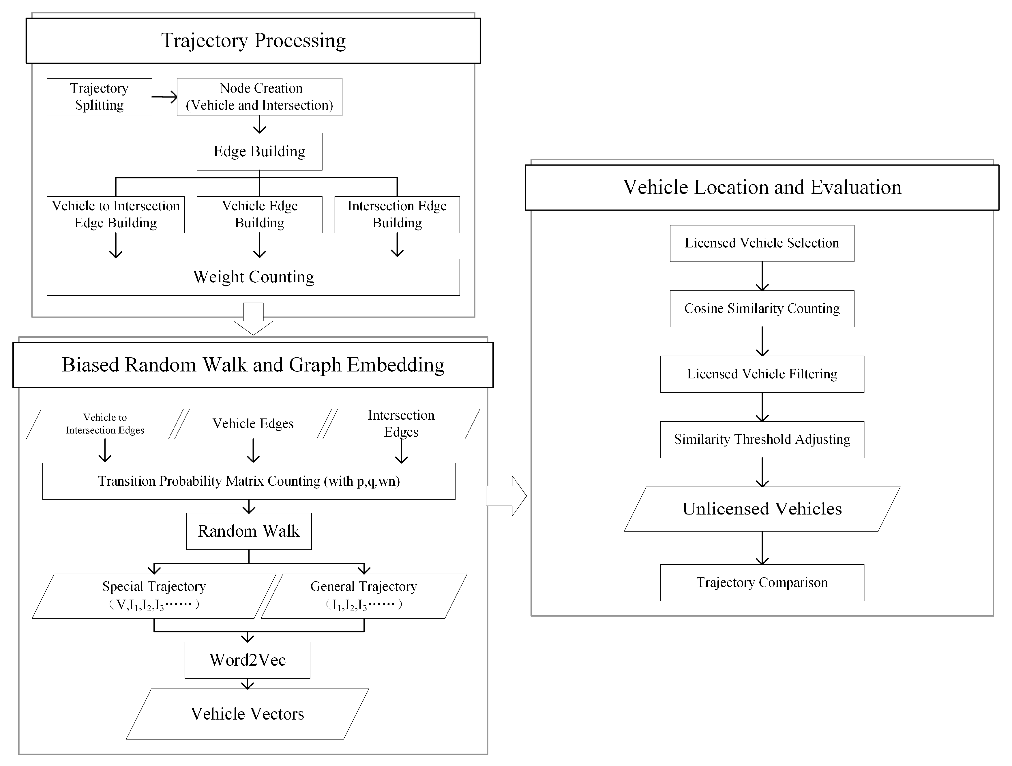
This section describes a method to identify and analyze unlicensed taxis based on the trajectory graph embedding model. Figure 1 outlines the process of Trajectory Graph Embedding-based Unlicensed Taxi Detection (TGE-UTD). This process comprises trajectory processing, biased random walk and graph embedding, and vehicle location and evaluation.

The trajectory processing part involves the construction of the trajectory graph. The vehicles and intersections are considered nodes of the graph. The vehicle trajectories are converted into graph edges, and the edge weight is calculated according to the vehicle passing frequency. The biased random walk and graph embedding part indicate the different transition matrix calculation methods used for various nodes in the trajectory graph. In the random walk, based on the idea of Node2Vec, the walk weight is adjusted to learn the vehicle trajectory features in a biased way, and then the word embedding method is used to train the graph embedding vector to obtain the vehicle embedding vector. In the vehicle location and evaluation part, the licensed taxi vector is taken as the baseline to find private cars with high cosine similarity [23] to the baseline vector. The real trajectories of the private cars found are manually compared with those of licensed taxis. If the two have a high similarity on the 3D trajectory diagram and a high percentage of common intersections, the found private cars are finally determined to be suspected unlicensed taxis.

3.2.1. Trajectory Processing

The trajectory of a vehicle ($Traj$) is determined by multiple records of the same vehicle according to the vehicle passing time and is represented as follows:

$$Traj=[I_1,I_2,I_3,\dots ,I_m]$$

(2)

$I_m$ represents the m-th intersection. If the time interval of a vehicle passing through two intersections exceeds 30 min [24], the vehicle has a parking behavior between the two intersections. Therefore, the trajectory is split into multiple sub-trajectories containing start and end points in the 30 min time interval. The resulting multiple sub-trajectories of vehicle V ($Traj{s}_V$) are described as follows:

$$Traj{s}_V=[Tra{j}_1,Tra{j}_2,Tra{j}_3,\dots ,Tra{j}_n]$$

(3)

$Tra{j}_n$ indicates the n-th trajectory. $Traj{s}_V$ is divided into edges forming the trajectory graph, and each edge contains the corresponding identifier of the passing vehicle. If the vehicle V travels from $I_i$ to $I_j$, an edge from node $I_i$ to node $I_j$ ($Edg{e}_{ij}^V$) is added to the trajectory graph, represented as follows:

$$Edg{e}_{ij}^V=(I_i,I_j,V,w_{V,ij})$$

(4)

If the vehicle travels from $I_i$ to $I_j$ multiple times, then the weight $w_{V,ij}$ is added to the $Edg{e}_{ij}^V$ based on the number of passing times. Therefore, the intersection edge set of the graph ($EdgeList$) is as follows:

$$EdgeList=[(I_1,I_2,w_{12}),(I_2,I_3,w_{23}),\dots ]$$

(5)

Each edge in the set represents the record of all cars passing through the two intersections, and w is the number of passes. The vehicle is also added to the graph as a node, and the edge set of vehicle V ($EdgeList\left(V\right)$) is represented as follows:

$$EdgeList\left(V\right)=[(V,I_i,w_{V,Vi}),(I_i,I_2,V,w_{V,i2}),(I_2,I_3,V,w_{V,23}),\dots ]$$

(6)

An example of the final trajectory graph is shown in Figure 2.

The graph describes two vehicles, Vehicle A and Vehicle B. Vehicle A has two trajectories, and Vehicle B has one. The vehicle node directly connects multiple intersection nodes, which are the starting points of each vehicle trajectory. For example, Vehicle A directly connects $I_1$ and $I_6$, the starting points of the Vehicle A trajectories. However, multiple directed edges with weights and vehicle identifiers exist between intersections. For example, there are edges with vehicle identifiers $\mathit{A\_Tra}{j}_1$ and $\mathit{B\_Tra}{j}_1$ between $I_2$ and $I_5$. The edge with vehicle identifier $\mathit{A\_Tra}{j}_1$ indicates that Vehicle A has a trajectory that goes through $I_2$ and $I_5$ sequentially, while the edge with vehicle identifier $\mathit{B\_Tra}{j}_1$ indicates that Vehicle B has a trajectory that goes through $I_2$ and $I_5$ sequentially. One trajectory of Vehicle A starts from $I_1$ and goes through $I_2$ and $I_5$ to the end point $I_7$. One trajectory of Vehicle B starts from $I_4$ and goes through $I_3$, $I_2$, and $I_5$ to the end point $I_7$. Both trajectories go through $I_2$, $I_5$, and $I_7$. Vehicle A also has a trajectory that starts at $I_6$ and ends at $I_7$, which is labeled $\mathit{A\_Tra}{j}_2$.

Based on the graph structure, the intersection transition probability of a vehicle can be calculated by the edges with specific identifiers between nodes, and that of all vehicles can be calculated by all edges between nodes, laying a foundation for the subsequent random walk.

3.2.2. Biased Random Walk and Graph Embedding

The traditional random walk model assumes a homogeneous graph. However, the trajectory graph constructed in this study contains vehicle nodes, intersection nodes, and edges between nodes marked with vehicle identifiers and is thus a heterogeneous graph. Therefore, a corresponding random walk strategy is proposed for this heterogeneous graph. As shown in the “Biased Random Walk and Graph Embedding” part in Figure 1, different calculation methods of the transition probability matrix are selected for various starting nodes.

The transition probability matrix is calculated by weighted sampling [25]. The intersection transition probability matrix shows the transition probability between intersection nodes, and the sampling weight is the number of times all vehicles pass between the nodes. The vehicle transition probability matrix indicates the transfer probability of a specified vehicle between intersection nodes, and the sampling weight is the number of times the vehicle passes between the nodes.

Parameters p and q are added in this study to control the breadth-first transition and depth-first transition tendencies based on the walk method of Node2Vec and conducts a random walk on the trajectory graph in a biased way. When $p<1$, the breadth-first transition probability increases, and then the starting node features increase. When $q<1$, the depth-first transition probability increases, and then the destination node features increase. Algorithm 1 describes the calculation process of the transition probability matrix. When the input graph G is the trajectory subgraph $G_V$ of the vehicle V, and $G_V$ contains only the trajectory of the vehicle V, the algorithm calculates the vehicle transition probability matrix of the vehicle V. When the input graph G contains the trajectories of all vehicles, the algorithm then calculates the intersection transition probability matrix.

Algorithm 1: Calculation of walk transition probability matrix.

The random walk is performed after calculating the walk transition probability matrix $W^{\prime }$. During this procedure, the scale of the specific experimental data determines the walk length ($wl$) and the number of walks ($wn$). As shown in Algorithm 2, the trajectory graph $G^{\prime }$ and the set of vehicle trajectory subgraphs $G_V^{\prime }$ are considered input. If the starting node is a vehicle, the vehicle transition probability matrix is used to impose a biased weighted random walk on $G_V$, and if the starting node is an intersection, the intersection transition probability matrix is used to impose a biased weighted random walk on graph G. Finally, the walk model produces the $wn$ random walk trajectories with a length of $wl$, which are used as learning samples for node embedding.

Most traditional feature learning models for vehicle trajectories directly use the original vehicle trajectories, but this study uses the random walk method to find potential vehicle trajectories. When used, this method increases the number of training samples and balances the number of trajectories between vehicles, enables TGE-UTD to capture the driving characteristics of vehicles with random trajectories, and makes TGE-UTD fault-tolerant for data sets with certain misrecognition records.

The random walk trajectories of each node are used as the training data, and the skip-gram model in Word2Vec is used to embed each node. TGE-UTD can obtain the node embedding vectors of all of the graph nodes, including the vehicle node vectors and intersection node vectors.

Algorithm 2: Random walk in graph.

3.2.3. Vehicle Location and Evaluation

A licensed taxi with a random trajectory is selected after all vehicle vectors have been obtained. The cosine similarity between the vectors of the licensed taxis and those of other vehicles is calculated by Equation (7). Vehicles having a high cosine similarity to the licensed taxis are found and added to the result set.

$$Similarity(A,B)=\frac{A·B}{\parallel A\parallel \parallel B\parallel }=\frac{{\sum }_{i=1}^n{A}_i\times B_i}{\sqrt{{\sum }_{i=1}^n{\left(A_i\right)}^2}\times \sqrt{{\sum }_{i=1}^n{\left(B_i\right)}^2}}$$

(7)

In the result set, the known licensed taxis are marked according to the plate setting rules, and the rest are suspected unlicensed taxis. The detection rate of suspected unlicensed taxis ($D{R}_{UT}$) is calculated by counting the number of known licensed taxis ($N_{LT}$) and the number of suspected unlicensed taxis ($N_{UT}$). The equation is as follows:

$$D{R}_{UT}=\frac{N_{UT}}{N_{UT}+N_{LT}}$$

(8)

A high $D{R}_{UT}$ value indicates that there are many suspected unlicensed taxis in the result set and the detection scope in the vector space is too large; therefore, some private cars with low similarity are misjudged as suspected unlicensed taxis. A low $D{R}_{UT}$ value may indicate that there are no suspected unlicensed taxis or that the detection scope is too small and only a small number of suspected illegal unlicensed taxis are detected, indicating that the detection scope should be expanded. This study sets a $D{R}_{UT}$ maximum threshold of 10%. It also develops an analysis method to control the detection rate of unlicensed taxis and improve the accuracy of the screening result of TGE-UTD. $RN$ (100 initially) is set to control the number of vehicles in the result set and ensure the efficiency of manual screening. Then, by adjusting $RN$, a similarity threshold $TH$ (0.8 initially) is set to control $D{R}_{UT}$. When $D{R}_{UT}$ is too high, $TH$ is increased to make the detection similarity higher and the detection scope smaller. When $D{R}_{UT}$ is too low and the similarity in the result set exceeds $TH$, $RN$ is increased to expand the detection scope, while $TH$ is unchanged.

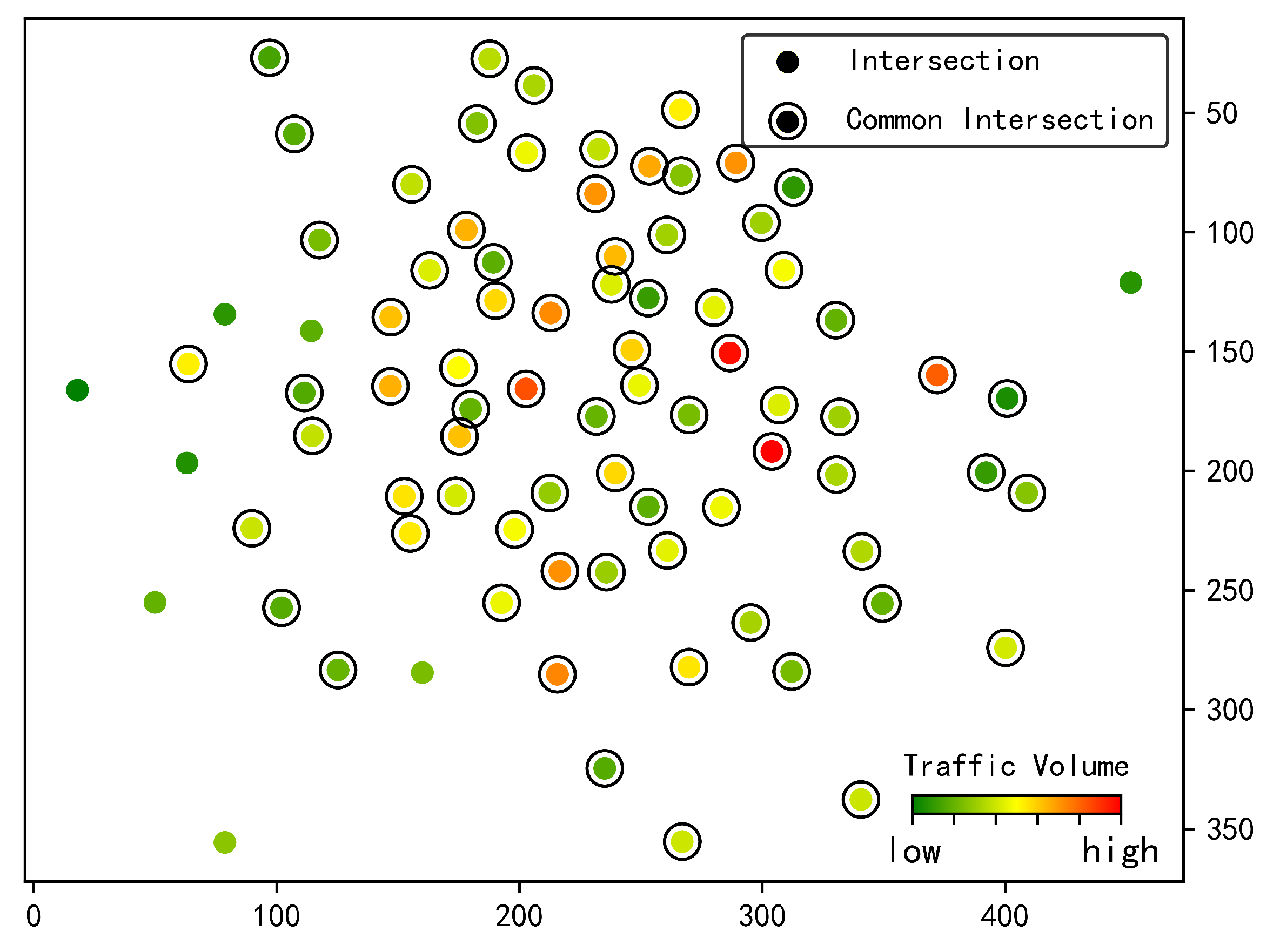
Suspected unlicensed taxis should also be screened manually. In this study, according to the original vehicle trajectories, a 3D trajectory diagram of the vehicles and a common intersection diagram with intersection traffic volume are constructed to assist in the determination of suspected unlicensed taxis. When comparing two vehicles, the 3D trajectory diagram can display the vehicles’ active regions and periods to allow manual verification of similar parts of their trajectories. The common intersection diagram shows the intersections passed by each vehicle, the intersections passed by both vehicles, and the traffic volume at the intersections. In this paper, in order to visually reflect the difference between the walk model and the no-walk model, t-SNE [26] is used to reduce the vector dimension, and different types of vehicles and detected unlicensed taxis are classified and colored.

3.3. Experimental Setting

3.3.1. Experimental Dataset Features

There are an estimated 3 million vehicles in Changsha, with approximately 6000 taxis representing 1/500 of the total. To ensure the viability and efficacy of the experiment, 100,000 vehicles were selected at random from the original data set to serve as the training data set for the experiment. The total number of trajectories in the data set is 4,144,612, and the frequency of passing vehicles is 9,498,874. This study did not obtain a specific taxi information record, and as such, taxis must be manually marked in accordance with the rules governing license issuance. In the training set, 4443 vehicles with a license plate prefix of XiangAT or XiangAX and a plate color code of 0 or 2 are marked as taxis, 16,729 vehicles with a plate color code of 9 are marked as large vehicles, and 78,828 unmarked vehicles are classified as other vehicles. As there is no rigorous restriction on private cars using the prefixes XiangAT and XiangAX on their license plates, it is possible that private cars with such license plate prefixes could be incorrectly identified as taxis. This study added a taxi marking rule requiring the number of vehicle passing records to be greater than 100 based on the experience of the traffic management department in detecting unlicensed taxis and the fact that the number of commercial vehicle passing records is typically greater than 100. The number of taxis in the training set was reduced from 4443 to 202 as a consequence of this rule. Finally, the training set contains 202 taxis, 16,729 large vehicles, and 83,069 other vehicles. Taxis account for 1/500 of the total. Thereby, the proportion of taxis in the training set matches the proportion in the original data set.

Figure 3 depicts the characteristics of trajectories and traffic volume in the training set. The value of trajectory length (represented by the number of intersections passed by the trajectory) is predominantly distributed below 10 in Figure 3a of the density distribution diagram for the training set. The density distribution diagram of the number of vehicle trajectories in the training set is depicted in Figure 3b, and the number of trajectories is distributed below 200. Figure 3c depicts the traffic volume during various training set time intervals. The volume distribution is consistent with the volume analysis results of Chen et al. [9], indicating that the vehicle trajectory features in this paper’s training set are consistent with previously analyzed trajectory features. Figure 3d portrays the traffic volume of each intersection in the training set (ranked from highest to lowest), indicating that approximately 50 intersections in the training set feature a high traffic volume.

3.3.2. Model Parameters

There are six main parameters in the proposed model TGE-UTD: p, q, $wn$, $wl$, $dim$, and $win$. In calculating the transition probability matrix, p and q control the breadth-first and depth-first transition probabilities of the random walk model. When $p<1$, the breadth-first transition probability increases and the walk focuses on the characteristics of the starting point of the trajectory; when $q<1$, the depth-first transition probability increases and the walk focuses on the characteristics of the end point of the trajectory. In the walking process, $wl$ and $wn$ control the walk length and the number of walks, respectively. As shown in Figure 3a, the trajectory length is distributed between 1 and 10, so $wl$ is set as 10. As shown in Figure 3b, the trajectory number density is mainly distributed between 1 and 125, so $wn$ is set at no less than 100. In the TGE-UTD training process, $dim$ and $win$ control the embedding vector dimension and the sliding window size of skip-gram, respectively. To comprehensively represent the relationship between vehicles and intersections, win is set as 10, and $dim$ is set as 128 by default. Therefore, the parameters to be adjusted in this experiment are p, q, and $wn$, as shown in

Table 3. Model parameters.

p	q	wn
0.1	2	100|200|400
0.5	2	100|200|400
1	1	100|200|400
2	0.1	100|200|400
2	0.5	100|200|400

.

A grid search method [27] is used to select the optimal values of p, q, and $wn$. When $p=0.1$ or $0.5$ and $q=2$, the breadth-first transition probability of the walk model increases; when $p=1$ and $q=1$, the transition probability of the walk model remains unchanged, and Node2Vec can be seen as DeepWalk; and when $p=2$, $q=0.1$ or $0.5$, the depth-first transition probability of the walk model increases. Besides, according to the number of trajectories distributed below 200 in Figure 3b, $wn$ is set to 100, 200, or 400.

3.3.3. Evaluation Metrics

To evaluate the performance of the vector embedding model, the average precision rate is used to describe the vector similarity performance of TGE-UTD for different vehicle types. First, the $TopN$ vehicles with the largest cosine similarity to the Vehicle V are found, and then the precision rate is calculated according to the number of $TopN$ vehicles of the same type as V. Finally, the average precision rate of all vehicles of this type ($Precisio{n}_{t,TopN}$) is calculated as follows:

$$\begin{array}{c}\hfill Type\left(V\right)=\left\{\begin{array}{cc}\hfill 0,& V is PrivateVehicle\hfill \\ \hfill 1,& V is LicensedTaxi\hfill \\ \hfill 2,& V is LargeVehicle\hfill \end{array}\right.\end{array}$$

(9)

$$\begin{array}{c}\hfill Precisio{n}_{t,TopN}=Mean(\frac{Count(Type\left(V_{t,i}\right)==Type\left(V_j\right))}{TopN})\\ \hfill V_j\in \left\{MostSimilar(V_{t,i},TopN)\right\}\end{array}$$

(10)

$Type\left(V\right)$ is a function to obtain the vehicle type of Vehicle V, t is a given vehicle type, $V_{t,i}$ is a vehicle of type t, and $MostSimilar(V_{t,i},TopN)$ is a function for finding the similar-vehicle set of $V_{t,i}$, which adds the $TopN$ vehicles with the largest similarity into this set. $TopN=10,20,50,100$ is used in this study.

4. Results and Analysis

In this section, through the precision evaluation and dimension reduction experiments, the TGE-UTD models proposed in the present study are evaluated and compared with different state-of-the-art baselines, Word2Vec and Doc2Vec models, based on entity embedding.

4.1. Training Results

The gensim module of Python 3.7 is used for vehicle vector training, and the average precision rate of the walk model TGE-UTD and no-walk models Word2Vec and Doc2Vec is calculated based on the evaluation matrix to characterize the learning ability of the models for vehicle trajectory features. Grid search is employed to determine the optimal TGE-UTD model parameters.

4.1.1. Large Vehicles

Similar to a typical vehicle with a periodic trajectory, the trajectories of large vehicles are predominantly circular, fixed, and characterized by relatively simple characteristics. Therefore, the average precision rate of large vehicles is high.

Figure 4 depicts the average precision rate for the walk model TGE-UTD and the no-walk models Word2Vec and Doc2Vec on the task of detecting large vehicles. The performance of TGE-UTD with various parameters is depicted at a magnified scale in the bottom right corner of each figure. At all $TopN$ value settings, both types of models perform well with the method for detecting large vehicles, as the average precision rate for all models is greater than 93%. The performance of TGE-UTD is only marginally inferior to that of the no-walk models.

Since no-walk models cannot fully extract the features of vehicles with random trajectories, this study employs the walk model to generate the possible trajectories of vehicles based on their historical trajectories, thereby enabling the full extraction of the features of vehicles with random trajectories. However, this method of generating trajectories will convert a number of vehicles with few trajectories into vehicles with periodic trajectories, thereby increasing the number of falsely positive samples of vehicles with periodic trajectories. As a result, for TGE-UTD, the average precision rate of large vehicles with periodic trajectories is decreased, while the ability to extract features from vehicles with random trajectories is enhanced.

It appears that the choice of p and q values has little effect on the average precision rate of large vehicles in TGE-UTD. In grid search, the average precision rate when $p=2$ and $q=0.1$ is only marginally superior to that under other $TopN$ value parameters. In addition, the performance of TGE-UTD is optimal under all parameters when $wn$ is set to 400.

4.1.2. Licensed Taxis

Taxi trajectories are predominantly low-periodic and random. These trajectories typically begin and end near commercial districts or transportation hubs. Due to taxi roaming, taxi routes are typically lengthy and uninterrupted.

Figure 5 illustrates the average precision rate for the walk model TGE-UTD and the no-walk models Word2Vec and Doc2Vec on the licensed taxi detection task. TGE-UTD outperforms Doc2Vec significantly. In overall terms, the performance of TGE-UTD is also superior to that of Word2Vec. Specifically, when $wn=200$ and $wn=400$, TGE-UTD performs better than Word2Vec, and their difference is more pronounced when $wn=400$ than when $wn=200$; however, when $wn=100$, TGE-UTD performs worse than Word2Vec. This is due to the fact that when $wn=200$ or 400, the TGE-UTD model executes a large number of random walks and generates rich taxi trajectories, including not only the historical trajectories of taxis, but also the new random trajectories generated by the model with reference to the history trajectories. These new random trajectories contain an abundance of potential vehicle characteristics, thereby assisting the model in extracting vehicle features. When $wn=100$, however, the TGE-UTD model generates only 100 walking trajectories for each vehicle, whereas the actual number of taxi trajectories in the training set is greater than 100. The insufficient number of features extracted by the model is due to the smaller number of taxi trajectories generated by walking than in the training set.

The choice of p and q values appears to have an effect on TGE-UTD. When $TopN=10$ or $TopN=20$, the model with parameters $p=0.5$ and $q=2$ achieves the best performance in a grid search, whereas when $TopN=50$ or 100, the model with parameters $p=2$ and $q=0.1$ achieves the best performance. In practice, there should be more than 20 taxis with similar random trajectories; consequently, the results of the average precision rate when $TopN=50$ or $TopN=100$ are more credible than when $TopN=10$ or $TopN=20$. Consequently, the optimal TGE-UTD parameters for the licensed taxi detection task are $p=2$ and $q=0.1$. Moreover, when $wn$ is 400, TGE-UTD has the best performance across all parameters. The average precision rate of taxis increases significantly as the number of random walks $wn$ increases.

4.2. Visualization Results

To enhance the set of suspected unlicensed taxis obtained by TGE-UTD, the 3D trajectory diagrams of both the known licensed taxis and the suspected unlicensed taxis were manually screened. Since the longitude and latitude data of intersections are not accessible to the public, the layout program heato in the graph drawing tool Graphviz [28] was employed to visualize a two-dimensional graph of vehicle trajectories. Then, a three-dimensional plot was constructed on the basis of this graph with the information of the time at which a vehicle passes through an intersection added in. As shown in Figure 6, the abscissas and ordinate denote the intersection location obtained by the visualization process and the applicate denotes the vehicle passing time. Trajectories on various dates are represented by lines of varying colors, while intersections are represented by dots. As shown in Figure 6, trajectories on various dates are represented by lines of varying colors, while intersections are represented by dots. Figure 6a depicts the 3D trajectory diagram of a licensed taxi (XiangAT**02), whereas Figure 6b depicts the 3D trajectory diagram of a suspected unlicensed taxi (XiangAJ**55). The trajectories of licensed taxi are more numerous than those of suspected unlicensed taxi, and the main trajectories of suspected unlicensed taxi are concentrated around the embedded abscissas 100 to 300 and the embedded ordinate 0 to 200, which overlap with the trajectories of licensed taxis to some extent.

Figure 7 depicts the intersection-passing records of a licensed taxi and a suspected unlicensed taxi. The intersection location denoted by the abscissas and ordinate in this figure is consistent with that in Figure 6. The dots represent the intersections passed by each vehicle, the dots with a circle represent the intersections passed by both vehicles, and the dot color represents the traffic volume of the intersections. Licensed taxis pass 81 intersections, while suspected unlicensed taxis pass 77 intersections. Both types of vehicles pass 75 intersections, of which 50 are among the top 50 intersections in terms of frequency of passage. Therefore, the suspected unlicensed taxi resembles the licensed taxi in that it primarily traverses intersections in the business district or high-volume traffic areas. We can therefore conclude that the suspected unlicensed taxi is a taxi that is illegal.

Figure 8 presents a visualization of vehicle vectors transformed by t-SNE. In Figure 8a, the vehicle vectors are calculated by Word2Vec, while in Figure 8b, the vehicle vectors are calculated by TGE-UTD. The closer two nodes are, the more similar they are. The abscissas and ordinate denote the location of the transformed vehicle vectors. The blue crosses represent large vehicles, the yellow dots represent intersections, the green dots represent private cars, the purple inverted triangles represent licensed taxis, and the red pentagons represent the suspected unlicensed taxis identified by Word2Vec or TGE-UTD.

The boundary between large vehicles and private cars can be explicitly seen in Figure 8a,b, reflecting that the two models perform well in distinguishing the periodic trajectory from other trajectories.

TGE-UTD significantly outperforms Word2Vec in extracting the trajectory characteristics of licensed taxis and detecting unlicensed taxis. In Figure 8a, taxis form an independent community, which is much further away from other communities, indicating that taxi trajectories learned by Word2Vec model have strong uniqueness and feature little randomness. This result is inconsistent with the actual situation of traffic, where taxis have random trajectories. Suspected unlicensed taxis, whose embedding vectors share a high cosine similarity with the vectors of licensed taxis, are dispersed in the private car community, which should be close to the taxi community and yet is actually far away, indicating that this model may misjudge these vehicles. The preceding results imply that the model has a limited capacity for learning vehicles with random trajectories. Comparatively, in Figure 8b, taxis congregate in the center of the largest private car community, indicating that private cars and taxis in this community have certain trajectory similarities, whereas vehicles with random trajectories have rich trajectory characteristics and are therefore likely to congregate in the center of the private car community. Therefore, this finding suggests that the vehicle vectors obtained by the TGE-UTD method can reflect the characteristic of random trajectories of taxis.

5. Conclusions

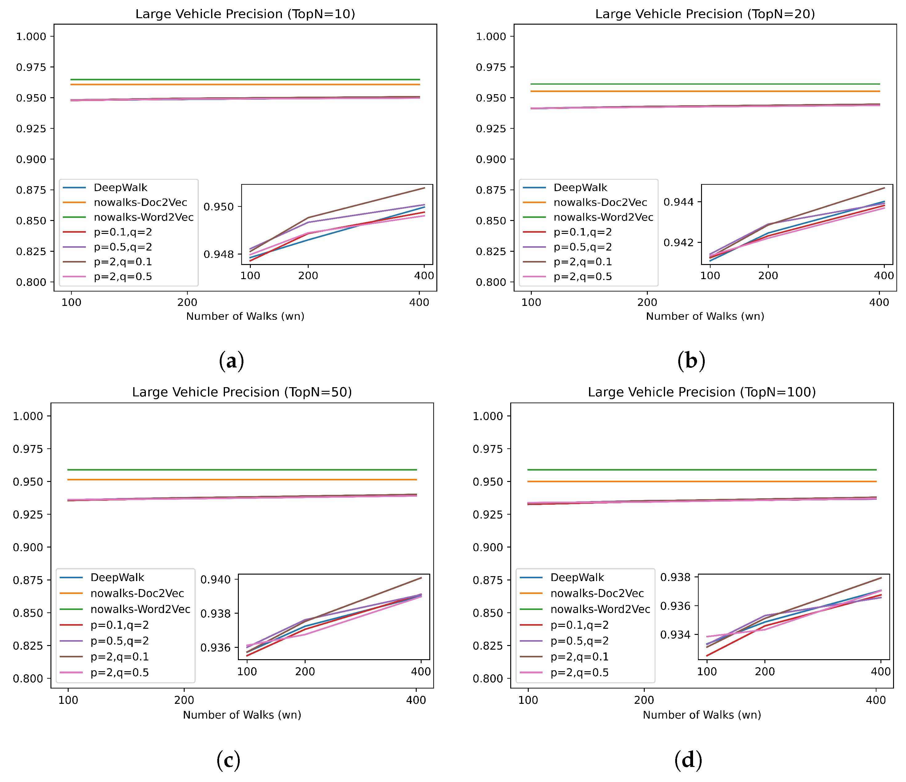
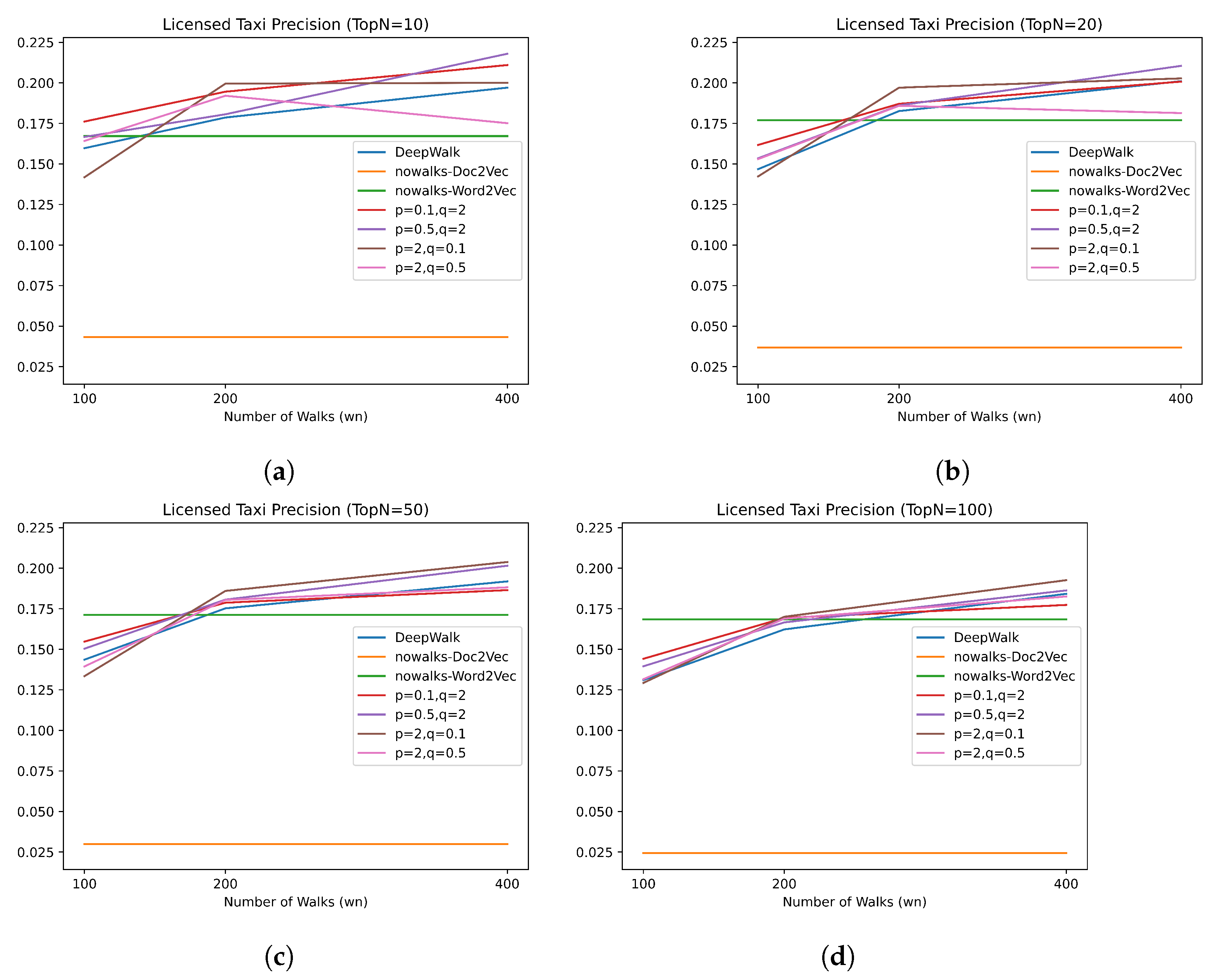
On the basis of real vehicle trajectory datasets, an unsupervised learning method for trajectory features is designed to detect suspected unlicensed taxis. The fundamental concept is to use a random walk to balance the number of vehicle trajectories and increase the number of possible trajectories. The average precision rate of the no-walk model and the walk model in detecting large vehicles and taxis is compared, and it is determined that the walk model can better learn trajectory features, and the vehicle vectors obtained by the model can more accurately represent the vehicle trajectory features. The performance of TGE-UTD under different parameters is addressed, and the optimal parameters are ascertained. The experimental results demonstrate that TGE-UTD can detect taxis and private cars with random trajectories and has a high precision rate for detecting large vehicles with periodic trajectories. Therefore, this study proposes a detection scheme for suspected unlicensed taxis by which 188 suspected unlicensed taxis are detected in the experimental data set. A 3D trajectory diagram and a common intersection diagram are deployed to evaluate the detection results.

Traditional methods for detecting suspect unlicensed taxis rely heavily on the manual analysis and extraction of suspicious trajectory features by experts. However, the proposed TGE-UTD can automatically learn trajectory features and successfully accomplish the detection task. It has the ability to identify suspected unlicensed taxis and other types of vehicles, and thereby offers a decision-making and information foundation for traffic management departments.

References

1. 80% of the Respondents Had Ridden in “Black Cars” and Called for Market Liberalization. Available online: https://cloud.tencent.com/developer/article/1042178 (accessed on 17 October 2022).
2. The Murder of the Flight Attendant Li Mingzhu. Available online: http://www.hxnews.com/news/itkj/kjqy/201805/12/1518019_2.shtml (accessed on 17 October 2022).
3. Zheng, L.; Xia, D.; Chen, L.; Sun, D. Understanding citywide resident mobility using big data of electronic registration identification of vehicles. IEEE Trans. Intell. Transp. Syst. 2019, 21, 4363–4377. [Google Scholar] [CrossRef]
4. Tang, J.; Liu, F.; Wang, Y.; Wang, H. Uncovering urban human mobility from large scale taxi GPS data. Phys. Stat. Mech. Appl. 2015, 438, 140–153. [Google Scholar] [CrossRef]
5. Patel, C.; Shah, D.; Patel, A. Automatic number plate recognition system (anpr): A survey. Int. J. Comput. Appl. 2013, 69, 21–33. [Google Scholar] [CrossRef]
6. Yuan, W.; Deng, P.; Taleb, T.; Wan, J.; Bi, C. An unlicensed taxi identification model based on big data analysis. IEEE Trans. Intell. Transp. Syst. 2015, 17, 1703–1713. [Google Scholar] [CrossRef]
7. Wang, Y.; Fan, X.; Liu, X.; Zheng, C.; Chen, L.; Wang, C.; Li, J. Unlicensed taxis detection service based on large-scale vehicles mobility data. In Proceedings of the 2017 IEEE International Conference on Web Services (ICWS), Honolulu, HI, USA, 25–30 June 2017; pp. 857–861. [Google Scholar]
8. Tian, Y.; Yang, J.; Lu, P. Unlicensed taxi detection algorithm based on traffic surveillance data. In Proceedings of the 5th ACM SIGSPATIAL International Workshop on the Use of GIS in Emergency Management, Chicago, IL, USA, 5 November 2019; pp. 1–7. [Google Scholar]
9. Chen, L.; Zheng, L.; Xia, L.; Liu, W.; Sun, D. Detecting and analyzing unlicensed taxis: A case study of Chongqing City. Phys. Stat. Mech. Appl. 2021, 584, 126324. [Google Scholar] [CrossRef]
10. Huang, X.; Zhao, Y.; Ma, C.; Yang, J.; Ye, X.; Zhang, C. TrajGraph: A graph-based visual analytics approach to studying urban network centralities using taxi trajectory data. IEEE Trans. Vis. Comput. Graph. 2015, 22, 160–169. [Google Scholar] [CrossRef] [PubMed]
11. Bogaerts, T.; Masegosa, A.D.; Angarita-Zapata, J.S.; Onieva, E.; Hellinckx, P. A graph CNN-LSTM neural network for short and long-term traffic forecasting based on trajectory data. Transp. Res. Part C Emerg. Technol. 2020, 112, 62–77. [Google Scholar] [CrossRef]
12. Hu, S.; Gao, S.; Wu, L.; Xu, Y.; Zhang, Z.; Cui, H.; Gong, X. Urban function classification at road segment level using taxi trajectory data: A graph convolutional neural network approach. Comput. Environ. Urban Syst. 2021, 87, 101619. [Google Scholar] [CrossRef]
13. Anzum, N. Systems for Graph Extraction from Tabular Data. Master’s Thesis, University of Waterloo, Waterloo, ON, Canada, 2020. [Google Scholar]
14. Mueller Sr, W.; Idziaszek, P.; Przybył, K.; Wojcieszak, D.; Frankowski, J.; Koszela, K.; Boniecki, P.; Kujawa, S. Mapping and visualization of complex relational structures in the graph form using the Neo4j graph database. In Proceedings of the 11th International Conference on Digital Image Processing (ICDIP 2019), Guangzhou, China, 10–13 May 2019; Volume 11179, pp. 581–587. [Google Scholar]
15. Candel, C.J.F.; Ruiz, D.S.; García-Molina, J.J. A unified metamodel for NoSQL and relational databases. Inf. Syst. 2022, 104, 101898. [Google Scholar] [CrossRef]
16. Serin, F.; Mete, S.; Gül, M.; Celik, E. Mapping between relational database management systems and graph database for public transportation network. In Proceedings of the 21st International Research/Expert Conference “Trends in the Development of Machinery and Associated Technology”, Karlovy Vary, Czech Republic, 18–22 September 2018; pp. 209–212. [Google Scholar]
17. Goyal, P.; Ferrara, E. Graph embedding techniques, applications, and performance: A survey. Knowl.-Based Syst. 2018, 151, 78–94. [Google Scholar] [CrossRef] [Green Version]
18. Perozzi, B.; Al-Rfou, R.; Skiena, S. Deepwalk: Online learning of social representations. In Proceedings of the 20th ACM SIGKDD International Conference on Knowledge Discovery and Data Mining, New York, NY, USA, 24–27 August 2014; pp. 701–710. [Google Scholar]
19. Grover, A.; Leskovec, J. node2vec: Scalable feature learning for networks. In Proceedings of the 22nd ACM SIGKDD International Conference on Knowledge Discovery and Data Mining, San Francisco, CA, USA, 13–17 August 2016; pp. 855–864. [Google Scholar]
20. Cao, S.; Lu, W.; Xu, Q. Deep neural networks for learning graph representations. In Proceedings of the AAAI Conference on Artificial Intelligence, Phoenix, AZ, USA, 12–17 February 2016; Volume 30. [Google Scholar]
21. Huang, S.E.; Feng, Y.; Liu, H.X. A data-driven method for falsified vehicle trajectory identification by anomaly detection. Transp. Res. Part C Emerg. Technol. 2021, 128, 103196. [Google Scholar] [CrossRef]
22. Kang, J.; Ma, H.; Duan, Z.; He, H. Vehicle Trajectory Clustering in Urban Road Network Environment Based on Doc2Vec Model. In Proceedings of the 2021 International Joint Conference on Neural Networks (IJCNN), Shenzhen, China, 18–22 July 2021; pp. 1–8. [Google Scholar]
23. Levy, O.; Goldberg, Y. Linguistic regularities in sparse and explicit word representations. In Proceedings of the 18th Conference on Computational Natural Language Learning, Baltimore, MD, USA, 26–27 June 2014; pp. 171–180. [Google Scholar]
24. Moosavi, S.; Ramnath, R.; Nandi, A. Discovery of driving patterns by trajectory segmentation. In Proceedings of the 3rd ACM SIGSPATIAL PhD Symposium, Burlingame, CA, USA, 31 October 2016; pp. 1–4. [Google Scholar]
25. Efraimidis, P.S.; Spirakis, P.G. Weighted random sampling with a reservoir. Inf. Process. Lett. 2006, 97, 181–185. [Google Scholar] [CrossRef]
26. Der Maaten Laurens, V.; Geoffrey, H. Visualizing data using t-SNE. J. Mach. Learn. Res. 2008, 9, 2579–2605. [Google Scholar]
27. Chui, K.T.; Liu, R.W.; Zhao, M.; De Pablos, P.O. Predicting students’ performance with school and family tutoring using generative adversarial network-based deep support vector machine. IEEE Access 2020, 8, 86745–86752. [Google Scholar] [CrossRef]
28. Ellson, J.; Gansner, E.; Koutsofios, L.; North, S.C.; Woodhull, G. Graphviz—Open source graph drawing tools. In Proceedings of the International Symposium on Graph Drawing; Springer: Berlin/Heidelberg, Germany, 2001; pp. 483–484. [Google Scholar]
Figure 1. Process of Trajectory Graph Embedding-based Unlicensed Taxi Detection (TGE-UTD).
Electronics 11 03410 g001
Figure 2. An example of a vehicle trajectory graph.
Electronics 11 03410 g002
Figure 3. Characteristics of trajectories and traffic volume in the training set. (a) Density distribution of trajectory length. (b) Density distribution of the number of trajectories. (c) Traffic volume during various time intervals. (d) Traffic volume of intersections.
Electronics 11 03410 g003
Figure 4. Average precision rate for three models for large vehicle detection tasks. All the models perform well at all T o p N value settings, with the performance of TGE-UTD only marginally inferior to that of the no-walk models. For TGE-UTD, the performance when p = 2 , q = 0.1 , and w n = 400 is marginally superior to that under other parameters. (a) T o p N = 10; (b) T o p N = 20; (c) T o p N = 50; (d) T o p N = 100.
Electronics 11 03410 g004
Figure 5. Average precision rate for three models for licensed taxi detection tasks. Doc2Vec performs worst among all models. TGE-UTD outperforms Word2Vec when w n = 200 and w n = 400 , but underperforms Word2Vec when w n = 100 . For TGE-UTD, the performance under p = 2 , q = 0.1 , and w n = 400 is the best across all parameters. (a) T o p N = 10; (b) T o p N = 20; (c) T o p N = 50; (d) T o p N = 100.
Electronics 11 03410 g005
Figure 6. The 3D trajectory plots of a licensed taxi and a suspected unlicensed taxi. The abscissas and ordinate denote the intersection location and the applicate denotes the vehicle passing time. (a) XiangAT**02 3D trajectory plot; (b) XiangAJ**55 3D trajectory plot.
Electronics 11 03410 g006
Figure 7. Common intersection plot of a licensed taxi and a suspected unlicensed taxi. The abscissas and ordinate denote the intersection location. The dots represent the intersections passed by each vehicle, the dots with a circle represent the intersections passed by both vehicles, the dot color represents the traffic volume of the intersections and the gradient moving from green (0%) through yellow (50%) and finally on to red (100%) in the color bar at the lower right corner describes the traffic volume from low to high.
Electronics 11 03410 g007
Figure 8. A t-SNE visualization of vehicle vectors in Word2Vec and TGE-UTD. The abscissas and ordinate denote the location of the transformed vehicle vectors. In (b), the detected unlicensed taxis are near the taxi cluster, indicating that the TGE-UTD detection result is convincing, while in (a), the detected unlicensed taxis are far away from the taxi cluster, indicating that the Word2Vec detection result might be unconvincing.
Electronics 11 03410 g008