Driving Speed Estimation and Trapped Drivers’ Detection inside Tunnels Using Distributed MIMO Bluetooth Devices

Abstract

Accidents in highway tunnels involving trucks carrying flammable cargoes can be dangerous, needing immediate confrontation to detect and safely evacuate the trapped people to lead them to the safety exits. Unfortunately, existing sensing technologies fail to detect and track trapped persons or moving vehicles inside tunnels in such an environment. This paper presents a distributed Bluetooth system architecture that uses detection equipment following a MIMO approach. The proposed equipment uses two long-range Bluetooth and one BLE transponder to locate vehicles and trapped people in motorway tunnels. Moreover, the detector’s parts and distributed architecture are analytically described, along with interfacing with the authors’ resources management system implementation. Furthermore, the authors also propose a speed detection process, based on classifier training, using RSSI input and speed calculations from the tunnel inductive loops as output, instead of the Friis equation with Kalman filtering steps. The proposed detector was experimentally placed at the Votonosi tunnel of the EGNATIA motorway in Greece, and its detection functionality was validated. Finally, the detector classification process accuracy is evaluated using feedback from the existing tunnel inductive loop detectors. According to the evaluation process, classifiers based on decision trees or random forests achieve the highest accuracy.

1. Introduction

Usually, catastrophic accidents happen inside tunnels. When an accident occurs inside a tunnel, it can maximize its impact and casualties due to its constrained space of escalation. Car crashes and truck overturnings are the most catastrophic types of incidents, followed by extended fire due to carrying or spilling dangerous materials. Fire accident events are the greatest threat to road tunnel systems, e.g., the 1999 Mont Blanc fire in France or the 2014 Yanhou fire in China [1].

In road congestion accidents, if heavy vehicles are involved, they may also exert significant disastrous consequences [2]. In addition, recent analysis regarding fire accidents in China highway tunnels has shown a yearly increment in incidents over the last 20 years [3]. These incidents, especially congestion and fire inside tunnels, infer major human losses from trapped individuals. Furthermore, the thick smoke conditions render humans unconscious, prevent finding a way out due to the lack of visibility, or produce abnormal driving behavior inside road tunnels due to panic. Such stressful conditions require targeted processes and systems [4].

Many factors influence the road tunnel set on the fire evacuation process. Apart from some human aspects, such as sporadic cases of panic, anxiety, speed of decision making or general fitness [5], other characteristics can affect the whole procedure, such as the existence of fire detection, fire alarm and ventilation systems [6], as well as risk assessment plans and new implementations of systems embracing the tunnels’ emergency escape exits and entrances [7].

Tunnel infrastructures are equipped with escape exit doors for evacuation purposes. These doors are equipped with fluorescent emergency exit light indicators, centralized SCADA-controlled LED strips extending to both exit directions, and directional speakers (directed sounder—DS) with the ability to relay voice messages at the tunnel spouts. Such installments are activated in case of tunnel accidents to help trapped individuals to locate the emergency escape doors quickly by determining the source of the sound or light even under low visibility conditions [2,8].

The existing commercial incident detection tools use CCTV cameras [9] and sensors (measuring temperature, smoke, and liquid) [10,11] to detect individuals inside tunnels in evolving catastrophic events. Such sensory equipment implements threshold-based or fuzzy control logic, deep learning LSTM models [12], or motion detection tracking algorithms that segment motion contours [13]. Furthermore, a hybrid system that processes both sensory feedback and camera image processing capabilities was proposed at [14].

Other detection implementations attempt to read ADR signs on toll post cameras via deep learning algorithms. Such detection systems can provide precise real-time feedback to the involved authorities of vehicles carrying dangerous cargo [15,16]. In this case, the use of computer vision detection techniques is an up-and-coming solution. Still, it cannot operate properly in real time, especially for fire incidents that induce thick smoke, contributing to low tunnel visibility.

Bluetooth and Bluetooth low energy (BLE) technologies have been developed to bring new ways to detect individuals in closed areas. BLE was firstly introduced in 2009 in version 4.0 according to Bluetooth version 4.X [17]. Their differences rely on the modulation mode and packet format. BLE is used by RSSI beacon devices and short-range data transfers. BLE is now the dominant wireless connection protocol for IoT, due to its reliability and low power consumption. Bluetooth 5.2, the next BLE generation, has also introduced new techniques for indoor positioning detection. The new methods include angle of arrival (AoA) and angle of departure (AoD) [18,19], used to mitigate the expansion of the UWB technology that uses time difference of arrival (TDoA) and two way ranging (TWR) [20,21] algorithms for indoor tracking purposes.

Both BLE and UWB tracking are new technologies and have several disadvantages when they are used as a detection solution for tunnels. BLE technology is distance limited to no more than 10–15 m, and its AoA and AoD algorithms require the deployment of many devices to operate accurately. On the other hand, UWB technology can offer distances up to 30–40 m. However, the use of this technology is limited to a small number of mobile devices, and it is considered a rather expensive solution to be fully implemented.

The authors’ detector proposition combines both Bluetooth and BLE RSSI sniffing capabilities [8,22], to provide real-time numerical information of people or vehicles inside tunnels. Locating users in space in case of an emergency means estimating the number of people involved in the situation, notifying them, and subsequently giving them instructions on avoiding imminent risks that cannot be spotted due to the conditions.

This paper presents a suitable detector and the underlying system architecture called BL-detector. Firstly, a proof-of-concept system case study and cross-comparison measurement results of the BL-detector with another existing system called TMS-IL (TMS inductive loop detection system) are described. The rest of the paper is organized as follows: Section 2 presents the BL-detector distributed system architecture. Section 3 describes the BL-detector equipment and web interface to the RMS system [23]. Section 4 presents the authors’ proposition toward speed detection, using classifiers, experimentation, and evaluation. Finally, Section 5 concludes the paper.

2. Distributed BL-Detector System Architecture

For the purpose of real-time detection of trapped individuals inside tunnels, a new distributed detection system has been implemented called BL-detector system. The BL-detector system includes end node devices that utilize Bluetooth technology.

The proposed BL-detector system is a highly scalable architecture that interconnects the BL-detector end nodes equipment placed inside the motorway tunnels. Both PoE and VPN, over the internet, are utilized through a dedicated organizational VPN service that interconnects end node equipment via a load balancer device to the database backend. The load balancer employs the ALBL load balancing algorithm to the real-time transfer of Bluetooth data and finally forward to the backend MongoDB replica set [24].

The BL-detector high-level system architecture is illustrated in Figure 1 and includes the following components:

• BL-detector end node devices: The end node detectors include the detectors’ controller and the digital outputs’ relay for connection with the smart exit subsystems, such as the LED strips or the sound alarm actuators. The BL-detector end node devices send detection data via the BL-detector load-balancing switch, using VPN private connectivity over Ethernet or wirelessly. Each BL-detector device can connect to the BL-detection system using the 4G, Ethernet, or Wi-Fi modules included in each device. The load balancer automatically controls the communication process, carrying the data to the fastest database replica service available.
• Load balancer switch: The balancer switch equipment includes two major components: (1) the connectivity detector and (2) the load-balancing engine. The connectivity detector includes the manager logic for the VPN authentication, data encryption, and private IP assignment of each end node device (dedicated VPN service). The load-balancer is placed at the edge of the motorway organization network and has internet connectivity. All BL-detector end nodes authenticate and participate in the BL-detection system network.
  The load balancer engine traverses the data write requests to the least load, minimum recorded network delay MongoDB database service of the BL-detector system [24]. It periodically hands off node data to the appropriate database service. A clustered replication MongoDB engine is used for updating the content among the clustered database nodes. The load balancer is also responsible for maintaining time synchronization for the database cluster and BL-detector devices using NTP (network time protocol). The MongoDB database service is responsible for replicating BL-detectors JSON input data to its replication nodes.
• Data visualization interfaces: Data visualization is performed with the use of agents that periodically query the MongoDB collection data [25,26], and transform them via the Telegraf service to the Grafana service dashboard plots [27].
  The data visualization application service contains the appropriate web interfaces for each BL-detector end node that illustrate either real-time or selected time interval measurements. The web interface uses the Grafana web panel and visualization plugins [28], instantiating visualization dashboards of the BL-detectors real-time data. The end node real-time visualization dashboard is illustrated in Figure 2. The application service can also connect with other resource management applications, such as the motorway resources management system [23]. The capabilities of the BL-detector end node device follow.

3. BL-Detector End-Node Implementation

The authors’ proposed BL-detection end node device consists of a 4-core ARM CPU of at least 2 GB of RAM and 16 GB SRAM or eMMC flash for OS system storage. It also includes two Bluetooth class-1 dongles, and one BLE dongle. The device is placed above the motorway emergency exits. The two class-1 Bluetooth devices are placed catercorner to the detection controller, using 10 m USB shielded cables (each Bluetooth dongle 10 m apart from the detector). This way, a MIMO antenna is formed that utilizes two synchronous Bluetooth receivers 20 m apart, with a coverage range of 100 m each and a BLE receiver in the middle (coverage range of 15 m), capable of receiving short distance signals close to the tunnel exits. BL-Detector end-node prototype functionality and description of the end-node detection process follows.

3.1. End-Node Prototype Implementation and Functionality

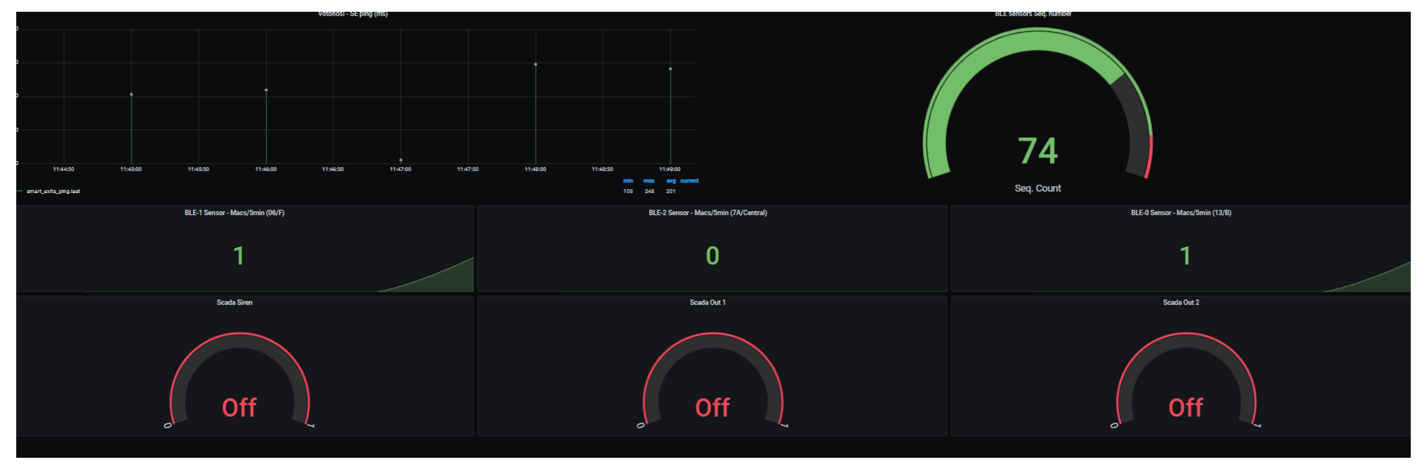
Each of the three Bluetooth and BLE devices scans for advertisement packets continuously and receives the proximity values of the received signal strength indicator (RSSI) from users’ smartphones or vehicles’ Bluetooth devices. Once the scanning process is in progress, the RSSI values are remotely stored in the MongoDB clustered database using the JSON format. Detection results are illustrated in real time by the application service Grafana dashboards. Each Bluetooth detector (dongle) can scan one Bluetooth advertisement channel each time. All the Bluetooth transponders are simultaneously instantiated using three different threads as parts of a single service instance. 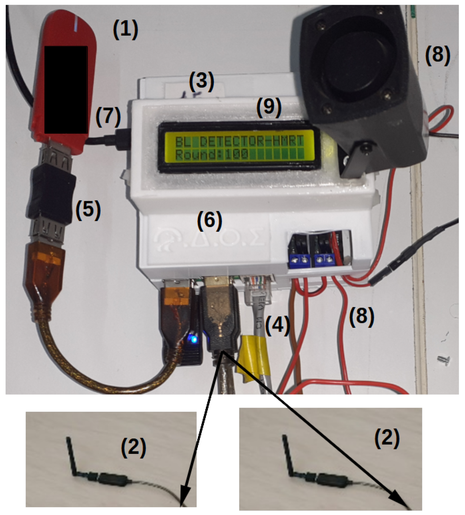Figure 3 depicts the end node BL-detector device implementation [8] and parts, described below:

1.

The USB 4G dongle, which is responsible for the detector’s network connectivity (also an Ethernet port is available for either connectivity or debugging purposes).

2.

The class-1 long range Bluetooth dongles support Bluetooth 3, 4.2 and 5.X protocols and are used to scan active Bluetooth devices. The dongles have high temperature resistance up to 70 ${}^{°}$C and for low temperatures, down to −10 ${}^{°}$C.

3.

BLE dongle adapter that includes a 2 dBi dipole antenna. It is a class-2 adapter embedded in the microcontroller covering the area near the smart exit, with a second USB dongle BLE adapter covering periodically the same area around the tunnel exit.

4.

The Ethernet port, which is used for Ethernet communication and for power over Ethernet (PoE) supply (if applicable).

5.

The USB cable adapter or extender to adjust the USB dongle in a position with better cellular signal reception.

6.

The ABS 3D printed enclosure with the initials of the project printed on the cover.

7.

The main power input via a USB type C cable, if PoE is not available (via the Ethernet cable).

8.

A small speaker, used for issuing sound alerts in case of an emergency and for navigation purposes toward the tunnel exit in cases of limited visibility (fire, or smoke inside the tunnel). It also includes two solid-state relay outputs connecting to the tunnel exit led stripes.

9.

A 16 × 2 Character LCD display, which is used for onsite BL-detector device status information.

The previously presented end-node BL-detector prototype is a technology readiness level 9 (TRL 9) end node device that was successfully tested and validated in its appliance environment. The BL-detector equipment ensures conformity with the EU-wide requirements for operational types of equipment inside tunnels and the local government laws and regulations for wireless transmissions, making it an industry-ready real-time detection implementation.

For the Bluetooth detection process to be quick and accurate, three threaded processes are instantiated, assigned to each of the Bluetooth dongles and one for the two BLE dongles accordingly. Each Bluetooth dongle is assigned to a different advertisement channel per scan interval. Moreover, another threaded dispatched instance per thread is used from the asynchronous threaded pool to send the JSON data to the load balancer and the MongoDB service.

Table 1. Total BL-detector mean scanning time and data recording time using a single MongoDB instance and a load balancing switch that connects to a redundancy clustered MongoDB service.

Load Balancing	Scan Time (ms)	Data Insertion Time (ms)	Total Cycle Time (ms)
Yes	180	212	462
No	180	255	495

presents the results of total Bluetooth scan time, data insertion time, and periodic total cycle time. Using this threaded service approach, the authors managed to reduce the overall scanning process to 180–250 ms. Similarly, the data storing process achieved a maximum of 250–350 ms for all dongle data insertions (maximum entire scanning-recording cycle total time at 660 ms), without the use of the ALBL load balancer, and maximum values of 580–600 ms with the use of the load balancer. The scanning interval for each Bluetooth dongle is 60 ms, which for the class-1 dongles means that they can scan a car driving at a high speed of 200 km/h at least 4–5 times and 7–8 times for a vehicle driving at the speed limit of 130 km/h.

Based on this BL-detector scanning capability, the Friis formula can be used to estimate vehicle distances from the BL-detector dongles and therefore calculate a speed estimation value. Furthermore, since most cars or drivers include in their car an active Bluetooth device, the system can infer speed estimations, or, in the case of tunnel emergencies, if the involved people have their mobile phones, the Bluetooth device set on the system can detect them as instances inside the tunnel or in close proximity to the tunnel’s exit and offer helpful feedback for their release. The following subsection presents the authors’ proposition toward a speed estimator using their BL-detector device that provides better accuracy for the speed of the moving vehicles than using the Friis formula.

3.2. End-Node Speed Estimation and Validation Process

The authors propose a new methodology for estimating speed of moving vehicles in tunnels using a nondeterministic approach. This approach includes a classification engine that uses pre-trained classifiers from RSSI field data and deriving speed category estimations. The authors’ proposition is illustrated in Figure 4.

According to the authors, the speed estimation process is as follows: Instead of using a formula (such as the Friis equation or the use of Friis equation with a pre-filtering Kalman filter step [29]), a different approach is followed. For the distance estimation over time using RSSI values, RSSI values are matched to speed classes (training process), using the output of another system for the actual speed validation, the tunnels’ TMS-IL system. Most contemporary tunnels include inductive loops at their entrances and in front of the tunnels’ escape exits.

Different classifiers can be trained using the BL-detector measurements over time as input and the corresponding measurements from the inductive loops as output. That is, the light GBM (LGBM) [30], the MLP [31], the random forest (RandomForest) [32], the decision tree (DecisionTree) [33], and the extra trees (ExtraTrees) [34] classifiers. The total number of data is 3927, using 20% for testing purposes and the calculation of the accuracy metric. This is because the F-score metric cannot accurately represent the classification accuracy: the recall part of the score leads to low score values (not all IL output measurements have corresponding BL-detector RSSI values), and the precision is merely an indication of the detector’s accuracy.

Prior to classifiers training, appropriate pre-processing data cleansing as well as data impairments compensation must apply. This data pre-processing methodology includes the following pre-processing steps (filtering process):

• Discard data with velocity less than 1 km/h. Explanation: It is only logical that vehicles with a reported speed of less than 1 km/h are due to malfunctions of the TMS-IL system.
• Discard data with velocity over than 220 km/h. Explanation: It is only logical that vehicles with a reported speed of more than 220 km/h are due to malfunctions of the TMS-IL system.
• Discard data with velocity over the 99.6% range from the Gaussian probability distribution. Explanation: The data provided by the TMS-ILs follow the Gaussian probability distribution. As a result, the outliers lie beyond the 99.6% range.
• Discard MAC IDs scanned only from one BLE-detector. Explanation: If a MAC ID that the detectors have scanned is a vehicle, there will be at least one scan from each BL-detector. On the other hand, MAC IDs that are scanned only from one detector are no vehicles passing through the tunnel and are not part of the train dataset.
• Discard MAC IDs for which the total time inside the tunnel is more than the minimum speed times the Bl-detector effective coverage length (21 s). Explanation: The slowest vehicle from the TMS-IL data has a speed of 20 km/h, which converts to 5.555 m/s. The BL-detector’s effective coverage length is 500 m, but the coverage radius range of the Bluetooth class-1 transponders is 50 m. There are two class-1 Bluetooth transponders with 20 m distance between them, so the total range that the BL-detector can scan in an open environment is 120 m. As a result, a vehicle with the slowest speed recorded needs 21.621 s to pass through the active scanning area of the BL-detector.

The post-processing optimization step of the classifiers’ train parameters is achieved through a grid search of their hyperparameters. Using F1 score metric, for the classifiers’ testing process on the 20% of the data of the collected dataset, the most accurate parameters per classifier are detected.

Table 2. Grid test classifiers’ parameters and optimal parameters (in bold), in terms of F1 score.

Algorithm	Hidden Layer Size	Solver	Alpha Value	Learning Rate
MLP	100, 200, 400, 750, 900	lbfgs, sgd, adam	0.1, 0.01, 0.001, 0.0001	constant, invscaling, adaptive
Algorithm	Splitter	Max depth	Criterion	-
DecisionTree	best, random	None, 5, 10, 15, 20, 25, 30, 35, 40, 45	gini, entropy	-
Algorithm	N_estimators	Max depth	Criterion	-
ExtraTrees	100, 200, 400, 500, 600, 800	None, 5, 10, 15, 20, 25, 30, 35, 40, 45	gini, entropy	-
Algorithm	N_estimators	Max depth	Criterion	-
RandomForest	100, 200, 400, 500, 600, 800	None, 5, 10, 15, 20, 25, 30, 35, 40, 45	gini, entropy	-
Algorithm	Boost Type	Max depth	N_leaves	N_estimators
				learning rate
LGBM	gbdt, dart, rf	10, 20, 30, 40, 50	10, 20, 30, 40	100, 200, 400
				0.1, 0.01, 0.001

shows the parameters per classifier put to the test during the grid test, as well as the optimal test parameter outputs per classifier.

For measuring per class accuracy, the authors introduced a new measure called accuracy per class (APC), as an augmented exponential precision calculation function per class, defined as

$$AP{C}_i=\frac{1}{m_{i_{TMS}}}\sum _{l=1}^m(\frac{n+1}{n}·\frac{1}{\frac{1}{n}+2^{k·\left(\right|X{0}_{i_l}-X{1}_{i_l}\left|\right)}})$$

(1)

where i = 1…n are the number of speed classes, $X{0}_i$ is the speed class as calculated by the trained classifier and $X{1}_i$ is the speed class as calculated by the TMS-IL system, for each vehicle l = 1…m detected by the classifier in the class i. The value m is the total number of vehicles detected for that class, and $m_{i_{TMS}}$ is the total number of vehicles detected by the TMS-IL system for that specific class. $k\ge 1,k\in {\mathbb{N}}^{*}$, is a coefficient that exponentially reduces accuracy in cases of $APC>1$. This is, of course, due to the concentration of most of the accurate classified values as well inaccurate ones belonging to a different class of erroneous values. In the authors’ experimentation, the value k is the minimum value, so at least one class has $APC\le 1$, usually $k=[1,3]$.

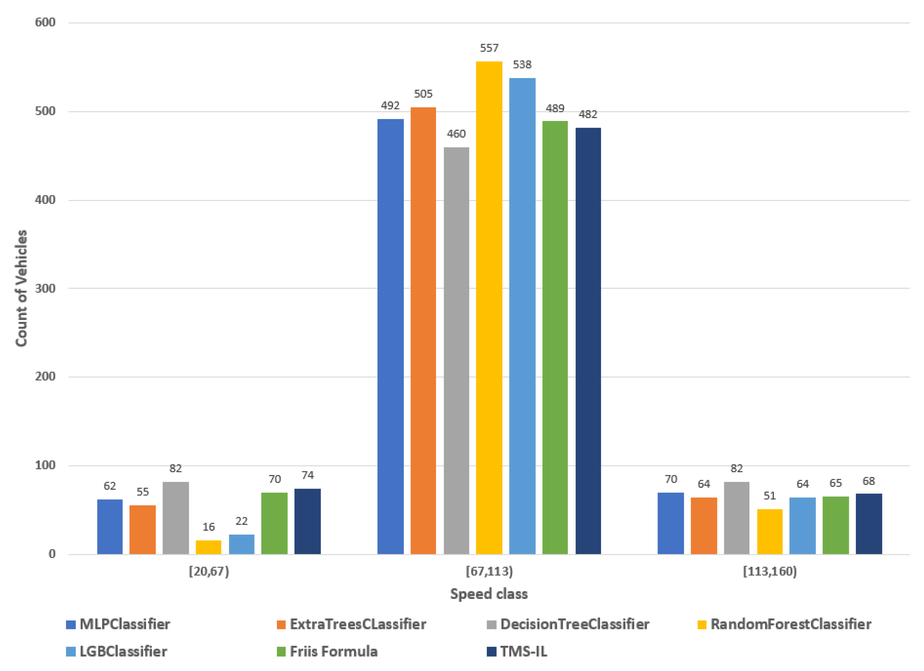
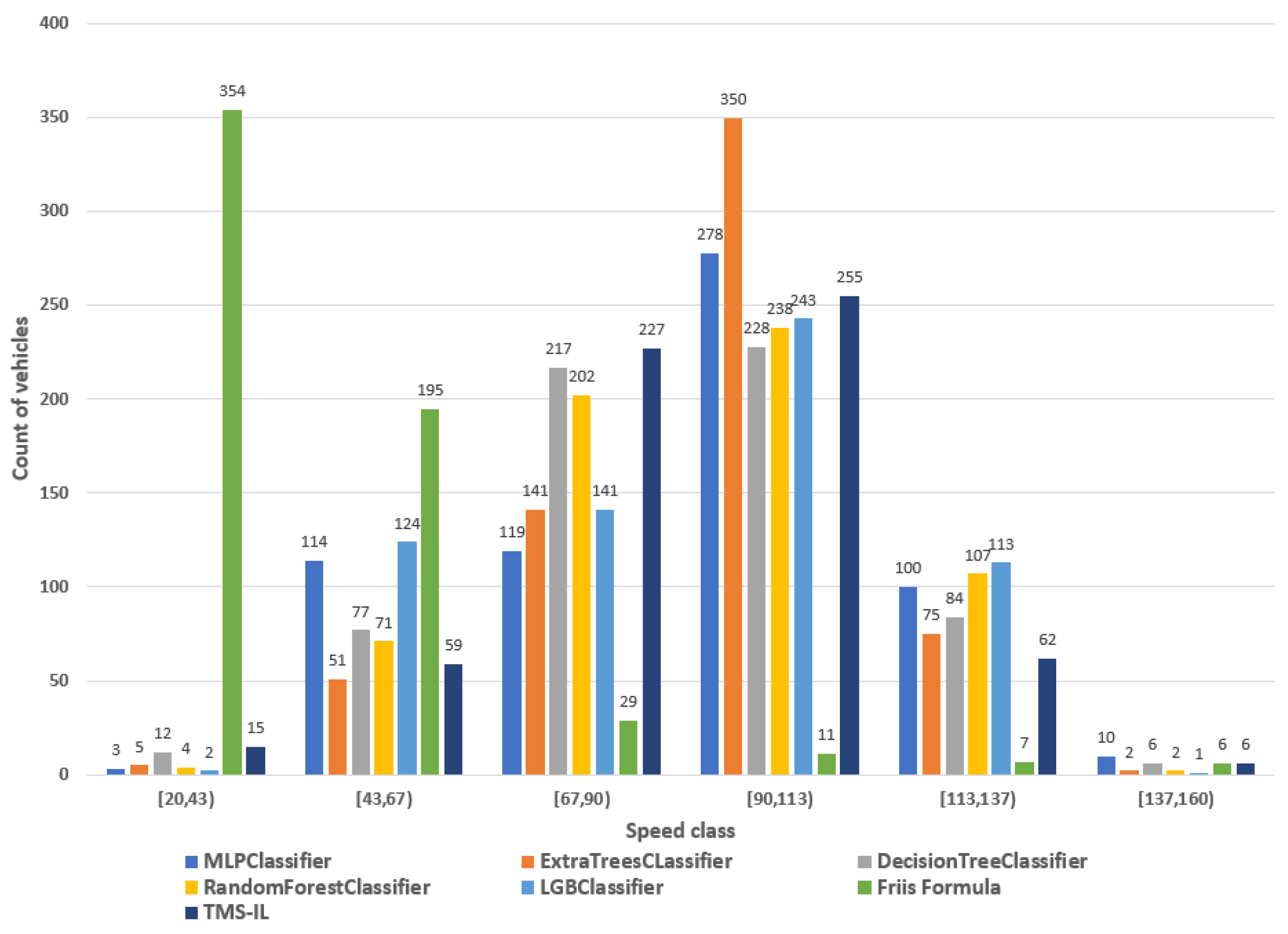
The accuracy per class (APC) is a weighted metric using an exponential formula to deliver balanced weights to vehicles that are misclassified. The purpose of the metric is to add an in-between-classes distance, so the vehicles that are wrongfully distributed can add a weighted bit of precision. Speed classes that are close to each other can provide information regarding the accuracy of the model. It is calculated by the mean $AP{C}_i$ for each class for the vehicles detected from the BL-detector and categorized to the specific class. The mean $AP{C}_i$ calculates the APC of the system separately for all classes and vehicles detected by the BL-detector. There are cases where the total $APC$ value is greater than 1. This means that most of the vehicles detected as well as a significant number of vehicles should not belong to this class. In those cases, the $APC$ value can be set equal to zero, or $APC=\frac{APC}{2·(n+1)}$, where $n\ge 3$ is the total number of classes used. If $APC\le 1$ still, then $APC=0$ for that class.

Regarding Figure 4, an automated pipeline is constructed specifically for the pre- and post-processing steps. Receiving as input the RSSI measurements and the TMS-IL data, which are collected in real time (almost every 500 ms), in the pre-processing step, meaning the data-filtering process, each RSSI datum is assigned to its proper speed class according to the corresponding TMS-IL categorization. Subsequently, concerning the post-processing step, which is mentioned as the training process in Figure 4, once the input data are filtered, the training of each classifier is performed periodically at the time when a dataset will contain data of one month, resulting in a process that is completed in a few milliseconds (for each monthly dataset, per classifier). This automated two-step processing pipeline is compulsory to be repeated every month only until we gather a certain and representative data collection per speed class. A criterion for halting data filtration and classifiers’ retraining, for example, could be the stabilization of the APC accuracy.

Moreover, the automated pipeline process is as follows: RSSI data are collected in real time when Bluetooth transponders are detected. Regarding Figure 4, the real-time data acquired pass through a fully automated pipeline consisting of a pre-processing filtering step and a post-processing training step to achieve speed predictions, similar to [35]. Each Bluetooth detector can acquire more than one RSSI value of each detected Bluetooth MAC. The number of RSSI values/Bluetooth/MAC depends on the users’/vehicles’ moving speed. The BLE devices, which detect vehicles only close to the tunnel exits, require no post-processing or estimation, apart from the appliance of the Friis equation and a pre-processing data cleansing step including impairments compensation. This pre-processing step interval is 500 ms up to 1 min. It is close to the interval for the application service to reload and renew its dashboards. During this time, each detector node retrieves RSSI data as well as TMS-IL output speed data from the MongoDB service, whereas each RSSI datum is assigned to its proper speed class, according to the corresponding TMS-IL categorization. The same pre-processing step applies for the Bluetooth class-1 device, followed by a classifier speed prediction. Subsequently, the post-processing training interval for the estimators training is periodically instantiated in each node every month, resulting in a process which is completed in a few milliseconds (for each monthly dataset, per classifier). During the testing phase, the $APC$ values per class are calculated. The newly trained classifier is used if a $max\left(APC\right)\ge 0.7$ is achieved. If not, it is discarded, and a new training process is scheduled that uses the aggregated data of the two intervals for its next post-processing step. This automated two-step processing pipeline is compulsory to be repeated every month only until we gather a certain and representative data collection per speed class. A criterion for halting data filtration and classifiers’ retraining could be the stabilization of the APC accuracy. In the next section, the authors’ experimentation that includes BL-detector system validation and evaluation of their speed estimation process proposition is presented.

4. Experimental Scenarios and Results

The purpose of this experimentation is to validate BL-detector functionality as well as to evaluate the authors’ prediction velocity model. This is accomplished by using the TMS-IL values as the actual speed output and the Friis Equation (2) speed values for velocity cross-comparison with the trained classifiers estimations. The BLE-detector provides us with data regarding the RSSI (received signal strength indicator) values, the MAC IDs of the Bluetooth devices, and Bluetooth discovery timestamps.

In addition, TMS-IL provides information regarding the current velocity of every vehicle, the type of vehicle based on the induction time length, and the timestamp of the scan. The APC metric is used and calculated both for the Friis speed estimation as well as the classifiers estimations, according to the proposed process in Section 3.2.

4.1. BL-Detector Detection Validation

This experimental scenario compares the measurements taken from the EGNATIA TMS system inductive loop detectors and our BL-detector device. To compute the velocity of the vehicles, the Friss Equation (2) is used.

$$v=\frac{d}{t}=\frac{{10}^{\left(n(P_t-P_d)\right)}}{t}$$

(2)

At first, calibrations of the BL-detector Bluetooth scanners and experimentation to discover the optimal value for the formula n coefficient are performed by cross comparing the results with those taken from the TMS-IL system to attain the best possible tunnel n coefficient ($n=1.2$ for tunnel environment). Consequently, for every RSSI value, a distance estimation from each Bluetooth detector is calculated. To calculate the vehicle’s velocity due to the proximity (20 m) of the two Bluetooth class-1 detectors, we use the following Equation (3):

$$v=\frac{ds}{dt}$$

(3)

where the differences in distance $ds$ and time $dt$ are the differences among two consecutive scans of the same Bluetooth dongle as distinguished by its MAC ID. Every MAC ID is represented using two data series of velocities, one for each Bluetooth class-1 scanner accordingly. Then, the calculation process of the mean speed is performed for each scanner separately. After that, the mean speed of both scanners is calculated so that each Bluetooth MAC ID detected corresponds to one mean velocity value.

To validate the results, every MAC ID’s timestamp and speed value is cross-compared with the timestamps and recorded velocity values from the EGNATIA TMS-IL system. The results are presented in

Table 3. Number of detected vehicles per class.

Class (km/h):	40–50	50–60	60–70	70–80	80–90	90–100	100–110	110–120	120–130	130–140
TMS-IL	54	44	47	66	62	56	58	32	24	9
BL-detector	43	41	46	60	49	32	24	30	23	7

, showing the number of vehicles detected by one of the two BL-detector class-1 transponders, over 10 classes of speed, compared to the measurements taken from the corresponding close to the detector TMS-IL. The presented measurements are taken for one month (March 2021). The data speed measurements calculated by the BL-detector node (Equation (2)) are compared to the calculated speed from TMS-IL system, using as key reference the timestamp of the TMS-IL measurements and an offset value of ±10 s.

According to this experimentation, all BL-detector detected speeds per class are close or below the TMS-IL detected values, even with a less accurate formula such as Equation (2). This is a validation that the BL-detector can detect the vehicle speeds with minimum errors since there are no classes that the detector discovers more vehicles than the TMS-IL system. The fact that it detects fewer vehicles in some classes is irrelevant to the speed estimation. It is affected by the lack of Bluetooth devices at these vehicles to be discovered by the BL-detector.

4.2. Evaluation of the BL-Detector Speed Classification Process

This experimentation scenario investigates different classifiers used by the proposed classification process with the Friis formula. The output given from the TMS-IL system is used as the ground truth.

To create a model that predicts the velocity of incoming vehicles from the RSSI values, the authors linked vehicles from TMS-IL detector to MAC IDs using the timestamp of the scans. Because the TMS-IL detectors are in the middle of the tunnel, the difference in time of the scans must be less than or equal to 10 s, and they can be no other scan of different MAC IDs from the BLE-detectors for another 21 s. Considering these values, the authors trained their classifiers using input and output taken from the Votonosi tunnel BL-detector for three months (June 2021–August 2021). To continue, including the data taken from September 2021, the authors evaluated their model and compared the classifiers’ output with both the Friis equation output and the TMS-IL output, in terms of number of vehicles detected per class, as well as $APC$ accuracy per class.

The evaluation of the proposed classification process was initialized by maintaining 3, 4, 6, and 8 classes. Therefore, the per-class detected and countenanced vehicles was calculated for each of those classes and the $APC$ accuracy per class. The following classifiers were used toward the classification process: the light GBM [30], MLP [31], random forest [32], decision tree [33], extra trees [34] classifiers and the Friis Equation (2). The results of the number of vehicles for classes 3, 4, 6, and 8 and the results of accuracy in terms of $APC$ are presented in the following subsections.

Experimentation Using 3-Classes

In this experimental case, the authors used three classes of speed, experimenting with different classifiers. Figure 5 illustrates the number of vehicles classification for each classifier to each class, while

Table 4. The 3-classes—classifiers ranking. Total $APC$ per class and Friis equation total $APC$.

APC/Alg.—km/h:	20–66	67–102	103–160
Friis Eq.	0.90	0.97	0.91
MLP	0.80	0.97	0.98
ExtraTrees	0.70	0.96	0.89
DecisionTree	0.75	0.64	0.82
LGBM	0.24	0.91	0.77
RandomForest	0.17	0.94	0.61

presents the $APC$ values achieved per class per classifier.

5. Vehicles Count per Trained Classifier and Friis Formula over TMS-IL System Count

For the 3-classes classification case (low, medium, high speeds), the results in Figure 5 show that all classifiers follow the TMS-IL detection, and all, except decision tree, detect more vehicles than the TMS-IL for medium speeds and fewer vehicles for low and high speeds. The decision tree behaves inversely, detecting more vehicles at the medium speed class.

Comparing the Friis equation with classifiers, the $APC$ results in Table 4 show that the MLP classifier and Friis equation present similar performance results for a small number of classes and outperform all other classifiers. Comparing Friis and MLP, MLP performs better for a medium speed, while the Friis formula outperforms MLP for both low and high speeds. Observing Table 4, it is apparent that all classifiers have $APC$ values above 70%, set as the acceptance criteria from the authors’ classifications process, except the random forest and LGBM classifiers. The decision tree and extra trees classifiers also maintain above 70% classification accuracy results in terms of $APC$, which means that these algorithms, along with Friis and MLP, can be selected as detection classifiers according to the authors’ classification process.

5.1. Experimentation Using 4-Classes

In this experimental case, four classes of speed were selected, experimenting with different classifiers. Figure 6 illustrates the number of classified vehicles per classifier to each class, while

Table 5. The 4-classes—Classifiers ranking. Total $APC$ per class and Friis equation total $APC$.

APC/Alg.—km/h:	20–54	55–89	90–124	125–160
DecisionTree	0.86	0.41	0.59	0.55
MLP	0.33	0.72	0.72	0.30
Friis Eq.	0.75	0.29	0.68	0.34
ExtraTrees	0.31	0.46	0.64	0.12
RandomForest	0.16	0.41	0.71	0.09
LGBM	0.18	0.40	0.60	0.01

presents the $APC$ values achieved per class per classifier.

For the 4-classes classification case, the obtained results depicted in Figure 6 show that the Friis equation can detect all the vehicles for low and high-speed classes. Nevertheless, it erroneously detects most of the vehicles to the low-speed class, which in turn diminishes the Friis $APC$ as shown in Table 5. The Friis equation cannot discriminate among classes of medium speeds, but it can accurately detect low- and high-speed classes. From all the other classifiers, none can achieve more than 70% $APC$ values (see Table 5), which means that more training data are required to provide accurate results. The decision tree classifier maintains a low 17% decrease in its $APC$ value, while the random forest classifier presents a 37% increase in its $APC$ value. However, 20% less than the decision tree value and 10% less than the MLP value is achieved.

5.2. Experimentation Using 6-Classes

In this experimental case, six classes of speed were determined, experimenting with different classifiers. Figure 7 illustrates the number of classified vehicles per classifier to each class, while

Table 6. The 6-classes—Classifiers ranking. Total $APC$ per class and Friis equation total $APC$.

APC/Alg.—km/h:	20–42	43–66	67–89	90–112	113–136	137–160
DecisionTree	0.57	0.30	0.86	0.90	0.33	0.28
RandomForest	0.19	0.28	0.80	0.94	0.42	0.09
LGBM	0.09	0.49	0.56	0.96	0.44	0.04
Friis Eq.	0	0.77	0.11	0.52	0.33	0.28
MLP	0.14	0.11	0.37	0.77	0.09	0.09
ExtraTrees	0.23	0.20	0.56	0.01	0.29	0.09

presents the $APC$ values achieved per class per classifier.

For the 6-classes classification case, the derived results are shown in Figure 7 pinpointing that Friis misclassifies most of the vehicles to the low-speed classes and extra trees for the class [90–113] km/h, followed by the MLP classifier. Both classifiers present worse results than the Friis equation in terms of total $APC$ as shown in Table 6. The Friis equation successfully detects all the vehicles from classes [20–43] km/h and [137–160] km/h. However, due to the fact that it cannot easily discriminate vehicles to other classes and infers that most of the vehicles are of the 1st class, it has an $APC=0$ for that class (see Table 6).

Decision tree, random forest, and light GBM manage to maintain $APC$ values above 40%, with decision tree having the maximum mean $APC$ value of 54.41%, followed by random forest. It is also important to notice that for classes of [67–112] km/h, where most of the vehicles reside according to TMS-IL, decision tree and random forest provide increased $APC$ results with accuracies above 80%. The same applies to the MLP classifier for class [90–112] km/h. Increasing the number of observations per class in the training dataset will increase the classification accuracy.

5.3. Experimentation Using Eight Classes

In this experimental case, the authors used eight classes of speed, experimenting with different classifiers. Figure 8 illustrates the number of classified vehicles for each classifier to each class, while

Table 7. The 8-classes—Classifiers ranking. Total $APC$ per class and Friis equation total $APC$.

APC/Alg.—km/h:	20–37	38–54	55–71	72–89	90–107	108–124	125–141	142–160
DecisionTree	0.21	0.88	0.75	0.61	0.58	0.64	0.2	0.06
LGBM	0.05	0.31	0.57	0.7	0.90	0.35	0.28	0.19
RandomForest	0.1	0.27	0.15	0.93	0.65	0.22	0.23	0.37
ExtraTrees	0.16	0.27	0.22	0.06	0.64	0.32	0.19	0.35
Friis Eq.	0	0.15	0.51	0.29	0.03	0.02	0.28	0.30
MLP	0.02	0.36	0.02	0.67	0.06	0.09	0.68	0.04

presents the $APC$ values achieved per class per classifier.

For the 8-classes classification case, Friis and MLP present the worst total $APC$ values (see Table 7), close to 25%. Friis has most of its values at classes [20–35] and [38–55] km/h, as shown in Figure 8. Similarly, as shown in Table 7, random forest and extra trees present similar accuracy values of less than 40%. Light GBM and decision tree maintain the maximum $APC$ values, with the decision tree outperforming light GBM by 15%. MLP and extra trees do not provide good accuracy results, and in most classes, Friis outperforms them. In addition, Friis presents above 70% accuracy results for the high-speed class and detects all vehicles for the low-speed class. Nevertheless, the misclassification of most of the speed results to the lowest class remains, thus having an $APC=0$.

5.4. Results Summary

Examining the above scenario cases, it is obvious that the Friis equation can be used for low-speed classes (up to 20 km/h). It can also achieve similar high $APC$ values for high-speed classes (above 120 km/h). Since this is the case, prior to classification or for the BLE device of the BL-detector, the Friis equation can be used to detect stranded people inside tunnels in cases of emergency (smoke or fire).

Table 8. Summary table of classifiers’ accuracy ranking, based on $APC$, for different speed classes (3, 4, 6, 8).

No Classes:	3 Classes	4 Classes	6 Classes	8 Classes
Selected Classifiers
DecisionTree	74.08%	60.91%	54.41%	49.97%
LGBM	64.36%	33.43%	43.49%	42.45%
RandomForest	34.68%	48.71%	45.68%	36.84%
ExtraTrees	85.46%	38.85%	23.23%	27.97%
MLP	92.41%	52.20%	26.79%	24.26%
Friis Eq.	93.32%	34.54%	33.89%	25.22%

summarizes the mean accuracy recults taken from all classifiers for 3, 4, 6 and 8 classes accordingly.

The authors confirm their classification process by showing that in all cases (see Table 8), a classifier can outperform the Friis equation and provide better accuracy if the classifiers are successfully trained through a data-filtering supervised process, as proposed. They also pinpoint that doubling the data for the training process up to six classes of speed will increase the classifier’s accuracy above 70% for classes above 40 km/h and less than 120 km/h.

According to Table 8, the decision tree classifier presents the best accuracy, maintaining above 50% accuracy in all cases, with minimum variations per class, followed by light GBM and random forest. So in most cases, a tree-based classifier can provide robust classification results, even with low data. The Friis equation is still the preferred option for extremely low datasets or classes with limited data (speeds below 20 km/h or above 160 km/h). The authors set future data acquisition, especially for speeds below 20 km/h, which accurately represent people’s mobility inside tunnels.

Finally, detected variability of the APC among classes is because the amount of data for the medium-speed classes is larger compared to low- or high-speed classes (to support this claim, EU regulations forbid low- and high-speed vehicle movements inside tunnels). As a result, the classifiers cannot acquire sufficient data to be trained correctly, due to the lack of RSSI and TMS-IL measurements. The authors set the better evaluation and training of their proposed classifiers for low- and high-speed classes as future work.

6. Conclusions

This paper presents a scaleable and distributed crowd-sensing Bluetooth system, called BL-detector, and proposes a speed estimation process for vehicles using trained classifiers. The proposed system functionality is based on a prototype BL-detector node with multiple Bluetooth long-range and BLE short-range transceivers. The proposed system achieves (a) the MIMO characteristics and AoA/AoD functionality of Bluetooth 5.2 and (b) long-range coverage area, ten times bigger than the coverage area of a BLE device. Furthermore, the system has been implemented to sense people and vehicles moving inside the motorway tunnels exits.

The proposed system can also trigger alerts since it is placed above the tunnel exits and interfaces with the motorway resources management system, which includes outputs connecting with audio and visual actuators, such as loud spouts and LED stripes in proximity to the tunnel exits.

Moreover, it can detect people in proximity and calculate the speed of passing vehicles. Finally, focusing on speed accuracy, the authors noticed that the Friis equation for speed estimations fail to provide accurate results, introducing variations due to the tunnel environment. For this reason, the authors proposed a new speed calculation process that utilizes the most accurate trained classifier, under supervised learning from another motorway system called TMS-IL, installed at the tunnel openings and used for detecting speed movements using classes of speed.

The evaluation process using classifiers has shown that the decision tree and random forest classifiers manage to present significant detection results of above 35% and 50% accuracy, accordingly. For several classes (above 8) and low, the Friis accuracy is less than 25%. Below 20 km/h and above 120 km/h, where the data are limited, the Friis formula can detect speed with a maximum accuracy of less than 35%. At the same time, all other classifiers fail to detect more than 20%. Furthermore, algorithms such as decision tree, random forest, and light GBM outperformed the Friis formula by achieving mean accuracies up to 77% in classes where vehicle data are primarily concentrated. The authors also noticed that the limited accuracy of their classification process was due to the shortage of data (3 months of data) and pinpointed that their accuracy will further increase another 7–12% when their trained dataset doubles in terms of observations. Therefore, the authors confirmed the functionality of their proposed system and their classification process’ capability of providing accurate results; they set the evaluation of their system with a new trained dataset and the deployment of more BL-detector end nodes as future work.

References

1. Bai, J.; Liao, H.; Xia, Y. Study on Fire Accidents in Tunnels. IOP Conf. Ser. Mater. Sci. Eng. 2020, 1, 171–177. [Google Scholar] [CrossRef]
2. Kirytopoulos, K.; Dermitzakis, E.; Ntzeremes, P.; Chatzistelios, G. Holistic Management of Risks for Road Tunnels. In Proceedings of the 13th International Conference on Modeling, Optimization and Simulation—MOSIM’20, Agadir, Morocco, 12–14 November 2020. [Google Scholar]
3. Ren, R.; Zhou, H.; Hu, Z.; He, S.; Wang, X. Statistical analysis of fire accidents in Chinese highway tunnels 2000–2016. Tunn. Undergr. Space Technol. 2019, 83, 452–460. [Google Scholar] [CrossRef]
4. Ntzeremes, P.; Kirytopoulos, K. Evaluating the role of risk assessment for road tunnel fire safety: A comparative review within the EU. J. Traffic Transp. Eng. (Engl. Ed.) 2019, 6, 282–296. [Google Scholar] [CrossRef]
5. Kirytopoulos, K.; Konstandinidou, M.; Nivolianitou, Z.; Kazaras, K. Embedding the human factor in road tunnel risk analysis. Process Saf. Environ. Prot. 2014, 92, 329–337. [Google Scholar] [CrossRef]
6. Król, A.; Król, M. The factors determining the number of the endangered people in a case of fire in a road tunnel. Fire Saf. J. 2020, 111, 102942. [Google Scholar] [CrossRef]
7. Ntzeremes, P.; Kirytopoulos, K. Applying a stochastic-based approach for developing a quantitative risk assessment method on the fire safety of underground road tunnels. Tunn. Undergr. Space Technol. 2018, 81, 619–631. [Google Scholar] [CrossRef]
8. Asiminidis, C.; Kokkonis, G.; Kontogiannis, S. BLE Sniffing for Crowd Sensing and Directionality Scanning of Mobile Devices Inside Tunnels. In Proceedings of the 2020 3rd World Symposium on Communication Engineering (WSCE), Thessaloniki, Greece, 9–11 October 2020; pp. 54–58. [Google Scholar] [CrossRef]
9. Lee, B.; Han, D. Real-Time Fire Detection Using Camera Sequence Image in Tunnel Environment. In Advanced Intelligent Computing Theories and Applications. With Aspects of Theoretical and Methodological Issues; Huang, D.S., Heutte, L., Loog, M., Eds.; Springer: Berlin/Heidelberg, Germany, 2007; pp. 1209–1220. [Google Scholar]
10. Yan, B.; Li, J.; Zhang, M.; Zhang, J.; Qiao, L.; Wang, T. Raman Distributed Temperature Sensor with Optical Dynamic Difference Compensation and Visual Localization Technology for Tunnel Fire Detection. Sensors 2019, 19, 2320. [Google Scholar] [CrossRef] [Green Version]
11. Aralt, T.; Nilsen, A. Automatic fire detection in road traffic tunnels. Tunn. Undergr. Space Technol. 2009, 24, 75–83. [Google Scholar] [CrossRef]
12. Xiqiang, W.; Park, Y.; Ao, L.; Huang, X.; Xiao, F.; Usmani, A. Smart Detection of Fire Source in Tunnel Based on the Numerical Database and Artificial Intelligence. Fire Technol. 2020, 57, 657–682. [Google Scholar] [CrossRef]
13. Kamijo, S.; Fujimura, K. Incident Detection in Heavy Traffics in Tunnels by the Interlayer Feedback Algorithm. Int. J. Intell. Transp. Syst. Res. 2010, 8, 121–130. [Google Scholar] [CrossRef] [Green Version]
14. Sarvari, A.; Mazinani, S.M. A new tunnel fire detection and suppression system based on camera image processing and water mist jet fans. Heliyon 2019, 5, e01879. [Google Scholar] [CrossRef] [PubMed] [Green Version]
15. Sisias, G.; Kontogiannis, S.; Konstandinidou, M.; Dossis, M. Preliminary results of a proposed CNN framework for use in motorway applicable detection systems. In Proceedings of the 2020 5th South-East Europe Design Automation, Computer Engineering, Computer Networks and Social Media Conference (SEEDA-CECNSM), Virtual Event, 25–27 September 2020; IEEE: Piscataway, NJ, USA, 2020; pp. 1–7. [Google Scholar] [CrossRef]
16. Konstantinidou, M.; Sissias, G.; Kontogiannis, S. Development of a Proactive Tool for Dangerous Goods Management in Tunnels. In Proceedings of the 31st European Safety and Reliability Conference—ESREL, Angers, France, 19–23 September 2021; Volume 1. [Google Scholar] [CrossRef]
17. Gomez, C.; Oller, J.; Paradells, J. Overview and Evaluation of Bluetooth Low Energy: An Emerging Low-Power Wireless Technology. Sensors 2012, 12, 11734–11753. [Google Scholar] [CrossRef]
18. Monfared, S.; Nguyen, T.H.; Petrillo, L.; De Doncker, P.; Horlin, F. Experimental Demonstration of BLE Transmitter Positioning Based on AOA Estimation. In Proceedings of the 2018 IEEE 29th Annual International Symposium on Personal, Indoor and Mobile Radio Communications (PIMRC), Bologna, Italy, 9–12 September 2018; pp. 856–859. [Google Scholar] [CrossRef] [Green Version]
19. Huang, C.; Zhuang, Y.; Liu, H.; Li, J.; Wang, W. A Performance Evaluation Framework for Direction Finding Using BLE AoA/AoD Receivers. IEEE Internet Things J. 2021, 8, 3331–3345. [Google Scholar] [CrossRef]
20. Kolakowski, M.; Djaja-Josko, V. TDOA-TWR based positioning algorithm for UWB localization system. In Proceedings of the 2016 21st International Conference on Microwave, Radar and Wireless Communications (MIKON), Krakow, Poland, 9–11 May 2016; IEEE: Piscataway, NJ, USA, 2016; pp. 1–4. [Google Scholar] [CrossRef]
21. Barua, B.; Kandil, N.; Hakem, N. On performance study of TWR UWB ranging in underground mine. In Proceedings of the 2018 Sixth International Conference on Digital Information, Networking, and Wireless Communications (DINWC), Beirut, Lebanon, 25–27 April 2018; pp. 28–31. [Google Scholar] [CrossRef]
22. Sarkar, S.; Liu, J.; Jovanov, E. A Robust Algorithm for Sniffing BLE Long-Lived Connections in Real-Time. arXiv 2019, arXiv:1907.12782. [Google Scholar]
23. Kontogiannis, S.; Asiminidis, C. Proposed Management System and Response Estimation Algorithm for Motorway Incidents. Energies 2021, 14, 2736. [Google Scholar] [CrossRef]
24. Kontogiannis, S.; Karakos, A. ALBL: An adaptive load balancing algorithm for distributed web systems. Int. J. Commun. Netw. Distrib. Syst. 2014, 13, 144–168. [Google Scholar] [CrossRef]
25. Bradshaw, S.; Brazil, E.; Chodorow, K. MongoDB: The Definitive Guide: Powerful and Scalable Data Storage; O’Reilly Media: Farnham, UK, 2019. [Google Scholar]
26. Asiminidis, C.; Kokkonis, G.; Kontogiannis, S. Database Systems Performance Evaluation for IoT Applications. Int. J. Database Manag. Syst.-IJDMS 2018, 10, 1–14. [Google Scholar] [CrossRef]
27. Chan, N. A Resource Utilization Analytics Platform Using Grafana and Telegraf for the Savio Supercluster. In Proceedings of the Practice and Experience in Advanced Research Computing on Rise of the Machines (Learning), Chicago, IL, USA, 28 July–1 August 2019; Association for Computing Machinery: New York, NY, USA, 2019. PEARC ’19. [Google Scholar] [CrossRef]
28. Grafana Labs. Grafana Documentation. 2020. Available online: https://grafana.com/docs/grafana/latest/ (accessed on 15 July 2019).
29. Yim, J.; Jeong, S.; Gwon, K.; Joo, J. Improvement of Kalman filters for WLAN based indoor tracking. Expert Syst. Appl. 2010, 37, 426–433. [Google Scholar] [CrossRef]
30. Saha, M.; Nayak, S.; Mohanty, N.; Baral, V.; Rout, I. Preterm Delivery Prediction Using Gradient Boosting Algorithms. In Communication and Intelligent Systems; Sharma, H., Gupta, M.K., Tomar, G.S., Lipo, W., Eds.; Springer: Singapore, 2021; pp. 59–68. [Google Scholar]
31. Windeatt, T. Ensemble MLP Classifier Design. In Computational Intelligence Paradigms: Innovative Applications; Springer: Berlin/Heidelberg, Germany, 2008; pp. 133–147. [Google Scholar] [CrossRef]
32. Pal, M. Random forest classifier for remote sensing classification. Int. J. Remote Sens. 2005, 26, 217–222. [Google Scholar] [CrossRef]
33. Safavian, S.; Landgrebe, D. A survey of decision tree classifier methodology. IEEE Trans. Syst. Man Cybern. 1991, 21, 660–674. [Google Scholar] [CrossRef] [Green Version]
34. Alsariera, Y.A.; Adeyemo, V.E.; Balogun, A.O.; Alazzawi, A.K. AI Meta-Learners and Extra-Trees Algorithm for the Detection of Phishing Websites. IEEE Access 2020, 8, 142532–142542. [Google Scholar] [CrossRef]
35. Haider, A.; Wei, Y.; Liu, S.; Hwang, S.H. Pre- and Post-Processing Algorithms with Deep Learning Classifier for Wi-Fi Fingerprint-Based Indoor Positioning. Electronics 2019, 8, 195. [Google Scholar] [CrossRef] [Green Version]
Figure 1. BL-detection system high-level architecture.
Electronics 11 00265 g001
Figure 2. BL-detector real-time detection visualization web view.
Electronics 11 00265 g002
Figure 3. BL-detector end node device prototype and detector enumerated hardware parts.
Electronics 11 00265 g003
Figure 4. Proposed speed estimation–classification process.
Electronics 11 00265 g004
Figure 5. The 3-classes vehicle count per class over TMS-IL count per class.
Electronics 11 00265 g005
Figure 6. The 4-classes vehicle count per class over TMS-IL count per class.
Electronics 11 00265 g006
Figure 7. The 6-classes vehicle count per class over TMS-IL count per class.
Electronics 11 00265 g007
Figure 8. The 8-classes vehicle count per class over TMS-IL count per class.
Electronics 11 00265 g008