A Lightweight Learning Method for Stochastic Configuration Networks Using Non-Inverse Solution

Abstract

Stochastic configuration networks (SCNs) face time-consuming issues when dealing with complex modeling tasks that usually require a mass of hidden nodes to build an enormous network. An important reason behind this issue is that SCNs always employ the Moore–Penrose generalized inverse method with high complexity to update the output weights in each increment. To tackle this problem, this paper proposes a lightweight SCNs, called L-SCNs. First, to avoid using the Moore–Penrose generalized inverse method, a positive definite equation is proposed to replace the over-determined equation, and the consistency of their solution is proved. Then, to reduce the complexity of calculating the output weight, a low complexity method based on Cholesky decomposition is proposed. The experimental results based on both the benchmark function approximation and real-world problems including regression and classification applications show that L-SCNs are sufficiently lightweight.

1. Introduction

Although the deep neural networks have proven to be a powerful learning tool, most networks suffer from time-consuming training due to the massive hyperparameters and complex structures. In many heterogeneous data analytics tasks, flattened networks can achieve promising performance. In the flattened networks, single-hidden layer feedforward neural networks (SLFNs) [1,2] have been widely applied because of their universal approximation capability and simple construction. However, gradient-descent-based learning algorithms are generally adopted for SLFNs training. Therefore, slow convergence and trap in a local minimum are often-encountered problems [3].

The randomized learning method offers a different learning method for flattened networks training. Many randomized flattened networks have been shown to approximate continuous functions on compact sets, and they also have the property of fast learning [4,5]. Stochastic configuration networks (SCNs) [6] provide a state-of-the-art randomized incremental learning method for SLFNs. In comparison with the traditional randomized incremental learning models, SCNs have some advantages: (1) SCNs randomly assign the input weights and biases of the hidden nodes in dynamically adjustable scopes according to the supervisory mechanism; (2) a more compact network structure. Therefore, SCNs have been extensively studied and become a hot topic of neural computing.

For large-scale data analytics, an ensemble learning method for quickly disassociating heterogeneous neurons was proposed is designed for SCNs by using a negative correlation learning strategy [7]. To improve learning efficiency, SCNs with block increments and variable increments are developed, which allow multiple hidden nodes to be added at each iteration [8,9]. Then, point and block increments are integrated into the parallel SCNs (PSCNs) [10]. To resolving the modeling tasks of uncertain data, robust SCN (RSCNs) is proposed by using maximum correlation entropy criterion (MCC) and kernel density estimation [10,11,12]. In order to further improve the expressiveness, SCNs with deep and stacked structures are proposed [13,14,15]. In [16], a two-dimensional SCNs (2DSCNs) is constructed for image data analytics. To address prediction interval estimation problems, the corresponding deep, ensemble, robust, and sparse versions of SCNs were developed [17,18,19]. In addition to the above theoretical studies, SCNs have successful applications in many fields, such as optical fiber pre-warning system [20], industrial process [21], concrete defect recognition [22], and so on.

However, the SCNs construction process can be extremely time-consuming when dealing with complex modeling tasks. The fundamental reason for this is that singular value decomposition (SVD) is needed to solve the output weights [23]. Concretely, the number of rows of the hidden layer output matrix is always much larger than the number of columns [24,25], which makes the hidden layer output matrix to become an over-determined matrix with no inverse [26]. To obtain the output weights, it is necessary to employ SVD to solve Moore–Penrose (M–P) generalized inverse in an over-determined matrix. Theoretically, the complexity of SVD is related with third power of the number of hidden nodes and the product of number of hidden nodes and input dimension. This makes the modeling process of SCNs extremely time-consuming when dealing with complex tasks that require a large network structure (a large number of hidden nodes) to enhance the expressive power of the model.

This paper proposes a lightweight non-inverse solution method for the output weights of SCNs (L-SCNs) by introducing normal equation theory [27] and Cholesky decomposition [28]. The main contributions of the paper are as follows:

• To avoid adopting M–P generalized inverse with SVD, a positive definite equation for solving output weights is established based on normal equation theory to replace the over-determined equation;
• The consistency of the solutions of the positive definite equation and the over-determined equation in calculating the output weights is proved;
• A low complexity method for solving the positive definite equations based on Cholesky decomposition is proposed.

Experimental results on both the benchmark function approximation and real-world problems including regression and classification applications show that, compared with SCNs and IRVFLNs (an incremental variant of RVFLNs), the proposed L-SCNs have a superior performance in lightweight aspect.

The remaining parts of the paper are organized as follows. In Section 2, the basic principle of SCNs and some remarks are shown. The algorithm description of L-SCNs and full proof of related theories are presented in Section 3. In Section 4, the experimental setup is given and the performance of L-SCNs is fully discussed. Some conclusions are drawn in Section 5.

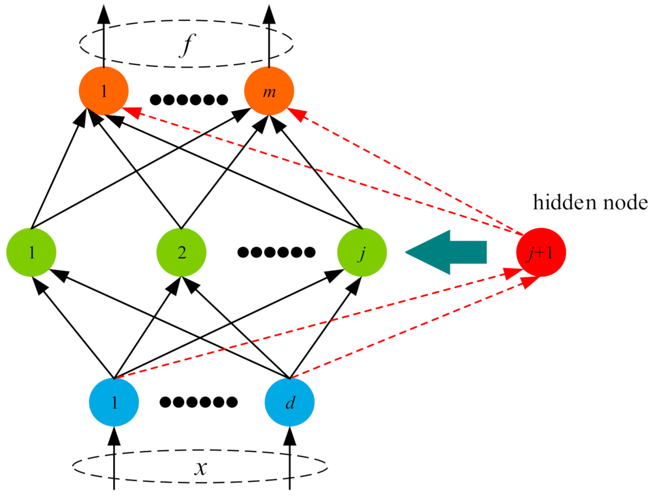
2. Brief Review of SCNs

As a kind of flattened network, SCNs model includes an input layer, hidden layer and output layer. Its hidden layer is constructed incrementally according to the supervisory mechanism. The specific SCNs network structure is shown in Figure 1.

The construction process of SCNs is briefly described as follows:

Given an input $X=\left\{x_1,x_2,\dots ,x_N\right\}$, $x_i\in {ℝ}^d$ and its corresponding output $f=\left\{f_1,f_2,\dots ,f_N\right\}$, $f_i\in {ℝ}^m$. Suppose that we have already built a SCNs with L−1 hidden nodes, i.e.,:

$$f_{L-1}\left(x\right)={\displaystyle {\sum }_{j=1}^{L-1}{\beta }_j^{}}{g}_j\left(w_j^{\mathrm{T}}x+b_j\right)$$

(1)

where ${\beta }_j={\left[{\beta }_{j,1},{\beta }_{j,2},\dots ,{\beta }_{j,m}\right]}^{\mathrm{T}}$ is the output weights vector of the j-th hidden node, $w_j$ is the input weight vector of the j-th hidden node. $b_j$ is the threshold of the j-th hidden node. $g_j\left(w_j^{\mathrm{T}}x+b_j\right)$ is the hidden layer output vector of the j-th node, “$\mathrm{T}$” represents a transpose of the matrix.

The current residual error of SCNs is calculated by Equation (2):

$$e_{L-1}=f-f_{L-1}$$

(2)

The acceptable tolerance error, denoted as ε. If e_L−1 does not reach ε, continue to add new nodes to the SCNs by the supervision configuration mechanism:

$${\xi }_L={\displaystyle {\sum }_{q=1}^m{\xi }_{L,q}}\ge 0$$

(3)

and

$${\xi }_{L,q}=\frac{{〈e_{L-1,q}^{\mathrm{T}}\cdot h_L〉}^2}{h_L^T\cdot h_L}-\left(1-r-{\mu }_L\right){‖e_{L-1,q}^{\mathrm{T}}‖}^2,q=1,2,\dots ,m$$

(4)

where 0 < r < 1 indicates regularization parameter, $\left\{{\mu }_L\right\}$ is a nonnegative real number sequence with ${\mu }_L\le 1-r$ and ${\lim }_{L\to \infty }{\mu }_L=0$, $h_L={\left[g_L\left(w_L^{\mathrm{T}}{x}_1+b_L\right),\dots ,g_L\left(w_L^{\mathrm{T}}{x}_N+b_L\right)\right]}^{\mathrm{T}}$.

The best hidden node parameters are determined by the maximum ${\xi }_L$. Then, the output weights can be evaluated by Equation (5):

$${\beta }^{\ast }=H_L^{†}f$$

(5)

where ${\beta }^{\ast }=\left[{\beta }_1^{\ast },\dots ,{\beta }_L^{\ast }\right]$. $H_L=\left[h_1,\dots ,h_L\right]$ is the current hidden layer output matrix, $h_p=g_p$, $p=1,\dots ,L$. $H_L^{†}$ is M–P generalized inverse matrix of $H_L$.

The above process will be repeated until the residual error reach expected a tolerance $\epsilon$ or hidden nodes reaches the maximum.

Remark 1.

It can be seen that the hidden nodes of SCNs are built incrementally, and all output weights need to be recalculated after each hidden node is added. Therefore, the complexity of the modeling process depends on the evaluation method of the output weights.

Remark 2.

It can be seen from the above analysis,$H_L$is an over-determined matrix. Therefore, M–P generalized inverse method is used to solve the over-determined equation$H_L\beta =f$. However, the complexity of M–P generalized inverse method is related with third power of the number of hidden nodes and the product of number of hidden nodes and input dimension due to the use of singular value decomposition (SVD). Thus, the M–P method is very time-consuming, especially when dealing with complex modeling tasks that require a large number of hidden nodes. In addition, the M–P generalized inverse method can only obtain the approximate solution of the output weights, which is difficult to make the model optimal.

3. L-SCNs Method

From the above analysis, it can be seen that the M–P generalized inverse method involving SVD is the main reason for time-consuming nature of SCNs modeling. In order to solve this problem, a positive definite equation based on normal equation is proposed to replace the over-determined equation. Then, a low computational complexity method based on Cholesky decomposition is proposed to solve the positive definite equation and obtain the output weight, thereby reducing the modeling complexity of SCNs.

3.1. Positive Definite Equation

For the sake of brevity, this paper introduces H to replace H_L. According to normal equation theory, $H\beta =f$ can be denoted by

$$H^{T}H\beta =H^{T}f$$

(6)

Theorem 1 can guarantee the consistency of the solution of positive definite equation and over-determined equation, and a strict proof is given.

Theorem 1.

The necessary and sufficient condition for β* is the least square solution of$H\beta =f$: β* is the solution of$\left(H^{T}H\right)\beta =H^{T}f$.

Proof. 

Sufficiency: Suppose an N-dimensional vector β* such that $\left(H^{T}H\right)\beta =H^{T}f$, given any n-dimensional vector β, $\beta \ne {\beta }^{\ast }$. Let $y=\beta -{\beta }^{\ast }$, $y\ne 0$, so.

$$\begin{array}{l}{‖f-H\beta ‖}_2^2\\ ={‖f-H{\beta }^{\ast }-Hy‖}_2^2\\ =\left(f-H{\beta }^{\ast }-Hy,f-H{\beta }^{\ast }-Hy\right)\\ =\left(f-H{\beta }^{\ast },f-H{\beta }^{\ast }\right)-2\left(Hy,f-H{\beta }^{\ast }\right)+\left(Hy,Hy\right)\\ ={‖f-H{\beta }^{\ast }‖}_2^2+{‖Hy‖}_2^2\\ \ge {‖f-H{\beta }^{\ast }‖}_2^2\end{array}$$

(7)

Therefore, ${\beta }^{\ast }$ is a solution $H\beta =f$.

Necessity: Let $r=f-H\beta$, the i-th component of r can be written as

$$r_i=f_i-{\displaystyle \sum _{k=1}^n{h}_{ik}{\beta }_k},\left(i=1,2,\dots ,m\right)$$

(8)

Let

$$J=J\left({\beta }_1,{\beta }_2,\dots ,{\beta }_n\right)={‖r‖}_2^2={\displaystyle \sum _{i=1}^m{\left(b_i-{\displaystyle \sum _{k=1}^n{h}_{ik}{\beta }_k}\right)}^2}$$

(9)

From the necessary conditions of the extreme value of the multivariate function, it can be obtained

$$\frac{\partial J}{\partial {\beta }_j}=-2{\displaystyle \sum _{i=1}^m\left(b_i-{\displaystyle \sum _{k=1}^n{h}_{ik}{\beta }_k}\right)h_{ij}}=0,\left(j=1,2,\dots ,n\right)$$

(10)

that is

$${\displaystyle \sum _{k=1}^n\left({\displaystyle \sum _{i=1}^m{h}_{ij}{h}_{ik}}\right){\beta }_k}={\displaystyle \sum _{i=1}^m{h}_{ij}{y}_i},\left(j=1,2,\dots ,n\right)$$

(11)

Equation (11) can be transformed into matrix form:

$$\left(H^{T}H\right)\beta =H^{T}f$$

(12)

Based on the above analysis, the solutions of the two equations are consistent in theory. □

3.2. SCNs with Cholesky Decomposition

In order to reduce the computational complexity of the model, this paper uses the Cholesky decomposed method that does not involve the inversion operation to solve Equation (12). However, using Cholesky decomposition has a premise that the decomposed matrix must be a positive definite symmetric matrix. In addition, since H is not always full rank in practical applications, $H^{T}H$ is not necessarily a positive definite matrix. In this paper, we introduce a moderator factor $I/C$ to make $H^{T}H$ a full rank matrix. I is the identity matrix of the same type as $H^{T}H$, and C is determined by cross verification. Thus, Equation (6) can be denoted by $\left(H^{T}H+I/C\right)\beta =H^{T}f$. Let $H^{T}H+I/C=A$, $H^{\mathrm{T}}f=b$, we have

$$A\beta =b$$

(13)

The transpose of A can be evaluated by Equation (14)

$$A^{\mathrm{T}}={\left(H^{T}H+I/C\right)}^{\mathrm{T}}=H^{T}H+I/C$$

(14)

therefore, $A=A^{\mathrm{T}}$. A is a symmetric matrix.

Given an arbitrary vector $v\ne 0$, then the quadratic form of A can be expressed as

$$\begin{array}{l}{v}^{T}Av=v^T\left(H^{T}H+I/C\right)v\\ =I/C{v}^{T}v+{\left(Hv\right)}^{T}Hv\\ >0\end{array}$$

(15)

Based on the results, it is easy to verify that A is a positive definite symmetric matrix.

The solving process of β* based on Cholesky decomposition is as follows:

First, A is decomposed by

$$A=S{S}^T$$

(16)

Let $S=\left[\begin{array}{cccc}{s}_{11}& 0& \cdots & 0\\ s_{21}& s_{22}& \cdots & 0\\ ⋮& ⋮& \ddots & ⋮\\ s_{L-11}& s_{L-12}& \cdots & s_{L-1L-1}\end{array}\right]$, $A=\left[\begin{array}{cccc}{a}_{11}& a_{12}& \cdots & a_{1L-1}\\ a_{21}& a_{22}& \cdots & a_{2L-1}\\ ⋮& ⋮& \ddots & ⋮\\ a_{L-11}& a_{L-12}& \cdots & a_{L-1L-1}\end{array}\right]$. Based on Equation (16), the element s_ij in S that is not 0 can be evaluated by

$$s_{ij}=\left\{\begin{array}{cc}\sqrt{a_{ii}-{\displaystyle \sum _{n=1}^{i-1}{s}_{in}^2}}& i=j\\ \left(a_{ij}-{\displaystyle \sum _{n=1}^{i-1}{s}_{in}{s}_{jn}}\right)/s_{jj}& i>j\end{array}\right.$$

(17)

where $i,j=1,2,\dots ,L-1$.

Bring Equation (16) into Equation (13), and multiply both sides of the formula by $S^{-1}$, then it can get

$$S^T\beta =K$$

(18)

where $SK=b$.

Therefore, Equation (18) can be denoted by $SK=b$. The element calculation method in K is evaluated by:

$$k_i=\left\{\begin{array}{cc}{b}_i/s_{ii}& i=1\\ \left(b_i-{\displaystyle \sum _{n=1}^{i-1}{s}_{ni}{k}_n}\right)/s_{ii}& i>1\end{array}\right.$$

(19)

To sum up, the output weights ${\beta }_i^{\ast }$ can be calculated by:

$${\beta }_i^{\ast }=\left\{\begin{array}{cc}{k}_i/s_{ii}& i=L-1\\ \left(k_i-{\displaystyle \sum _{n=1}^{L-1-i}{s}_{i+n,i}{\beta }_{i+n}}\right)/s_{ii}& i<L-1\end{array}\right.$$

(20)

The pseudo code of L-SCNs is described in Algorithm 1:

Algorithm 1 L-SCNs

Inputs: $X=\left\{x_1,x_2,\dots ,x_N\right\}$, $x_i\in {ℝ}^d$ Outputs: $f=\left\{f_1,f_2,\dots ,f_N\right\}$, $f_i\in {ℝ}^m$ Initialization parameters: $T_{\max }$ as the maximum times of random configuration, $L_{\max }$ as the maximum number of hidden nodes, $\epsilon$ as the error tolerance, $\gamma =\left\{{\lambda }_{\min }:△\lambda :{\lambda }_{\max }\right\}$

1. Initialization: $e_0=f$, set $0<r<1$ and $\Omega$, $W=[ ]$, $L=1$ 2. While $L\le L_{max}$ or $‖e_0‖>\epsilon$, Do  (1). Hidden Node Parameters Configuration (3–20) 3. For $\lambda \in \gamma$, Do 4.  For $k=1,2,\dots ,T_{\max }$, Do 5.   Randomly assign hidden nodes ($w_L$, $b_L$) from ${\left[-\lambda ,\lambda \right]}^d$ and $\left[-\lambda ,\lambda \right]$, respectively, 6.  Calculate $h_L$ based on $h_L=1/\left(1+\exp \left(-w_L{x}_k^{\mathrm{T}}-b_L\right)\right)$, set ${\mu }_L=\left(1-r\right)/\left(L+1\right)$ and calculate ${\xi }_{L,q}$ by Equation (3) 7.  If $\min \left\{{\xi }_{L,1},\dots ,{\xi }_{L,2},\dots ,{\xi }_{L,\mathrm{m}}\right\}\ge 0$ 8.   Save $w_L,b_L$ in W, and ${\xi }_L$ in $\Omega$ 9.   Else 10.    go to back to step 4 11.   End If 12.  End For (step4) 13.  If W is not empty 14.   Find $w_L^{\ast },b_L^{\ast }$ that maximize ${\xi }_L$ in $\Omega$ 15.  Set $H_L=\left[h_1^{},h_2^{},\dots ,h_L^{}\right]$ 16.   Break (step 21) 17.  Else 18.    Randomly take $\tau \in \left(0,1-r\right)$ and let $r=r+\tau$ 19.  End If 20. End For (step 3)  (2). Evaluate the Output Weights (21–28) 21. Obtain $H_L=\left[h_1^{},h_2^{},\dots ,h_L^{}\right]$ 22. Calculate A by Equation (14) 23. Calculate S by Equation (16) 24. Calculate ${\beta }^{\ast }$ by Equations (18)–(20) 25. Calculate $e_L=f-H_L{\beta }^{\ast }$ 26.  Update $e_0=e_L$, $L=L+1$ 27. End While 28. Return $\beta =\left[{\beta }_1^{\ast },\dots ,{\beta }_L^{\ast }\right]$, $w=\left[w_1^{\ast },\dots ,w_L^{\ast }\right]$, $b=\left[b_1^{\ast },\dots ,b_L^{\ast }\right]$

3.3. Computational Complexity Analysis

It can be seen from the above description that the difference between the two methods lies in the calculation of the output weights ${\beta }^{\ast }$. SCNs obtains the output weights by the product of M–P generalized inverse matrix and the output $f$, while L-SCNs evaluates the output weights by positive definite equation and Cholesky decomposition, since the M–P generalized inverse is calculated using the SVD method. Therefore, the computational complexity of the output weights of SCNs is about $O\left(L^3+LMd\right)$. While L-SCNs only involves simple addition, subtraction, multiplication, and division operations when calculating output weights, so the computational complexity is about $O\left(L^3/3+LMd+L^{2}M\right)$. Where M is the number of samples in the training set of classification, and d is the number of categories (d = 1 in the regression problem). In summary, the method proposed in this paper has obvious lightweight advantages when dealing with complex tasks that require a large number of hidden nodes.

4. Experiments

In this section, the performance of L-SCNs is evaluated and compared with original SCNs and IRVFLNs on some benchmark data sets. The sigmoid function is used as activation function. All experiments on L-SCNs, SCNs and IRVFLNs are performed in the MATLAB 2019b environment running on a Windows personal computer with Intel(R) Xeon(R) E3-1225 v6 3.31GHz CPUs and RAM 32 GB.

4.1. Data Sets Description

Eight data sets have been used in experiments, including five real regression problems and three real classification problems, which were collected from KEEL and UCI HAR. (Knowledge Extraction based on Evolutionary Learning (KEEL) [29] and UCI HAR database [30]). These data sets specifically include winequality-white, California, delta_ail, Compactiv, Abalone, Iris, Human Activity Recognition (HAR) and wine. In addition, there is a highly nonlinear benchmark regression function data set [31,32], which is generated by Equation (21). The detailed information of all the data sets are shown in

Table 1. Specifications of data sets.

Data Sets		No. of Sample		Attributes	Classes
		Training Data	Test Data
Regression	nonlinear function	800	200	1	-
	Abalone	2000	2177	7	-
	Compactiv	6144	2048	21	-
	winequality-white	3428	1470	12	-
	delta_ail	4990	2139	5	-
	california	14,448	6192	8	-
Classification	Iris	120	30	4	3
	HAR	7352	2947	561	6
	wine	142	36	13	3

.

$$f\left(x\right)=0.2e^{-{\left(10x-4\right)}^2}+0.5e^{-{\left(80x-40\right)}^2}+0.3e^{-{\left(80x-20\right)}^2}$$

(21)

where input $x\in \left[0,1\right]$ and output $f\left(x\right)$ are normalized to [−1, 1].

4.2. Experimental Setup

In each trial, all samples were randomly divided into training and test data sets. All the results in the paper are average of 30 trials on the data set. The specifications of the experimental setup are shown in

Table 2. Specifications of the experimental setup.

Data Sets	Expected Error	$\mathbf{Algorithms} \mathbf{Parameters} {\mathit{L}}_{\mathbf{max}},\mathit{\gamma },{\mathit{T}}_{\mathbf{max}}$
		IRVFLNs	SCNs	L-SCNs
nonlinear function	$\epsilon =0.002$	100, {1}, 1	100, {150:10:200}, 20	100, {150:10:200}, 20
Abalone	$\epsilon =0.16$	100, {1}, 1	100, {150:10:200}, 20	100, {150:10:200}, 20
Compactiv	$\epsilon =0.15$	200, {1}, 1	200, {10:1:20}, 20	200, {10:1:20}, 20
winequality-white	$\epsilon =0.05$	100, {1}, 1	100, {10:1:20}, 10	100, {10:1:20}, 10
delta_ail	$\epsilon =0.21$	100, {0.5}, 1	50, {0.5:0.1:10}, 10	50, {0.5:0.1:10}, 10
california	$\epsilon =0.11$	50, {1}, 1	50, {1:1:10}, 10	50, {1:1:10}, 10
Iris	$\epsilon =0.05$	200, {10}, 1	100, {10:0.5:20}, 20	100, {10:0.5:20}, 20
HAR	$\epsilon =0.05$	500, {50}, 1	500, {1:1:10}, 20	500, {1:1:10}, 20
wine	$\epsilon =0.05$	200, {0.5}, 1	100, {0.5:0.5:10}, 20	100, {0.5:0.5:10}, 20

, in which $\epsilon$ is the expected error tolerance, $T_{\max }$ is the maximum times of random configuration, $L_{\max }$ is the maximum number of hidden nodes. $\gamma$ is the assignment range of hidden layer node parameters. The moderator factor C was obtained by cross validation.

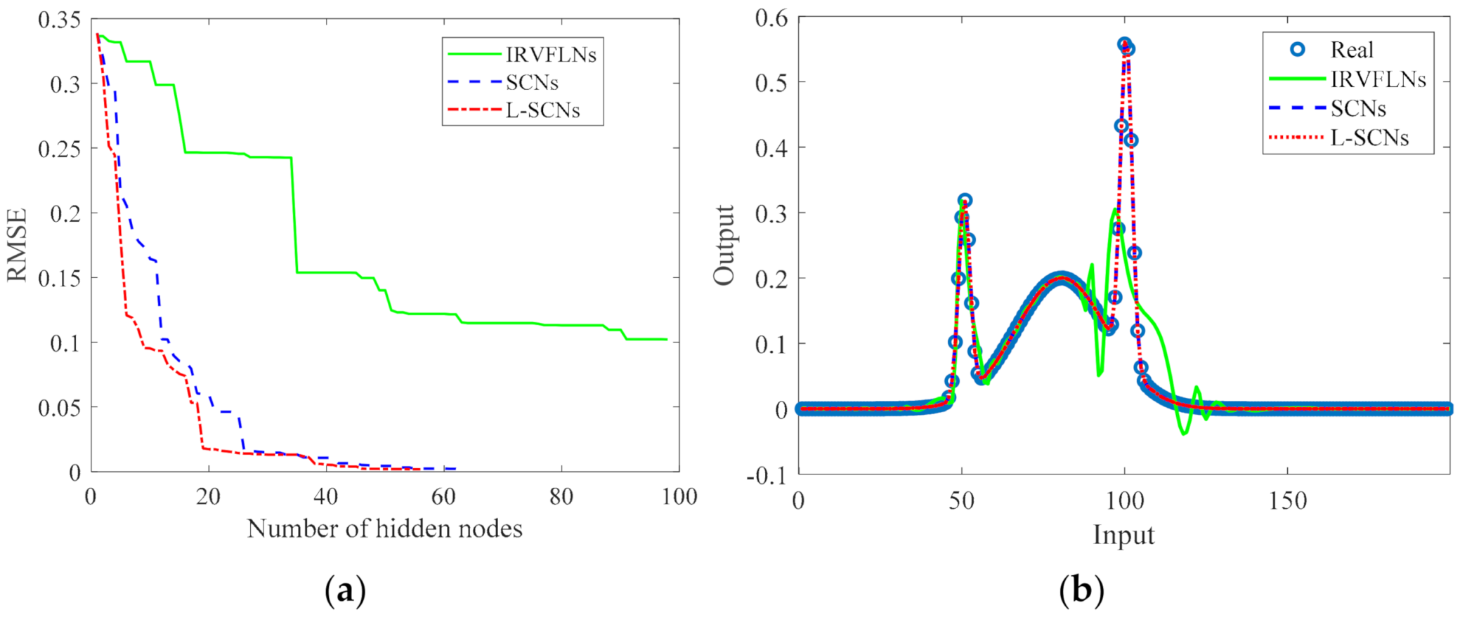
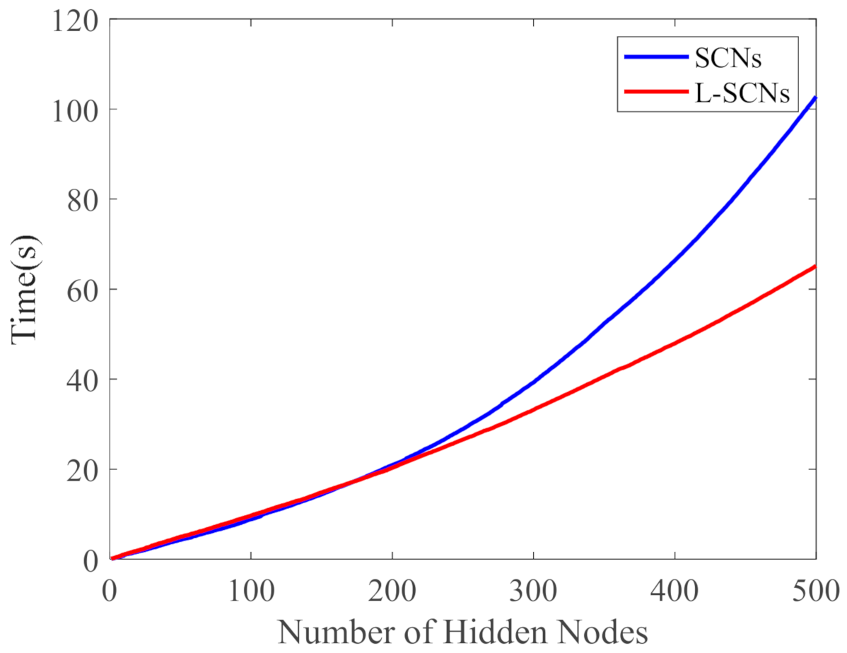
4.3. Performance Comparison

First of all, the convergence and function fitting performance of IRVFLNs, SCNs, and L-SCNs are evaluated using a highly nonlinear benchmark regression function dataset. The results shown in

Table 3. Performance comparison of highly nonlinear function.

Models	L	t (s)	Training Error	Testing Error
IRVFLNs	100	0.3657	0.0720	0.0714
SCNs	63.20	0.1500	0.0016	0.0016
L-SCNs	56.17	0.1218	0.0015	0.0014

, includes training time, training error, testing error and the number of hidden nodes, and the best experimental results are highlighted. It can be seen from Table 3 that the modeling times of L-SCNs are 18.8% and 66.69% lower than that of SCNs and IRVFLNs, respectively. The training error and testing error of L-SCNs have obvious advantages, especially compared with IRVFLNs. In addition, compared with IRVFLNs, SCNs and L-SCNs save 36.8% and 43.83% of hidden nodes, respectively. This is mainly because the hidden node parameter selection function of the supervision mechanism improves the compactness of the model while ensuring the high performance of the model. Since SCNs can only obtain approximate solutions when using M–P generalized inverse to calculate output weights, while L-SCNs output weight evaluation method can get real solutions. Therefore, L-SCNs is superior to SCNs in compactness and model performance.

In addition, in order to analyze the convergence and fitting ability of IRVFLNs, SCNs and L-SCNs, this paper draws a convergence curve and a fitting curve, as shown in Figure 2. It can be seen from the convergence curve that IRVFLNs used up 100 preset hidden nodes, but still did not meet the expected error tolerance. In particular, it is difficult to improve the convergence of IRVFLNs by adding more nodes after the number of hidden nodes reaches 51. The convergence of SCNs and L-SCNs meets the expected error tolerance, and L-SCNs converges faster. It only uses 19 nodes to reduce the residual to 0.02, and only used 56.17 nodes to meet the expectations. Compared with SCNs, L-SCNs save 11.12% of nodes. Therefore, it shows that L-SCNs modeling is faster, and the structure of the built model is more compact. The fitting curve shows that among IRVFLNs, SCNs and L-SCNs, the data fitting ability of the model built by IRVFLNs is the worst, while the models built by SCN and L-SCN have similar fitting capabilities.

IRVFLNs, SCNs and L-SCNs. The experimental results are presented

Table 4. Performance comparison for regression data sets.

Data Sets	Models	L	t (s)	Training Error	Testing Error
Abalone	IRVFLNs	100	0.2711	0.1895	0.1977
	SCNs	32.33	0.1874	0.1599	0.1641
	L-SCNs	8.67	0.1391	0.1590	0.1601
Compactiv	IRVFLNs	200	0.6385	0.1770	0.1862
	SCNs	27	0.2216	0.1465	0.1541
	L-SCNs	16.67	0.1856	0.1418	0.1501
winequality-white	IRVFLNs	100	0.5604	0.2325	0.2472
	SCNs	100	0.94	0.2276	0.2536
	L-SCNs	100	0.89	0.2264	0.2487
california	IRVFLNs	23.57	0.12	0.1088	0.1101
	SCNs	16.33	0.14	0.1178	0.1171
	L-SCNs	10.33	0.14	0.1144	0.1155
delta_ail	IRVFLNs	27.67	0.09	0.2098	0.2163
	SCNs	11.33	0.10	0.2095	0.2113
	L-SCNs	9.33	0.12	0.2029	0.2107

and

Table 5. Performance comparison for classification data sets.

Data Sets	Models	L	t (s)	Training Error	Testing Error
Iris	IRVFLNs	107.2	0.1947	0	0.1667
	SCNs	74.33	0.1424	0	0.0667
	L-SCNs	71.67	0.1237	0	0.0556
HAR	IRVFLNs	1000	59.36	0.0350	0.0763
	SCNs	264.5	26.72	0.0322	0.0747
	L-SCNs	251.5	16.02	0.0322	0.0658
wine	IRVFLNs	117.8	0.3871	0	0.1611
	SCNs	97.33	0.2615	0	0.0695
	L-SCNs	90.00	0.1722	0	0.0667

, respectively. Table 4 and Table 5 show the experimental results of the regression problem and the classification problem, respectively. For each model, the best experimental results are highlighted in Table 4 and Table 5. Table 4 gives the number of hidden nodes, the training time, the training error and the testing error. It can be seen from Table 4 that for Abalone data set, the training error and test error of IRVFLNs are the worst, and 100 hidden nodes are used up, which is also the main reason for the longest modeling time. L-SCNs and SCNs achieve similar training error and testing error, but L-SCNs saves 73.18% and 25.77% of the number of nodes and modeling time, respectively. On the Compactiv data set, IRVFLNs still used up all hidden nodes, and achieved the worst training error and testing error. The experimental results of L-SCNs and SCNs are also consistent with the results on the Abalone data set. By comparing the experimental results of winequality-white, california and delta_ail, it can be seen that: (1) When consuming the same hidden layer node, IRVFLNs modeling is the fastest, but the model performance is the worst; (2) The number of hidden nodes required for L-SCNs modeling is far less than that of the other two algorithms; (3) When the number of hidden layer nodes is small, L-SCNs has no obvious advantage in lightness. In summary, L-SCNs are superior to IRVFLN and SCNs in terms of model compactness and modeling time when a large number of hidden layer nodes are needed.

Table 5 shows the numbers of hidden node, training times, training errors and testing errors of IRVFLNs, SCNs and L-SCNs on the three real classification data sets. As can be seen from Table 5, for the Iris data set, the numbers of hidden nodes required by SCNs and L-SCNs is much less than 107.2 of IRVFLNs. Therefore, SCNS and L-SCNs have lower modeling times. The main reason behind this result is that the node parameter selection function of the supervisory mechanism makes the node parameters quality better, so the model can reach the expected value faster and perform better. Compared with SCNs, L-SCNs saves 3.58% and 5.35% in the number of hidden nodes and training time, respectively. At the same time, L-SCNs achieves the best test error. In particular, the training errors of IRVFLNs, SCNs and L-SCNs on the Iris data set is the same. For the HAR data set, compared to the other two algorithms, L-SCNs saves 74.85% and 4.91% in the number of hidden nodes, while saving 73.01% and 40.04% in training time, respectively. In addition, the number of hidden nodes of IRVFLNs reached the maximum value of 1000, but the model performance was the worst. For the wine data set, L-SCNs and SCNs still have obvious advantages in the number of hidden nodes, training time and test error. Compared with the other two algorithms, L-SCNs constructs the best performance model with the least 90 hidden nodes and the minimum 0.1722 s training time. In summary, L-SCNs have obvious merits in training efficiency and model compactness for classification tasks. Therefore, L-SCNs is a lightweight algorithm. Through the analysis of Table 1 and Table 5, it can be seen that HAR and wine data sets have higher sample numbers and features than Iris data set, especially HAR data set. The experimental results also show that L-SCNs have more obvious in lightweight on HAR and wine data sets. Therefore, L-SCNs are suitable for dealing with large data problems.

In order to further verify the advantages of L-SCNs in terms of lightweight. In this paper, while maintaining the same number of hidden nodes, the change process of modeling time of SCNs and L-SCNs with the increase of the number of hidden nodes is drawn when the experiment is performed on the HAR data set, as shown in Figure 3. It can be seen that before the hidden nodes reach 100, the modeling time of SCNs and L-SCNs is the same. However, after 100 hidden nodes, with the increase of hidden nodes, the advantage of L-SCNs becomes more and more obvious in term of lightweight. When 500 nodes are reached, the gap between SCNs and L-SCNs widened to 36.66%. It also shows that when dealing with modeling tasks that require a large number of hidden nodes, the L-SCNs proposed in this paper can effectively reduce the modeling complexity and improve the lightweight of modeling.

In addition, we have compared the Cholesky decomposition approach with other methods, including QR decomposition, LDL decomposition and SVD decomposition; the detailed results of all these approaches are shown in

Table 6. Comparison of different decomposition methods.

Methods	100	200	300	400	500
SVD	6.33 s	16.61 s	35.47 s	64.79 s	107.78 s
LDL	5.78 s	14.00 s	30.96 s	49.54 s	76.22 s
QR	5.59 s	13.69 s	26.17 s	44.03 s	69.12 s
Cholesky	5.53 s	13.48 s	25.83 s	43.67 s	68.27 s

. It can be found from Table 6 that Cholesky decomposition is slightly better than QR decomposition and LDL decomposition. However, as the number of nodes increases, compared with SVD decomposition, Cholesky decomposition has more obvious advantages in terms of lightness. The main reason for this result is that the computational complexity of QR and LDL decomposition is similar to that of Cholesky decomposition. The computational complexity of SVD far exceeds these three methods. This clearly demonstrates the lightness of Cholesky decomposition.

5. Conclusions

This work is motivated by the time-consuming calculation of output weights in each addition of hidden nodes. Lightweight stochastic configuration networks (L-SCNs) are developed by employing a non-inverse calculation method for problem solving. In L-SCNs, a positive definite equation is firstly proposed based on normal equation theory to take the place of the over-determined equation to avoid the use of M–P generalized inverse. Secondly, the Cholesky decomposition method with low computational complexity is used to calculate the positive definite equation and obtain the output weight. The proposed L-SCNs have been evaluated on several benchmark data sets, and the experimental results show that L-SCNs not only solve the high complexity problem of calculating output weights, but also improve the compactness of the model structure. In addition, the comparison with IRVFLNs and SCNs shows that L-SCNs have obvious advantages in lightweight. Therefore, L-SCNs are particularly suitable for complex modeling tasks that usually require a mass of hidden nodes to build an enormous network.

References

1. Han, F.; Jiang, I.; Ling, Q.H.; Su, B.H. A survey on metaheuristic optimization for random single-hidden layer feedforward neural network. Neurocomputing 2019, 335, 261–273. [Google Scholar] [CrossRef]
2. Tamura, S.; Tateishi, M. Capabilities of a four-layered feedforward neural network: Four layers versus three. IEEE Trans. Neural Netw. 1997, 8, 251–255. [Google Scholar] [CrossRef] [PubMed]
3. Wu, X.; Rozycki, P.; Wilamowski, B.M. A Hybrid Constructive Algorithm for Single-Layer Feedforward Networks Learning. IEEE Trans. Neural Netw. Learn. Syst. 2017, 26, 1659–1668. [Google Scholar] [CrossRef] [PubMed]
4. Igelnik, B.; Pao, Y.H. Stochastic choice of basis functions in adaptive function approximation and the functional-link net. IEEE Trans. Neural Netw. 1995, 6, 1320–1329. [Google Scholar] [CrossRef] [PubMed] [Green Version]
5. Pao, Y.H.; Takefuji, Y. Functional-link net computing: Theory, system architecture, and functionalities. Computer 1992, 25, 76–79. [Google Scholar] [CrossRef]
6. Wang, D.H.; Li, M. Stochastic Configuration Networks: Fundamentals and Algorithms. IEEE Trans. Cybern. 2017, 47, 3466–3479. [Google Scholar] [CrossRef] [Green Version]
7. Wang, D.H.; Cui, C.H. Stochastic Configuration Networks Ensemble for Large-Scale Data Analytics. Inf. Sci. 2017, 417, 55–71. [Google Scholar] [CrossRef] [Green Version]
8. Dai, W.; Li, D.P.; Zhou, P.; Chai, T.Y. Stochastic configuration networks with block increments for data modeling in process industries. Inf. Sci. 2019, 484, 367–386. [Google Scholar] [CrossRef]
9. Tian, Q.; Yuan, S.J.; Qu, H.Q. Intrusion signal classification using stochastic configuration network with variable increments of hidden nodes. Opt. Eng. 2019, 58, 026105.1–026105.8. [Google Scholar] [CrossRef]
10. Dai, W.; Zhou, X.Y.; Li, D.P.; Zhu, S.; Wang, X.S. Hybrid Parallel Stochastic Configuration Networks for Industrial Data Analytics; IEEE Transactions on Industrial Informatics: Piscataway, NJ, USA, 2021. [Google Scholar] [CrossRef]
11. Wang, D.H.; Li, M. Robust Stochastic Configuration Networks with Kernel Density Estimation for Uncertain Data Regression. Inf. Sci. 2017, 412, 210–222. [Google Scholar] [CrossRef]
12. Li, M.; Huang, C.Q.; Wang, D.H. Robust stochastic configuration networks with maximum correntropy criterion for uncertain data regression. Inf. Sci. 2018, 473, 73–86. [Google Scholar] [CrossRef]
13. Wang, D.H.; Li, M. Deep Stochastic Configuration Networks: Universal Approximation and Learning Representation. In Proceedings of the IEEE International Joint Conference on Neural Networks, Anchorage, AK, USA, 14–19 May 2017. [Google Scholar]
14. Pratama, M.; Wang, D.H. Deep Stacked Stochastic Configuration Networks for Non-Stationary Data Streams. Inf. Sci. 2018, 495, 150–174. [Google Scholar] [CrossRef] [Green Version]
15. Lu, J.; Ding, J.L. Construction of prediction intervals for carbon residual of crude oil based on deep stochastic configuration networks. Inf. Sci. 2019, 486, 119–132. [Google Scholar] [CrossRef]
16. Li, M.; Wang, D.H. 2-D Stochastic Configuration Networks for Image Data Analytics. IEEE Trans. Cybern. 2021, 51, 359–372. [Google Scholar] [CrossRef]
17. Lu, J.; Ding, J.L.; Dai, X.W.; Chai, T.Y. Ensemble Stochastic Configuration Networks for Estimating Prediction Intervals: A Simultaneous Robust Training Algorithm and Its Application. IEEE Trans. Neural Netw. Learn. Syst. 2020, 31, 5426–5440. [Google Scholar] [CrossRef] [PubMed]
18. Lu, J.; Ding, J.L.; Liu, C.X.; Chai, T.Y. Hierarchical-Bayesianbased sparse stochastic configuration networks for construction of prediction intervals. IEEE Trans. Neural Netw. Learn. Syst. 2021, 1–2. [Google Scholar] [CrossRef]
19. Lu, J.; Ding, J.L. Mixed-distribution-based robust stochastic configuration networks for prediction interval construction. IEEE Trans. Ind. Inform. 2020, 16, 5099–5109. [Google Scholar] [CrossRef]
20. Sheng, Z.Y.; Zeng, Z.Q.; Qu, H.Q.; Zhang, Y. Optical fiber intrusion signal recognition method based on TSVD-SCN. Opt. Fiber Technol. 2019, 48, 270–277. [Google Scholar] [CrossRef]
21. Xie, J.; Zhou, P. Robust Stochastic Configuration Network Multi-Output Modeling of Molten Iron Quality in Blast Furnace Ironmaking. Neurocomputing 2020, 387, 139–149. [Google Scholar] [CrossRef]
22. Zhao, J.H.; Hu, T.Y.; Zheng, R.F.; Ba, P.H. Defect Recognition in Concrete Ultrasonic Detection Based on Wavelet Packet Transform and Stochastic Configuration Networks. IEEE Access 2021, 99, 9284–9295. [Google Scholar] [CrossRef]
23. Salmerón, M.; Ortega, J.; Puntonet, C.G.; Prieto, A. Improved RAN sequential prediction using orthogonal techniques. Neurocomputing 2001, 41, 153–172. [Google Scholar] [CrossRef]
24. Qu, H.Q.; Feng, T.L.; Zhang, Y. Ensemble Learning with Stochastic Configuration Network for Noisy Optical Fiber Vibration Signal Recognition. Sensors 2019, 19, 3293. [Google Scholar] [CrossRef] [Green Version]
25. Liu, J.; Hao, R.; Zhang, T.; Wang, X.Z. Vibration fault diagnosis based on stochastic configuration neural networks. Neurocomputing 2021, 434, 98–125. [Google Scholar] [CrossRef]
26. Krein, S.G. Overdetermined Equations; Birkhäuser: Basel, Switzerland, 1982. [Google Scholar]
27. Loboda, A.V. Determination of a Homogeneous Strictly Pseudoconvex Surface from the Coefficients of Its Normal Equation. Math. Notes 2003, 73, 419–423. [Google Scholar] [CrossRef]
28. Roverato, A. Cholesky decomposition of a hyper inverse Wishart matrix. Biometrika 2000, 87, 99–112. [Google Scholar] [CrossRef]
29. Anguita, S.; Ghio, A.; Oneto, L.; Parra, X. Energy efficient smartphone-based activity recognition using fixed-point arithmetic. J. Univers. Comput. 2013, 19, 1295–1314. [Google Scholar]
30. Fdez, J.A.; Fernandez, A.; Luengo, J.; Derrac, J.; Garacia, S.; Herrera, F. KEEL Data-Mining Software Tool: Data Set Repository, Integration of Algorithms and Experimental Analysis Framework. J. Mult.-Valued Log. Soft Comput. 2011, 17, 255–287. [Google Scholar]
31. Tyukin, I.Y.; Prokhorov, D.V. Feasibility of random basis function approximators for modeling and control. In Proceedings of the IEEE Control Applications, (CCA) & Intelligent Control, St. Petersburg, Russia, 8–10 July 2009; pp. 1391–1396. [Google Scholar]
32. Li, M.; Wang, D.H. Insights into randomized algorithms for neural networks: Practical issues and common pitfalls. Inf. Sci. 2017, 382, 170–178. [Google Scholar] [CrossRef]
Figure 1. Network structure of SCNs. 1, 2, j, j + 1 represent the node 1, 2, j, j + 1 respectively. d represents the dimension of the input data set and m represents the dimension of the output data.
Electronics 11 00262 g001
Figure 2. Training results of three algorithms. (a) Convergence Curve; (b) Fitting Curve.
Electronics 11 00262 g002
Figure 3. Modeling time of SCNs and L-SCNs.
Electronics 11 00262 g003