Reducing Parameters of Neural Networks via Recursive Tensor Approximation

Abstract

Large-scale neural networks have attracted much attention for surprising results in various cognitive tasks such as object detection and image classification. However, the large number of weight parameters in the complex networks can be problematic when the models are deployed to embedded systems. In addition, the problems are exacerbated in emerging neuromorphic computers, where each weight parameter is stored within a synapse, the primary computational resource of the bio-inspired computers. We describe an effective way of reducing the parameters by a recursive tensor factorization method. Applying the singular value decomposition in a recursive manner decomposes a tensor that represents the weight parameters. Then, the tensor is approximated by algorithms minimizing the approximation error and the number of parameters. This process factorizes a given network, yielding a deeper, less dense, and weight-shared network with good initial weights, which can be fine-tuned by gradient descent.

1. Introduction

Large neural networks such as convolutional neural networks have demonstrated state-of-the-art performance in a number of benchmarks in computer vision, automatic speech recognition, natural language processing, audio recognition, etc. [1,2,3,4]. However, these networks have millions and billions of parameters [5], and the evaluation of such models is computationally demanding. While the enormous computing power available today, mainly driven by GPUs, makes us consider the evaluation easy, it comes with large energy consumption. In embedded platforms, the evaluation is still challenging because resources such as computing power, memory, storage, and energy are highly limited. The large energy consumption can also be a critical issue in data centers and can restrict the computing capacity.

Fortunately, weight parameters in neural networks are heavily redundant [6], and exploiting the redundancy, computational cost, and space requirements can be minimized while maintaining the performance. To this end, several methods have been proposed very recently [7,8,9,10,11,12], and all of these methods assume that neural networks are executed in stored-program computers, including GPU-based machines. The traditional computers have several processing bottlenecks, such as limited memory-bandwidth and a limited number of processing elements, and the performance benefit (e.g., speed-up) by the parameter reduction is not as high as the reduction rate.

Emerging neuromorphic computers emulate biological neural networks, and silicon synapses and neurons are processing elements [13,14]. Connections and units in neural networks are mapped to synapses and neurons, respectively, and these computational resources are not time-multiplexed as in the traditional computers. Thus, the runtime is not a concern because it does not depend on the size of the models. The size of the models affects the required synapses and neurons. To store weight parameters within synapses or nearby, neuromorphic computers use low-density on-chip memories and equip with at least as many synapses as the parameters [13,15,16,17]. Without weight-sharing, the number of synapses equals the number of weight parameters. Thus, the number of parameters itself is a very important metric in neuromorphic computers because each weight parameter requires a synpase, a computational resource with its own dedicated memory in neuromorphic systems [18]. In [19], the authors reduced the number of parameters for neuromorphic systems by combining matrix factorization and pruning. Thus, it can be applied to fully connected layers only and cannot take advantage of redundancy across multiple dimensions in high-order tensors.

In this paper, we describe a general parameter reduction method using new tensor approximation methods based on divide-and-conquer [20]. This technique can be applied to store-program computers as well as neuromorphic computers. However, unlike previous works, our main objective was to reduce the size of the models for neuromorphic computers, so we consider the number of parameters as the figure of merit.

This paper makes the following contributions: (1) For neuromorphic computers, we evaluated the methods for reducing the size of the models in terms of the parameter reduction. (2) We approximated a tensor using a more expressive format than the canonical polyadic (CP) format [9], which has been commonly used recently and has shown that higher expressiveness can lead to a better quality of results. (3) For a convolutional network, we compressed all the layers, including fully-connected layers, using a single method and demonstrated that the network with all layers compressed could perform similarly to the original network. (4) We show that the weights of the first fully-connected layers can be tensor-approximated effectively.

2. Related Work

Denil et al. [6] showed that weight parameters are highly redundant by representing a weight matrix as a product of two low-rank matrices. This implies that neural networks are heavily over-parameterized. Their work ignited recent interest in exploiting the massive redundancy to minimize cost at test time.

A group of works [7,8,9] used the redundancy to speed up the evaluation of convolutional neural networks. They reduced the number of parameters from a trained network by finding low-rank approximations to weight tensors. Jaderberg et al. [7] approximated the 4-tensor representing a convolutional kernel as a composition of two 3-tensors and obtained parameters that minimized the difference between the outputs of the original and approximated layers using training data. Denton et al. [8] combined filter clustering and a 3-tensor approximation method to approximate a 4-tensor. For the first convolutional layer and the higher convolutional layers, different clustering methods were employed, and for the fully connected layers, low-rank matrix approximation was used. They also suggested fine-tuning the layers above the approximated one when the accuracy is degraded after approximation. Between the two 3-tensor approximation methods they used, the one that produced better results approximated a 3-tensor to a sum of separable 3-tensors, which is known as canonical polyadic (CP) decomposition [9]. They demonstrated 2× speed-ups of convolutional layers within a 1% accuracy drop. Lebedev et al. [9] used CP decomposition for 4-tensors and fine-tuned the whole network. They demonstrated better speed-up (e.g., 4× speed-up of a convolutional layer) than the previous methods. In the meantime, they also reported a failure in a fine-tuning that they suspected was caused by the instability of CP decomposition. In the CP format, the tensor approximation problem with a given rank is known to be unstable, and robust numerical procedures such as singular value decomposition (SVD) [21] are in effect not available [22].

To achieve the same goal of fast feedforward execution, Jin et al. [10] trained a network with a small number of parameters in the first place. They applied structural constraints to obtain two separable 3-tensors for each output channel in convolutional layers and achieved 2× speed-up for the forward pass of the whole network. While reducing the number of parameters decreases the storage and memory requirement, parameters in convolutional layers take up a small portion of the total parameters. In order to reduce the memory footprint specifically, Yang et al. [11] replaced all fully connected layers with a kernel machine. The space overhead could be minimized by finding a compact representation for weights as well as by reducing the number of parameters. Gong et al. [12] performed scalar quantization using k-means clustering for weights in fully connected layers. This type of method can be combined with parameter reduction methods.

Our work differs from previous works in several ways. First, we aimed to minimize the cost in executing neural networks on neuromorphic computers. To this end, we chose the number of parameters as our cost metric. Second, we propose a new tensor approximation algorithm based on divide-and-conquer [20] and achieved up to 154× reduction in weight parameters within a 1% accuracy drop. To the best of our knowledge, such a high reduction rate has not been reported yet. Last, our method does not have certain limitations that some of the recent methods have. Our method is numerically stable and can be applied to both convolutional layers and fully connected layers. Moreover, the resulting reduced network is end-to-end trainable.

3. Tensor Factorization

In a convolutional neural network for computer vision tasks, the weights in a convolutional layer or the first fully connected layer can be represented in a 4th-order tensor, and we propose a tensor factorization (approximation) method for a weight tensor.

3.1. Existing Methods

For high-order tensor decomposition, several methods are known, such as CP decomposition and Tucker decomposition (also known as high-order singular value decomposition) [23]. In the CP format, the tensor approximation problem with a given rank is known to be unstable, and robust numerical procedures such as the SVD are in effect not available [22]. Tucker decomposition can be computed via several SVDs, but the number of parameters after the decomposition still depends on the dimension exponentially. To tackle this issue, new methods such as tensor-train decomposition [24] and hierarchical Tucker decomposition [25] have been proposed. These methods are different from the proposed method, and they involve complex operations that are difficult to implement in neuromorphic systems, with exception of CP decomposition. We compare our method with CP decomposition later in this paper.

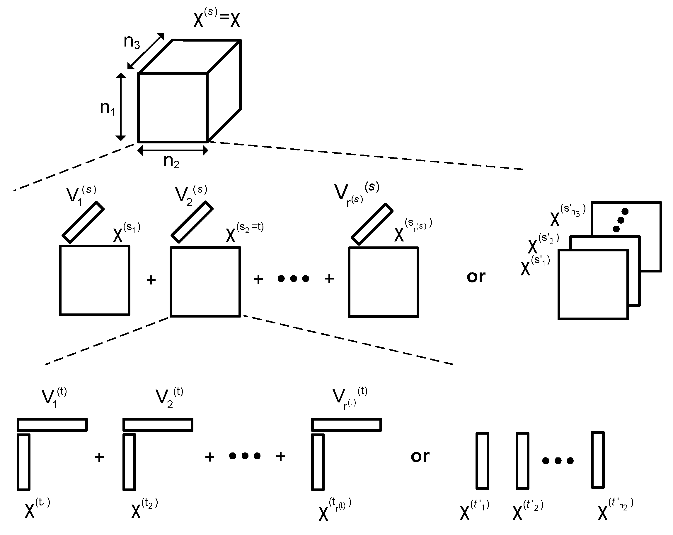
3.2. Proposed Factorization Method

Definition 1.

The d-mode matricization of a tensor $\chi \in {\mathbb{R}}^{n_1\times n_2\times \cdots \times n_d}$ is a matrix defined by $\mathcal{M}:{\mathbb{R}}^{n_1\times n_2\times \cdots \times n_d}\to {\mathbb{R}}^{n_d\times n_1{n}_2\cdots n_{d-1}}$, ${\left(\mathcal{M}\left(\chi \right)\right)}_{i_d,(i_1,...,i_{d-1})}={\chi }_{i_1,i_2,\cdots ,i_d}$ for any indices $(i_1,\cdots ,i_d)$ in the multi-index set $\{1,\cdots ,n_1\}\times \cdots \times \{1,\cdots ,n_d\}$.

Definition 2.

The vectorization of a tensor $\chi \in {\mathbb{R}}^{n_1\times n_2\times \cdots \times n_d}$ is a vector defined by $\mathcal{V}:{\mathbb{R}}^{n_1\times n_2\times \cdots \times n_d}$$\to {\mathbb{R}}^{n_1{n}_2\cdots n_d}$, ${\left(\mathcal{V}\left(\chi \right)\right)}_{(i_1,...,i_d)}={\chi }_{i_1,i_2,\cdots ,i_d}$ for any indices $(i_1,\cdots ,i_d)$ in the multi-index set $\{1,\cdots ,n_1\}\times \cdots \times \{1,\cdots ,n_d\}$.

We assume the reverse lexicographical order of the multi-indices throughout this paper. We now propose a tensor factorization method based on divide-and-conquer [20].

Definition 3.

A decomposition tree $\mathcal{T}$ of a tensor χ is a tree such that (1) each node s is associated with a tensor ${\chi }^{\left(s\right)}$, (2) each node has two types of successors, (3) the tensor corresponding to a node is composed of the tensors of its successors of one type, and (4) the root is associated with χ. The successor sets are denoted by $S^a$ and $S^b$, respectively.

Given a tensor $\chi \in {\mathbb{R}}^{n_1\times n_2\times \cdots \times n_e}$, we recursively construct $\mathcal{T}\left(\chi \right)$ from the root node. For a node s, the successors of the first type are constructed by the SVD. Let ${\chi }^{\left(s\right)}$ be a d-th order tensor of shape $n_1\times n_2\times \cdots \times n_d$. The SVD for the transpose of $\mathcal{M}\left(\chi \right)$ yields

$$\mathcal{M}{\left({\chi }^{\left(s\right)}\right)}^T={\mathbf{U}}^{\left(s\right)}{\Sigma }^{\left(s\right)}{{\mathbf{V}}^{\left(s\right)}}^T.$$

(1)

Let $S^a\left(s\right)=\{s_1,\cdots ,s_{r^{\left(s\right)}}\}$, where $r^{\left(s\right)}$ is the rank of $\mathcal{M}\left({\chi }^{\left(s\right)}\right)$. Each left-singular vector (i.e., the column vectors of ${\mathbf{U}}^{\left(s\right)}$) is reshaped into a tensor of shape $n_1\times n_2\times \cdots \times n_{d-1}$ such that the left-singular vector is the vectorization of the tensor, which results in $r^{\left(s\right)}$ (d-1)th order tensors. These are ${\chi }^{\left(s_1\right)},...,{\chi }^{\left(s_r\right)}$. Thus, we can write

$${\mathbf{U}}^{\left(s\right)}=[\mathcal{V}\left({\chi }^{\left(s_1\right)}\right)\cdots \mathcal{V}\left({\chi }^{\left(s_r\right)}\right)].$$

(2)

For the node s, the successors of the second type are constructed by subtensors. Let $S^b\left(s\right)=\{s_1^{\prime },\cdots ,s_{n_d}^{\prime }\}$. We obtain the subtensors by fixing the highest order index (i.e., the d-mode), and they become ${\chi }^{\left(s_1^{\prime }\right)},...,{\chi }^{\left(s_{n_d}^{\prime }\right)}$. Thus, we produce $r^{\left(s\right)}+n_d$ one-level lower-order tensors in total using both the methods. Given a tensor, we apply this procedure recursively until it produces vectors (i.e., 1st-order tensors). Since we break the same tensors in the two ways during the recursion, we have two possible factored forms for each tensor and choose either one of them. This allows us to explore numerous factored forms and make our model very expressive.

Let us denote the number of parameters of the tensor associated with a node s by ${\eta }^{\left(s\right)}$. Since ${\Sigma }^{\left(s\right)}$ can be collapsed into either ${\mathbf{U}}^{\left(s\right)}$ or ${\mathbf{V}}^{\left(s\right)}$, the number of parameters ${\eta }^{\left(s\right)}$ in ${\chi }^{\left(s\right)}$ after the factorization becomes ${\Sigma }_i^{r^{\left(s\right)}}{\eta }^{\left(s_i\right)}+r^{\left(s\right)}{n}_d$ if the SVD form is taken. If the subtensor form is taken, ${\eta }^{\left(s\right)}={\Sigma }_i^{n_d}{\eta }^{\left(s_i^{\prime }\right)}$.

Let $x_{i_1,\cdots ,i_d}^{\left(s\right)}={\chi }_{i_1,\cdots ,i_d}^{\left(s\right)}$, $v_{i_d,j}^{\left(s\right)}={\mathbf{V}}_{i_d,j}^{\left(s\right)}$, and ${\lambda }_j^{\left(s\right)}={\Sigma }_{j,j}^{\left(s\right)}$. Our tensor decomposition can also be written in an elementwise form as

$$x_{i_1,i_2,\cdots ,i_d}^{\left(s\right)}={\alpha }^{\left(s\right)}\sum _j^{r^{\left(s\right)}}{\lambda }_j^{\left(s\right)}{x}_{i_1,\cdots ,i_{d-1}}^{\left(s_j\right)}{v}_{i_d,j}^{\left(s\right)}+(1-{\alpha }^{\left(s\right)})x_{i_1,\cdots ,i_{d-1}}^{\left(s_{i_d}^{\prime }\right)},$$

(3)

where ${\alpha }^{\left(s\right)}$ is a binary free variable that can be set to either one or zero. The decomposition for a 3rd-order tensor is depicted in Figure 1.

3.3. Low-Rank Tensor Approximation

The parameter reduction by the factorization is usually possible when $r^{\left(s\right)}$ is small. Thus, we perform low-rank approximation with the factorization. Since we break a tensor down into smaller, lower-order tensors, the problem of approximating a tensor is now solved by combing small, approximated tensors into a larger tensor. If a tensor is broken down by the SVD, the approximation ${\tilde{\chi }}^{\left(s\right)}$ to the original tensor is obtained as follows: (i) small singular values are replaced by zero, and (ii) ${\chi }^{\left(s_i\right)}$ is approximated by ${\tilde{\chi }}^{\left(s_i\right)}$. If a tensor is broken down into the $n_d$ subtensors, its approximation is simply obtained by combing the approximations to the $n_d$ subtensors. Since a tensor is broken down in both ways, we can choose one of the two approximations to the tensor.

To approximate the given tensor $\chi$ using the decomposition, we zero-out small singular values in a recursive manner. For this, we introduce another binary variable ${\beta }^{\left(s\right)}$ and write the approximated tensor ${\tilde{\chi }}^{\left(s\right)}$ in an elementwise form as

$${\tilde{x}}_{i_1,i_2,\cdots ,i_d}^{\left(s\right)}={\alpha }^{\left(s\right)}\sum _j^{r^{\left(s\right)}}{\lambda }_j^{\left(s\right)}{\beta }_j^{\left(s\right)}{\tilde{x}}_{i_1,\cdots ,i_{d-1}}^{\left(s_j\right)}{v}_{i_d,j}^{\left(s\right)}+(1-{\alpha }^{\left(s\right)}){\tilde{x}}_{i_1,\cdots ,i_{d-1}}^{\left(s_{i_d}^{\prime }\right)},$$

(4)

Unlike the standard low-rank approximation method, we can zero-out a singular value when a smaller singular value than that remains. That is, we do not necessarily zero-out trailing singular values. Thus, we use the set of the binary values ${\beta }_1^{\left(s\right)},\cdots ,{\beta }_{r^{\left(s\right)}}^{\left(s\right)}$ instead of the target rank. We define the approximation error by

$${ϵ}^{\left(s\right)}\triangleq {\parallel {\chi }^{\left(s\right)}-{\tilde{\chi }}^{\left(s\right)}\parallel }_F^2.$$

(5)

where ${\parallel \parallel }_F$ is the Frobenius norm. Then, the approximation error by the proposed method is

$${ϵ}^{\left(s\right)}={\alpha }^{\left(s\right)}\sum _{j=1}^{r^{\left(s\right)}}{{\lambda }_j^{\left(s\right)}}^2\left({\beta }_j^{\left(s\right)}+(1-{\beta }_j^{\left(s\right)}){ϵ}^{\left(s_j\right)}\right)+(1-{\alpha }^{\left(s\right)})\sum _{j=1}^{n_d}{ϵ}^{\left(s_j^{\prime }\right)}$$

(6)

since ${\mathbf{U}}^{\left(s\right)}$ and ${\mathbf{V}}^{\left(s\right)}$ are orthogonal matrices.

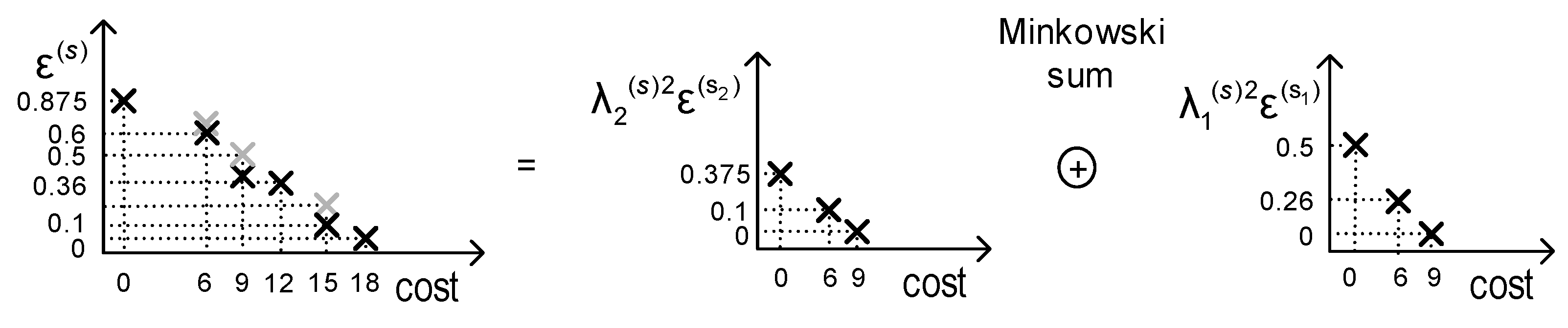
4. Dual-Objective Optimization

The choices between the two possible approximations and the decisions on the zero-out through the recursion lead to various candidate solutions to the problem of approximating a tensor. Our objective is to minimize both the approximation error and the number of parameters. For this dual-objective optimization, we use two algorithms. The first algorithm finds Pareto optimal solutions in a recursive manner with several pruning methods. The second algorithm is a greedy algorithm that takes a threshold value as input and determines singular values to zero out using the value. This algorithm chooses the one with a smaller cost between the two possible approximations.

4.1. Pareto Front Method

To tackle the optimization problem, we compute the Pareto front in a recursive manner. A tuple (l,m) corresponds to a possible approximation to a tensor, where l and m are the cost and the approximation error, respectively, representing the results of the approximation. We call the tuple the option. As an inductive hypothesis, we suppose that for each ${\chi }^{\left(s_1\right)},\cdots ,{\chi }^{\left(s_{r^{\left(s\right)}}\right)}$ generated by ${\chi }^{\left(s\right)}$, we have a Pareto optimal set of options in Figure 2. Since the approximation to ${\chi }^{\left(s\right)}$ is a composition of the approximations to the one-level lower-order tensors, an option for ${\chi }^{\left(s\right)}$ is associated with a combination of options, each from each Pareto optimal set. In order to obtain the set of options for ${\chi }^{\left(s\right)}$ from all the Pareto sets, the approximation errors in the Pareto set for ${\chi }^{\left(s_j\right)}$ are multiplied by ${\lambda }_j^{\left(s\right)}$ for $j=1,\cdots ,r^{\left(s\right)}$. Then, the set of options for ${\chi }^{\left(s\right)}$ is the Minkowiski sum of all the Pareto optimal sets. We also suppose that for each d-mode subtensor of ${\chi }^{\left(s\right)}$, we have a Pareto optimal set of options. We also perform the Minkowiski operation. Then, we have two option sets for ${\chi }^{\left(s\right)}$. Since we can choose either one of the approximations, we perform the union operation for the two sets and non-Pareto optimal options are discarded, resulting in the Pareto optimal set for ${\chi }^{\left(s\right)}$. In this manner, we obtain the final Pareto optimal set for $\chi$. When ${\chi }^{\left(s\right)}$ is a matrix, we just perform the $k^{\left(s\right)}$-rank approximation for $k^{\left(s\right)}=1,...,\lfloor n_1{n}_2/(n_1+n_2)\rfloor$, which yields a Pareto optimal set. A larger rank than these values results in a larger cost than the non-approximated one.

4.2. Greedy Method

We also use a greedy algorithm for the optimization problem. This algorithm takes a threshold value $\tau$ as input and zero-outs trailing singular values as the standard low-rank approximation method, and the target rank is denoted by $k^{\left(s\right)}$. We determine $k^{\left(s\right)}$ based on the approximation error to $\chi$ per unit cost. Thus, we set $k^{\left(s\right)}$ to the largest integer $j\le r^{\left(s\right)}$ such that

$$\frac{{\psi }^{\left(s_j\right)}}{n_1\times n_2\times \cdots \times n_{d-1}+n_d}>\tau$$

(7)

where ${\psi }^{\left(s_j\right)}={{\lambda }_j^{\left(s\right)}}^2{\psi }^{\left(s\right)}$, ${\psi }^{\left(s_j^{\prime }\right)}={\psi }^{\left(s\right)}$, and ${\psi }^{\left(\varphi \right)}=1$. To determine ${\alpha }^{\left(s\right)}$, we compare the costs of the two possible approximations and take the one with a smaller cost.

5. Application to Weight Tensors

Let $\chi \in {\mathbb{R}}^{K_h\times K_w\times C\times F}$ be the weight tensor of a convolutional layer (a fully connected layer), where $K_h$ and $K_w$ are the height and width of the kernel (the input map), respectively, C is the number of input channels, and F is the number of output feature maps. We assume that this tensor is approximated by the greedy method without loss of generality, and we further assume that ${\alpha }^{\left(s\right)}=1$ for all nodes s in $\mathcal{T}\left(\chi \right)$. Let $L_i$ be the set of the nodes at level i in $\mathcal{T}\left(\chi \right)$. Then we define

$$R_i=\sum _{s\in L_i}{k}^{\left(s\right)}$$

(8)

for $i=1,\cdots ,3$. In the greedy method, we can enforce $k^{\left(s\right)}$ to 1 for every node $s\in L_2\cup L_3$. Then, our method comes to use the CP-format, and we have $R_1=R_2=R_3$. Our decomposition method factorizes the original layer into five sublayers. If we represent the weights of each sublayer in the same format as those of the original layer, the weight tensors of the sublayers are of shape $1\times 1\times C\times R_2$, $K_h\times 1\times R_2\times R_3$, $1\times K_w\times R_3\times R_3$, $1\times 1\times R_3\times R_1$, and $1\times 1\times R_1\times F$, respectively. If the original layer is convolutional, the sublayers are also convolutional. Note that these layers are sparsely connected across channels.

Fine-Tuning

Artificial neural networks are known to be error tolerant. As we reduce the number of parameters, the approximation error increases, but the performance of the networks can remain the same due to the resilience. However, despite the resilience, the performance of ANNs will drop in the end, as the network diverges from the original one. In the dual-objective optimization, the approximate error is a surrogate metric to evaluate the quality of networks. The true metric is the performance of ANNs, such as classification accuracy. To maximize the performance of ANNs while minimizing the number of parameters, the reduced parameters can be fine-tuned against the training data.

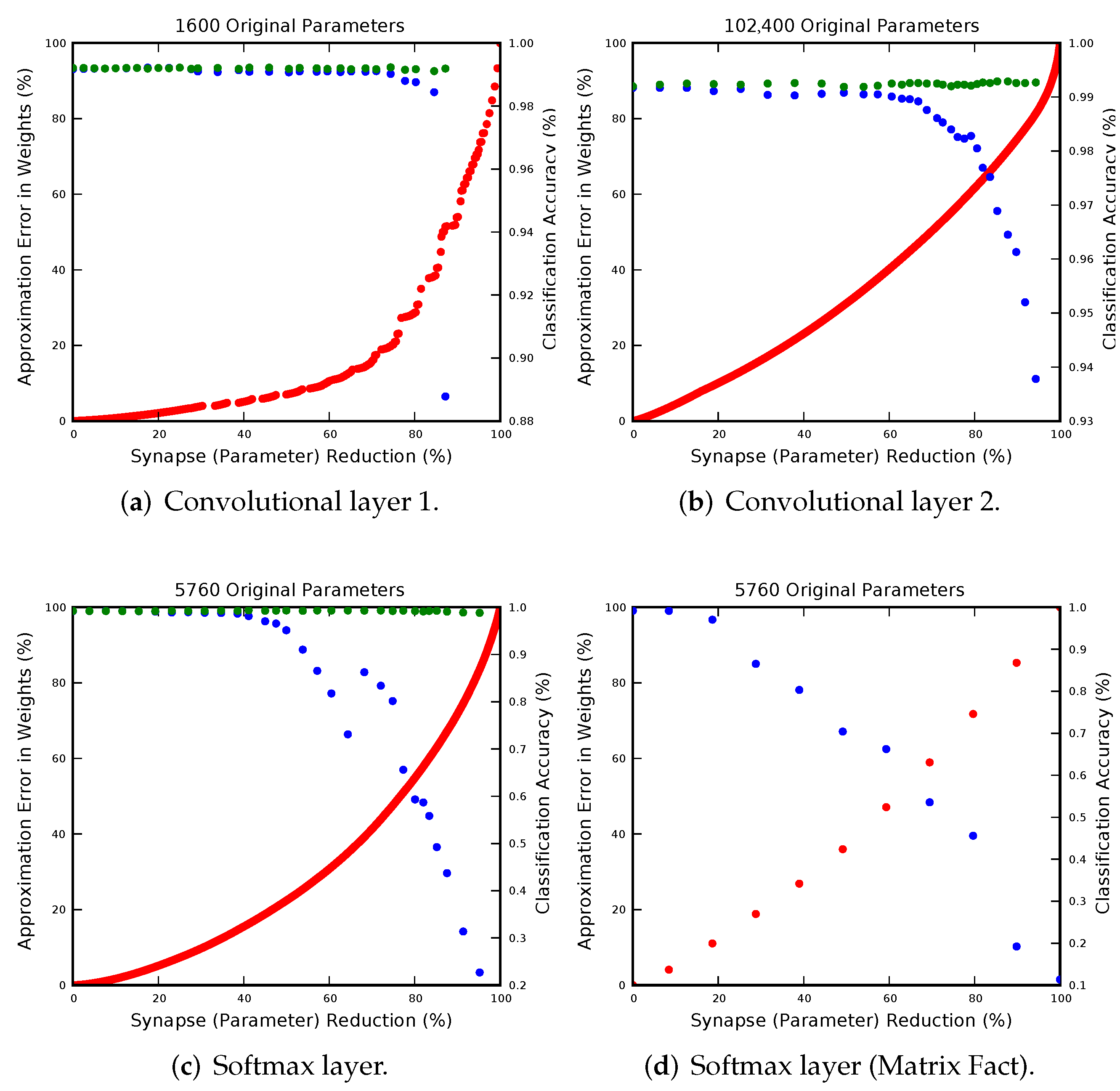
6. Experiments

We implemented the proposed algorithms in Python on top of Pylearn2 [26]. The proposed methods were evaluated on MNIST, CIFAR-10, and ILSVRC 2012 image classification datasets. We used a convolutional neural network (CNN) for MNIST. The network had two convolutional layers with 5 × 5 filters and a final softmax layer. Each convolutional layer included a max-pooling with sizes of 4 and strides of 2 and the rectified linear unit as the activation function. The weight decay was set to 0.00005; the momentum was set to 0.5; the learning rate was set to 0.01. The baseline model had 109,760 parameters and achieved 99.18% classification accuracy after training for 33 epochs. Our method can be applied to any layer, and we first performed layer-wise experiments. The results are shown in Figure 3. The classification accuracy dropped gradually as the approximation error increased, which shows that the surrogate metric to evaluate the quality of networks worked well. The second convolutional layer had 102,400 parameters, which was 93.3% of the total parameters. When we reduced it by 43× to 2375 parameters, the classification accuracy dropped to 76.45%. However, after fine-tuning the factored network again for 30 epochs, including the other layers, the accuracy was recovered to 99.25%. Thus, we achieved the 43× reduction without loss of accuracy. If some accuracy loss would have been acceptable, we could have reduced it by 164× to 627 parameters at the cost of 0.75% accuracy loss.

For the following experiments, we used the greedy algorithm. We used a CNN described in [27] for CIFAR-10. The network had three convolutional maxout layers, a fully connected maxout layer, and a fully connected softmax layer. The baseline model achieved 88.29% accuracy. We performed experiments on the fully connected maxout layer with 12 M parameters, which was 73.9% of the total parameters. We reduced it by 154× to 77.8 K at the expense of 0.9% accuracy drop.

We used AlexNet [1] implemented in [28] for ILSVRC 2012. The network contained five convolutional layers and three fully connected layers. The baseline model achieved 56.4% top-1 accuracy. We performed experiments on the first fully connected layer with 37.7 M parameters, which was 61.9% of the total parameters. We reduced it by 28× to 1.3 M parameters at the expense of 0.83% top-1 accuracy drop. We could have reduced it further by 58× to 654 K parameters by sacrificing 2.25% top-1 accuracy.

Comparison with Existing Parameter Reduction Techniques

Since all the existing methods use different neural network architectures, learning techniques, hyperparameters, and data sets, it is difficult to compare them directly. Nevertheless, we mention some results here that can be roughly compared with our results. Considering that we did not use any adaption and dropout to keep the MNIST experiments simple, our MNIST results may be compared with the jointly trained Fastfood-1024 in [11], which had 38,821 total parameters and achieved 0.83% error. When we applied our techniques to the layer with the largest number of parameters only, the resulting network had 9375 total parameters and achieved 0.75% error. When we applied our technique to all the layers, the resulting network had 3270 total parameters and achieved 0.81% error. The results are summarized in

Table 1. Parameter reduction results on MNIST dataset.

Methods	Layer	Baseline		Reduced Model
		Params	Error	Params	Error
[11]	Conv. layers	25,500	0.87%	25,500	0.83%
	FC layer	405,000		13,321
[10]	Conv. layer 1	7200	0.38%	7200	0.44%
	Conv. layer 2	307,200		30,912
	Conv. layer 3	819,200		102,144
	FC layers	NA		NA
CP-decomp.	Conv. layer 1	1600	0.82%	600	1.14%
	Conv. layer 2	102,400		828
	FC layer	5760		1920
This work	Conv. layer 1	1600	0.82%	588	0.81%
	Conv. layer 2	102,400		824
	FC layer	5760		1858

. The resulting model by our method was very small compared with the other models.

For a recent method based on CP decomposition [9], we performed a direct comparison by implementing it within our environments. We used alternating least squares (ALS) for CP decomposition. The method usually finds a better approximation to a given tensor with a same cost budget. This seems to be caused by the facts that (1) we find orthogonal vectors during the SVD, and (2) our method approximates decomposed tensors independently. Better approximation provides a good initial solution to the fine-tuning after approximation, and the initial solution can be close to the original solution. However, a slightly worse starting point is easily compensated for during the fine-tuning. Our factored form was a generalization to the CP format and was more expressive. This expressiveness paid off after the fine-tuning. We set the target rank of CP decomposition such that the number of parameters would become similar to that of our reduced model. In CP decomposition, the sizes of resulting models are coarse-grained, and the reduced model by CP decomposition was slightly larger than our reduced model. We fine-tuned the approximated model using learning rates 0.01, 0.001, and 0.0001, and the best result was selected, which is also shown in Table 1. In the previous experiment for CIFAR-10, the greedy algorithm achieved 87.42% accuracy when the size of the first fully connected layer was reduced to 77,750 parameters. For the same experiment, the CP decomposition achieved 86.31% accuracy when it was reduced to 78,358 parameters.

7. Discussion

As a part of our research toward building a neuromorphic computer that forward-executes neural networks with minimum energy consumption, we presented a parameter reduction technique based on our own tensor approximation method and achieved up to 154× reduction within negligible loss of performance.

The proposed method provided an enormous reduction rate for convolutional layers and first densely connected layers. For subsequent densely connected layers, the proposed method was reduced to the standard low-rank approximation method. A possible research direction for future works is to reshape a low-order tensor (e.g., a matrix) into a higher-order tensor. We believe that this could be possible because the first densely connected layers were compressed significantly even without fast-decaying singular values. Another interesting research avenue is to combine the strengths of our methods and CP decomposition. We may be able to come up with better approximation algorithms to the proposed factored format.

References

- Krizhevsky, A.; Sutskever, I.; Hinton, G.E. Imagenet classification with deep convolutional neural networks. Adv. Neural Inf. Process. Syst. 2012, 25, 1097–1105. [Google Scholar] [CrossRef]
- Alsharif, O.; Pineau, J. End-to-end text recognition with hybrid hmm maxout models. arXiv 2013, arXiv:1310.1811. [Google Scholar]
- Razavian, A.S.; Azizpour, H.; Sullivan, J.; Carlsson, S. CNN Features off-the-shelf: An Astounding Baseline for Recognition. In Proceedings of the Computer Vision and Pattern Recognition Workshops (CVPRW), Columbus, OH, USA, 23–28 June 2014; pp. 512–519. [Google Scholar]
- Taigman, Y.; Yang, M.; Ranzato, M.; Wolf, L. Deepface: Closing the gap to human-level performance in face verification. In Proceedings of the Computer Vision and Pattern Recognition (CVPR), Columbus, OH, USA, 23–28 June 2014; pp. 1701–1708. [Google Scholar]
- Sermanet, P.; Eigen, D.; Zhang, X.; Mathieu, M.; Fergus, R.; LeCun, Y. Overfeat: Integrated recognition, localization and detection using convolutional networks. arXiv 2013, arXiv:1312.6229. [Google Scholar]
- Denil, M.; Shakibi, B.; Dinh, L.; de Freitas, N. Predicting parameters in deep learning. Adv. Neural Inf. Process. Syst. 2013, 2, 2148–2156. [Google Scholar]
- Jaderberg, M.; Vedaldi, A.; Zisserman, A. Speeding up convolutional neural networks with low rank expansions. arXiv 2014, arXiv:1405.3866. [Google Scholar]
- Denton, E.L.; Zaremba, W.; Bruna, J.; LeCun, Y.; Fergus, R. Exploiting linear structure within convolutional networks for efficient evaluation. Adv. Neural Inf. Process. Syst. 2014, 1, 1269–1277. [Google Scholar]
- Lebedev, V.; Ganin, Y.; Rakhuba, M.; Oseledets, I.; Lempitsky, V. Speeding-up Convolutional Neural Networks Using Fine-tuned CP-Decomposition. arXiv 2014, arXiv:1412.6553. [Google Scholar]
- Jin, J.; Dundar, A.; Culurciello, E. Flattened Convolutional Neural Networks for Feedforward Acceleration. arXiv 2014, arXiv:1412.5474. [Google Scholar]
- Yang, Z.; Moczulski, M.; Denil, M.; de Freitas, N.; Alex Smola, L.S.; Wang, Z. Deep Fried Convnets. arXiv 2014, arXiv:1412.7149. [Google Scholar]
- Gong, Y.; Liu, L.; Yang, M.; Bourdev, L. Compressing Deep Convolutional Networks using Vector Quantization. arXiv 2014, arXiv:1412.6115. [Google Scholar]
- Merolla, P.A.; Arthur, J.V.; Alvarez-Icaza, R.; Cassidy, A.S.; Sawada, J.; Akopyan, F.; Jackson, B.L.; Imam, N.; Guo, C.; Nakamura, Y.; et al. A million spiking-neuron integrated circuit with a scalable communication network and interface. Science 2014, 345, 668–673. [Google Scholar] [CrossRef] [PubMed]
- Snider, G. Molecular-Junction-Nanowire Crossbar-Based Neural Network. U.S. Patent 20040150010, 15 April 2008. [Google Scholar]
- Cassidy, A.S.; Merolla, P.; Arthur, J.V.; Esser, S.K.; Jackson, B.; Alvarez-Icaza, R.; Datta, P.; Sawada, J.; Wong, T.M.; Feldman, V.; et al. Cognitive Computing Building Block: A Versatile and Efficient Digital Neuron Model for Neurosynaptic Cores. In Proceedings of the Neural Networks (IJCNN), The 2013 International Joint Conference on. IEEE, Dallas, TX, USA, 4–9 August 2013; pp. 1–10. [Google Scholar]
- Amir, A.; Datta, P.; Risk, W.P.; Cassidy, A.S.; Kusnitz, J.A.; Esser, S.K.; Andreopoulos, A.; Wong, T.M.; Flickner, M.; Alvarez-Icaza, R.; et al. Cognitive computing programming paradigm: A corelet language for composing networks of neurosynaptic cores. In Proceedings of the Neural Networks (IJCNN), The 2013 International Joint Conference on. IEEE, Dallas, TX, USA, 4–9 August 2013; pp. 1–10. [Google Scholar]
- Esser, S.K.; Andreopoulos, A.; Appuswamy, R.; Datta, P.; Barch, D.; Amir, A.; Arthur, J.; Cassidy, A.; Flickner, M.; Merolla, P.; et al. Cognitive computing systems: Algorithms and applications for networks of neurosynaptic cores. In Proceedings of the Neural Networks (IJCNN), The 2013 International Joint Conference on. IEEE, Dallas, TX, USA, 4–9 August 2013; pp. 1–10. [Google Scholar]
- DeBole, M.V.; Taba, B.; Amir, A.; Akopyan, F.; Andreopoulos, A.; Risk, W.P.; Kusnitz, J.; Ortega Otero, C.; Nayak, T.K.; Appuswamy, R.; et al. TrueNorth: Accelerating From Zero to 64 Million Neurons in 10 Years. Computer 2019, 52, 20–29. [Google Scholar] [CrossRef]
- Chung, J.; Shin, T. Simplifying deep neural networks for neuromorphic architectures. In Proceedings of the 2016 53nd ACM/EDAC/IEEE Design Automation Conference (DAC), Austin, TX, USA, 5–9 June 2016; pp. 1–6. [Google Scholar] [CrossRef]
- Cormen, T.H.; Leiserson, C.E.; Rivest, R.L.; Stein, C. Introduction to Algorithms; MIT Press: Cambridge, MA, USA, 2009. [Google Scholar]
- Klema, V.; Laub, A. The singular value decomposition: Its computation and some applications. IEEE Trans. Autom. Control 1980, 25, 164–176. [Google Scholar] [CrossRef] [Green Version]
- Oseledets, I.V.; Tyrtyshnikov, E.E. Breaking the curse of dimensionality, or how to use SVD in many dimensions. SIAM J. Sci. Comput. 2009, 31, 3744–3759. [Google Scholar] [CrossRef]
- De Lathauwer, L.; De Moor, B.; Vandewalle, J. A multilinear singular value decomposition. SIAM J. Matrix Anal. Appl. 2000, 21, 1253–1278. [Google Scholar] [CrossRef] [Green Version]
- Oseledets, I.V. Tensor-train decomposition. SIAM J. Sci. Comput. 2011, 33, 2295–2317. [Google Scholar] [CrossRef]
- Grasedyck, L. Hierarchical singular value decomposition of tensors. SIAM J. Matrix Anal. Appl. 2010, 31, 2029–2054. [Google Scholar] [CrossRef] [Green Version]
- Goodfellow, I.J.; Warde-Farley, D.; Lamblin, P.; Dumoulin, V.; Mirza, M.; Pascanu, R.; Bergstra, J.; Bastien, F.; Bengio, Y. Pylearn2: A machine learning research library. arXiv 2013, arXiv:1308.4214. [Google Scholar]
- Goodfellow, I.; Warde-Farley, D.; Mirza, M.; Courville, A.; Bengio, Y. Maxout Networks. In Proceedings of the 30th International Conference on Machine Learning, Atlanta, GA, USA, 16–21 June 2013; pp. 1319–1327. [Google Scholar]
- Ding, W.; Wang, R.; Mao, F.; Taylor, G. Theano-based Large-Scale Visual Recognition with Multiple GPUs. arXiv 2014, arXiv:1412.2302. [Google Scholar]