
Group-Based Sparse Representation for Compressed Sensing Image Reconstruction with Joint Regularization


Abstract
:1. Introduction
2. Related Work
2.1. Compressive Sensing
2.2. Image Group Construction and Group Sparse Representation
2.3. Image Group Sparse Residual Construction
3. The Scheme of GSR-JR Model
3.1. The Construction of the GSR-JR Model
3.2. The Solution of the GSR-RC Model
- A.
- Solve the sub-problem
- B.
- Solve the sub-problem
| Algorithm 1: The optimized GSR-JR for CS image reconstruction |
| Require: The measurements and the random matrix Initial reconstruction: Initial reconstruction image by measurements Final reconstruction: Initial For to Max-Iteration do Update by Equation (16); ; for Each group in do Construction dictionary by using PCA. Update by computing Equation (8). Estimate by computing Equation (9) and Equation (10). Update , by computing . Update , by computing , Update by computing Equation (17). end for Update by computing all . Update by computing all . Update by computing Equation (18). end for Output: The final reconstruction image |
4. Experiment and Discussion
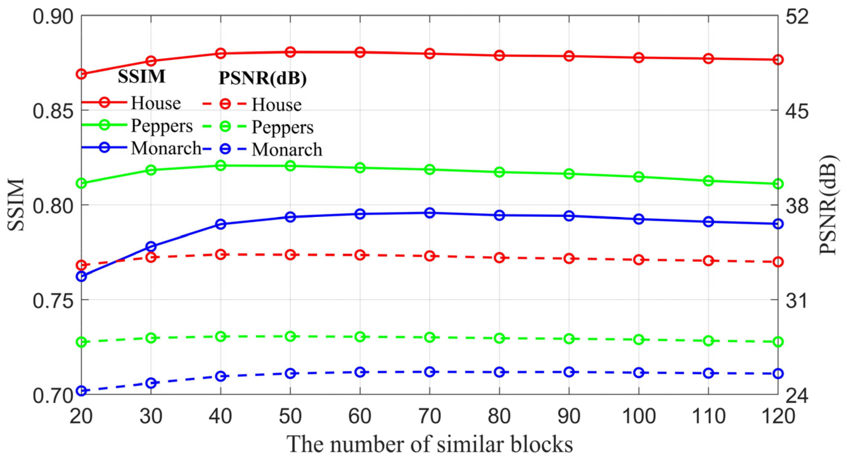
4.1. The Model Parameters Setting
4.2. The Effect of Group Sparse Coefficient Regularization Constraint
4.3. Data Results
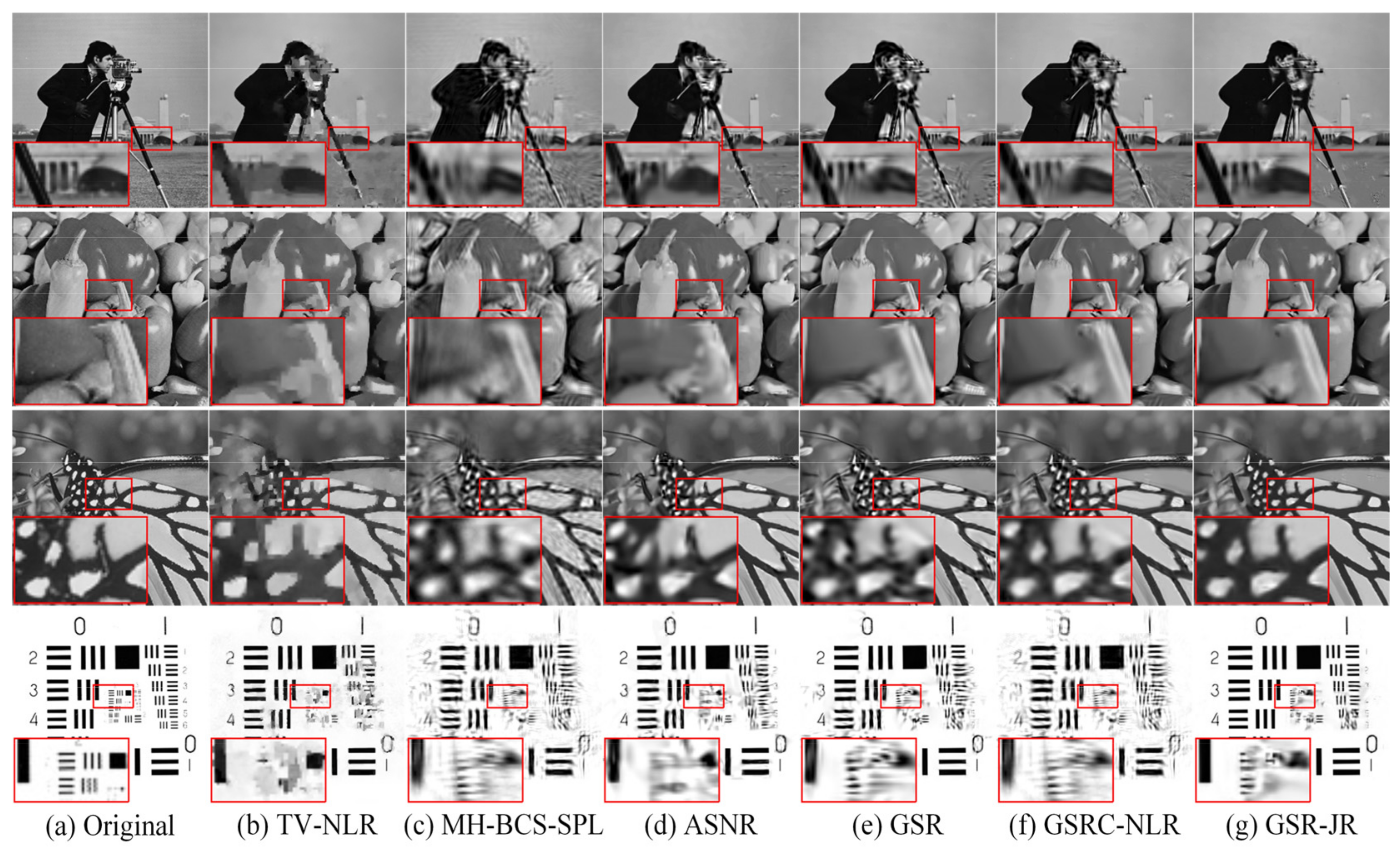
4.4. Visual Effects
4.5. Reconstruction Time
5. Conclusions
Author Contributions
Funding
Data Availability Statement
Conflicts of Interest
Appendix A
References
- Donoho, D.L. Compressed sensing. IEEE Trans. Inf. Theory 2006, 52, 1289–1306. [Google Scholar] [CrossRef]
- Candès, E.J.; Romberg, J.; Tao, T. Stable signal recovery from incomplete and inaccurate measurements. Commun. Pure Appl. Math. 2006, 59, 1207–1223. [Google Scholar] [CrossRef] [Green Version]
- Candès, E.J.; Romberg, J. Sparsity and incoherence in compressive sampling. Inverse Probl. 2007, 23, 969–985. [Google Scholar] [CrossRef] [Green Version]
- Nyquist, H. Certain Topics in Telegraph Transmission Theory. Proc. IEEE 1928, 47, 617–644. [Google Scholar] [CrossRef]
- Monin, S.; Hahamovich, E.; Rosenthal, A. Single-pixel imaging of dynamic objects using multi-frame motion estimation. Sci. Rep. 2021, 11, 7712. [Google Scholar] [CrossRef]
- Zheng, L.; Brian, N.; Mitra, S. Fast magnetic resonance imaging simulation with sparsely encoded wavelet domain data in a compressive sensing framework. J. Electron. Imaging 2013, 22, 57–61. [Google Scholar] [CrossRef] [Green Version]
- Tello Alonso, M.T.; Lopez-Dekker, F.; Mallorqui, J.J. A Novel Strategy for Radar Imaging Based on Compressive Sensing. IEEE Trans. Geosci. Remote Sens. 2010, 48, 4285–4295. [Google Scholar] [CrossRef] [Green Version]
- Liu, J.; Huang, K.; Yao, X. Common-innovation subspace pursuit for distributed compressed sensing in wireless sensor networks. IEEE Sens. J. 2019, 19, 1091–1103. [Google Scholar] [CrossRef]
- Courot, A.; Cabrera, D.; Gogin, N.; Gaillandre, L.; Lassau, N. Automatic cervical lymphadenopathy segmentation from CT data using deep learning. Diagn. Interv. Imaging 2021, 102, 675–681. [Google Scholar] [CrossRef] [PubMed]
- Markel, V.A.; Mital, V.; Schotland, J.C. Inverse problem in optical diffusion tomography. III. Inversion formulas and singular-value decomposition. J. Opt. Soc. Am. 2003, 20, 890–902. [Google Scholar] [CrossRef] [Green Version]
- Wiskin, J.; Malik, B.; Natesan, R.; Lenox, M. Quantitative assessment of breast density using transmission ultrasound tomography. Med. Phys. 2019, 46, 2610–2620. [Google Scholar] [CrossRef] [Green Version]
- Kiesel, P.; Alvarez, V.G.; Tsoy, N.; Maraspini, R.; Gorilak, P.; Varga, V.; Honigmann, A.; Pigino, G. The molecular structure of mammalian primary cilia revealed by cryo-electron tomography. Nat. Struct. Mol. Biol. 2020, 27, 1115–1124. [Google Scholar] [CrossRef]
- Vasin, V.V. Relationship of several variational methods for the approximate solution of ill-posed problems. Math. Notes Acad. Sci. USSR 1970, 7, 161–165. [Google Scholar] [CrossRef]
- Candes, E.J.; Romberg, J.; Tao, T. Robust uncertainty principles: Exact signal reconstruction from highly incomplete frequency information. IEEE Trans. Inf. Theory 2006, 52, 489–509. [Google Scholar] [CrossRef] [Green Version]
- Zenzo, S.D. A note on the gradient of a multi-image. Comput. Vis. Graph. Image Processing 1986, 33, 116–125. [Google Scholar] [CrossRef]
- Zhang, J.; Liu, S.; Zhao, D.; Xiong, R.; Ma, S. Improved total variation based image compressive sensing recovery by nonlocal regularization. In Proceedings of the 2013 IEEE International Symposium on Circuits and Systems (ISCAS), Beijing, China, 19–23 May 2013; pp. 2836–2839. [Google Scholar] [CrossRef]
- Wang, S.; Liu, Z.W.; Dong, W.S.; Jiao, L.C.; Tang, Q.X. Total variation based image deblurring with nonlocal self-similarity constraint. Electron. Lett. 2011, 47, 916–918. [Google Scholar] [CrossRef]
- Buades, A.; Coll, B.; Morel, J.M. A non-local algorithm for image denoising. In Proceedings of the IEEE Computer Society Conference on Computer Vision and Pattern Recognition, San Diego, CA, USA, 20–25 June 2005; Volume 2, pp. 60–65. [Google Scholar] [CrossRef]
- Gan, L. Block Compressed Sensing of Natural Images. In Proceedings of the 2007 15th International Conference on Digital Signal Processing, Wales, UK, 1–4 July 2007; pp. 403–406. [Google Scholar] [CrossRef]
- Chen, C.; Tramel, E.W.; Fowler, J.E. Compressed-sensing recovery of images and video using multi hypothesis predictions. In Proceedings of the 2011 Conference Record of the Forty Fifth Asilomar Conference on Signals, Systems and Computers (ASILOMAR), Pacific Grove, CA, USA, 6–9 November 2011; pp. 1193–1198. [Google Scholar] [CrossRef]
- Zha, Z.; Liu, X.; Zhang, X.; Chen, Y.; Tang, L.; Bai, Y.; Wang, Q.; Shang, Z. Compressed sensing image reconstruction via adaptive sparse nonlocal regularization. Vis. Comput. 2018, 34, 117–137. [Google Scholar] [CrossRef]
- Yang, J.; Wright, J.; Huang, T.S.; Ma, Y. Image Super-Resolution Via Sparse Representation. IEEE Trans. Image Processing 2010, 19, 2861–2873. [Google Scholar] [CrossRef] [PubMed]
- Manzo, M. Attributed Relational SIFT-Based Regions Graph: Concepts and Applications. Mach. Learn. Knowl. Extr. 2020, 3, 233–255. [Google Scholar] [CrossRef]
- Zhang, J.; Zhao, D.; Gao, W. Group-based Sparse Representation for Image Restoration. IEEE Trans. Image Processing 2014, 23, 3336–3351. [Google Scholar] [CrossRef] [Green Version]
- Zha, Z.; Zhang, X.; Wang, Q.; Tang, L.; Liu, X. Group-based Sparse Representation for Image Compressive Sensing Reconstruction with Non-Convex Regularization. Neurocomputing 2017, 296, 55–63. [Google Scholar] [CrossRef] [Green Version]
- Zha, Z.; Zhang, X.; Wu, Y.; Wang, Q.; Liu, X.; Tang, L.; Yuan, X. Non-Convex Weighted Lp Nuclear Norm based ADMM Framework for Image Restoration. Neurocomputing 2018, 311, 209–224. [Google Scholar] [CrossRef]
- Zhao, F.; Fang, L.; Zhang, T.; Li, Z.; Xu, X. Image compressive sensing reconstruction via group sparse representation and weighted total variation. Syst. Eng. Electron. Technol. 2020, 42, 2172–2180. Available online: https://www.sys-ele.com/CN/10.3969/j.issn.1001-506X.2020.10.04 (accessed on 6 December 2021).
- Keshavarzian, R.; Aghagolzadeh, A.; Rezaii, T. LLp norm regularization based group sparse representation for image compressed sensing recovery. Signal Processing: Image Commun. 2019, 78, 477–493. [Google Scholar] [CrossRef]
- Zha, Z.; Yuan, X.; Wen, B.; Zhou, J.; Zhu, C. Group Sparsity Residual Constraint with Non-Local Priors for Image Restoration. IEEE Trans. Image Processing 2020, 29, 8960–8975. [Google Scholar] [CrossRef]
- Zha, Z.; Liu, X.; Zhou, Z.; Huang, X.; Shi, J.; Shang, Z.; Tang, L.; Bai, Y.; Wang, Q.; Zhang, X. Image denoising via group sparsity residual constraint. In Proceedings of the 2017 IEEE International Conference on Acoustics, Speech and Signal Processing (ICASSP), New Orleans, LA, USA, 5–9 March 2017; pp. 1787–1791. [Google Scholar] [CrossRef] [Green Version]
- Boyd, S. Distributed Optimization and Statistical Learning via the Alternating Direction Method of Multipliers. Found. Trends Mach. Learn. 2010, 3, 1–122. [Google Scholar] [CrossRef]
- Daubechies, I.; Defrise, M.; Mol, C.D. An iterative thresholding algorithm for linear inverse problems with a sparsity constraint. Commun. Pure Appl. Math. 2010, 57, 1413–1457. [Google Scholar] [CrossRef] [Green Version]
- Avcibas, I.; Sankur, B.; Sayood, K. Statistical evaluation of image quality measures. J. Electron. Imaging 2002, 11, 206–223. [Google Scholar] [CrossRef] [Green Version]
- Zhou, W.; Bovik, A.C.; Sheikh, H.R.; Simoncelli, E.P. Image quality assessment: From error visibility to structural similarity. IEEE Trans. Image Processing 2004, 13, 600–612. [Google Scholar] [CrossRef] [Green Version]
- Chang, S.G.; Yu, B.; Vetterli, M. Adaptive wavelet thresholding for image denoising and compression. IEEE Trans. Image Processing 2000, 9, 1532–1546. [Google Scholar] [CrossRef] [Green Version]
- Mallat, S.G.; Zhang, Z. Matching Pursuits with Time-Frequency Dictionaries. IEEE Trans. Signal Processing 1993, 41, 3397–3415. [Google Scholar] [CrossRef] [Green Version]


| Regularization Constraint | With Group Sparse Coefficient Regularization | Without Group Sparse Coefficient Regularization | ||||
|---|---|---|---|---|---|---|
| Image | PSNR | SSIM | Time | PSNR | SSIM | Time |
| House | 34.30 | 0.880 | 692.50 | 34.14 | 0.8770 | 1746.53 |
| Peppers | 28.26 | 0.8196 | 796.02 | 28.17 | 0.8189 | 2098.52 |
| Monarch | 27.60 | 0.8910 | 1291.21 | 26.94 | 0.8887 | 2102.25 |
| Airplane | 25.91 | 0.8405 | 1227.76 | 25.62 | 0.8393 | 2093.47 |
| Images | Methods | Sensing Rates | ||||
|---|---|---|---|---|---|---|
| R = 0.1 | R = 0.15 | R = 0.2 | R = 0.25 | R = 0.3 | ||
| PSNR|SSIM | PSNR|SSIM | PSNR|SSIM | PSNR|SSIM | PSNR|SSIM | ||
| Cameraman | TV-NLR | 22.98|0.7498 | 24.51|0.7973 | 25.76|0.8295 | 27.38|0.8603 | 27.99|0.8746 |
| MH-BCS-SPL | 22.13|0.6791 | 24.37|0.7664 | 25.88|0.8111 | 27.16|0.8408 | 28.08|0.8607 | |
| ASNR | 23.76|0.7802 | 26.17|0.8377 | 27.75|0.8668 | 28.87|0.8889 | 29.96|0.9037 | |
| GSR | 22.90|0.7680 | 25.50|0.8309 | 27.17|0.8627 | 28.40|0.8847 | 29.62|0.9041 | |
| GSRC-NLR | 23.79|0.7778 | 26.38|0.8387 | 27.19|0.8575 | 28.62|0.8833 | 29.66|0.9021 | |
| GSR-JR | 24.57|0.7938 | 26.62|0.8408 | 28.16|0.8702 | 29.15|0.8914 | 30.19|0.9073 | |
| House | TV-NLR | 29.55|0.8326 | 31.55|0.8604 | 33.18|0.8819 | 34.39|0.8969 | 35.48|0.9104 |
| MH-BCS-SPL | 30.28|0.8357 | 32.49|0.8736 | 33.84|0.8934 | 34.95|0.9029 | 35.69|0.9186 | |
| ASNR | 33.60|0.8836 | 35.79|0.9079 | 36.97|0.9250 | 38.12|0.9407 | 39.06|0.9503 | |
| GSR | 33.75|0.8807 | 35.88|0.9121 | 37.31|0.9322 | 38.36|0.9451 | 39.29|0.9539 | |
| GSRC-NLR | 34.07|0.8794 | 35.77|0.9065 | 37.11|0.9276 | 38.36|0.9443 | 39.30|0.9539 | |
| GSR-JR | 34.30|0.8805 | 35.71|0.9031 | 37.04|0.9239 | 38.29|0.9415 | 39.13|0.9506 | |
| Peppers | TV-NLR | 25.72|0.7624 | 27.72|0.8105 | 29.04|0.8418 | 30.13|0.8630 | 30.70|0.8752 |
| MH-BCS-SPL | 25.16|0.7187 | 27.44|0.7874 | 28.61|0.8157 | 29.63|0.8405 | 30.20|0.8513 | |
| ASNR | 27.50|0.8030 | 29.74|0.8490 | 30.91|0.8700 | 32.33|0.8919 | 33.28|0.9050 | |
| GSR | 26.93|0.7944 | 29.30|0.8411 | 30.83|0.8693 | 32.11|0.8890 | 33.02|0.9028 | |
| GSRC-NLR | 27.88|0.8134 | 29.92|0.8514 | 30.97|0.8696 | 32.17|0.8883 | 32.94|0.9003 | |
| GSR-JR | 28.26|0.8196 | 30.13|0.8557 | 31.51|0.8793 | 32.61|0.8953 | 33.48|0.9075 | |
| Starfish | TV-NLR | 22.84|0.6709 | 24.40|0.7476 | 25.73|0.7991 | 26.52|0.8314 | 28.33|0.8739 |
| MH-BCS-SPL | 22.54|0.6843 | 24.78|0.7617 | 25.93|0.7972 | 26.96|0.8289 | 27.90|0.8506 | |
| ASNR | 24.33|0.7554 | 27.22|0.8392 | 29.66|0.8909 | 31.77|0.9229 | 33.15|0.9387 | |
| GSR | 23.60|0.7344 | 26.99|0.8400 | 29.41|0.8901 | 31.38|0.9186 | 33.00|0.9375 | |
| GSRC-NLR | 24.41|0.7614 | 27.20|0.8408 | 28.24|0.8703 | 29.86|0.9028 | 31.37|0.9256 | |
| GSR-JR | 25.65|0.7952 | 28.20|0.8588 | 30.26|0.8997 | 32.02|0.9268 | 33.58|0.9415 | |
| Monarch | TV-NLR | 23.01|0.7726 | 25.66|0.8484 | 27.16|0.8832 | 29.24|0.9128 | 29.73|0.9239 |
| MH-BCS-SPL | 23.19|0.7575 | 25.64|0.8383 | 27.10|0.8660 | 28.25|0.8856 | 29.20|0.9005 | |
| ASNR | 25.86|0.8703 | 28.97|0.9194 | 31.88|0.9475 | 33.46|0.9595 | 34.78|0.9670 | |
| GSR | 25.29|0.8640 | 28.22|0.9179 | 30.77|0.9433 | 32.79|0.9578 | 34.25|0.9659 | |
| GSRC-NLR | 26.33|0.8795 | 29.01|0.9227 | 30.32|0.9388 | 32.15|0.9540 | 33.43|0.9626 | |
| GSR-JR | 27.60|0.8910 | 29.95|0.9270 | 32.05|0.9483 | 33.75|0.9613 | 35.06|0.9680 | |
| Airplane | TV-NLR | 23.44|0.7568 | 25.32|0.8197 | 26.81|0.8646 | 28.33|0.8917 | 28.79|0.9018 |
| MH-BCS-SPL | 23.67|0.7638 | 25.44|0.8199 | 27.19|0.8525 | 28.59|0.8870 | 29.67|0.8945 | |
| ASNR | 25.13|0.8248 | 27.35|0.8764 | 29.10|0.9065 | 30.50|0.9253 | 32.15|0.9432 | |
| GSR | 24.57|0.8219 | 26.56|0.8703 | 28.96|0.9086 | 30.48|0.9283 | 32.03|0.9440 | |
| GSRC-NLR | 25.36|0.8335 | 27.54|0.8819 | 28.93|0.9070 | 30.49|0.9280 | 31.91|0.9432 | |
| GSR-JR | 25.91|0.8405 | 28.19|0.8897 | 29.98|0.9173 | 31.35|0.9361 | 32.70|0.9475 | |
| Parrot | TV-NLR | 24.60|0.8273 | 25.93|0.8599 | 27.29|0.8852 | 28.21|0.9005 | 29.16|0.9139 |
| MH-BCS-SPL | 25.34|0.8219 | 27.36|0.8749 | 29.23|0.8975 | 30.08|0.9133 | 31.01|0.9254 | |
| ASNR | 26.73|0.8707 | 28.44|0.8977 | 30.38|0.9189 | 31.46|0.9314 | 33.12|0.9420 | |
| GSR | 26.34|0.8747 | 28.97|0.9075 | 31.16|0.9247 | 32.36|0.9331 | 33.82|0.9472 | |
| GSRC-NLR | 27.35|0.8815 | 29.52|0.9079 | 30.74|0.9221 | 31.49|0.9331 | 32.41|0.9427 | |
| GSR-JR | 27.66|0.8805 | 29.84|0.9073 | 31.54|0.9237 | 32.16|0.9355 | 33.73|0.9450 | |
| Man | TV-NLR | 23.49|0.6363 | 24.77|0.7067 | 26.05|0.7584 | 27.32|0.8077 | 27.85|0.8274 |
| MH-BCS-SPL | 23.00|0.5746 | 24.44|0.6534 | 25.36/0.6959 | 26.44|0.7451 | 27.36|0.7811 | |
| ASNR | 24.16|0.6800 | 26.08|0.7636 | 27.55|0.8195 | 28.55|0.8499 | 29.81|0.8786 | |
| GSR | 23.80|0.6658 | 25.80|0.7602 | 27.440.8182 | 28.71|0.8551 | 29.81|0.8836 | |
| GSRC-NLR | 24.42|0.6900 | 26.29/0.7686 | 27.61/0.8180 | 28.86|0.8538 | 29.80|0.8804 | |
| GSR-JR | 24.91|0.6957 | 26.64|0.7695 | 28.06|0.8206 | 29.22|0.8582 | 30.45|0.8846 | |
| Resolution chart | TV-NLR | 20.66|0.8802 | 25.05|0.9470 | 28.72|0.9710 | 32.29|0.9811 | 36.05|0.9880 |
| MH-BCS-SPL | 17.69|0.6482 | 20.32|0.7626 | 22.75|0.8600 | 25.12|0.9051 | 27.10|0.9330 | |
| ASNR | 20.68|0.8636 | 25.95|0.9560 | 30.07|0.9785 | 32.70|0.9861 | 36.88|0.9911 | |
| GSR | 20.20|0.8489 | 26.03|0.9562 | 30.16|0.9764 | 36.28|0.9890 | 38.07|0.9912 | |
| GSRC-NLR | 20.26|0.8268 | 25.37|0.9427 | 25.55|0.9390 | 29.49|0.9733 | 31.83|0.9826 | |
| GSR-JR | 25.12|0.9466 | 31.99|0.9818 | 35.07|0.9889 | 34.65|0.9903 | 41.63|0.9953 | |
| Camera test | TV-NLR | 15.72|0.6992 | 19.10|0.8330 | 21.74|0.9007 | 23.93|0.9434 | 22.32|0.8614 |
| MH-BCS-SPL | 19.63|0.7416 | 22.25|0.8074 | 24.04|0.8428 | 26.09|0.8864 | 27.68|0.9025 | |
| ASNR | 24.14|0.9578 | 28.23|0.9859 | 32.03|0.9919 | 34.62|0.9944 | 36.78|0.9954 | |
| GSR | 24.47|0.9658 | 29.00|0.9856 | 32.52|0.9913 | 35.05|0.9937 | 36.42|0.9937 | |
| GSRC-NLR | 24.34|0.9579 | 28.51|0.9852 | 29.43|0.9861 | 32.45|0.9935 | 34.84|0.9956 | |
| GSR-JR | 25.87|0.9734 | 29.98|0.9888 | 33.30|0.9936 | 35.40|0.9956 | 37.83|0.9966 | |
Publisher’s Note: MDPI stays neutral with regard to jurisdictional claims in published maps and institutional affiliations. |
© 2022 by the authors. Licensee MDPI, Basel, Switzerland. This article is an open access article distributed under the terms and conditions of the Creative Commons Attribution (CC BY) license (https://creativecommons.org/licenses/by/4.0/).
Share and Cite
Wang, R.; Qin, Y.; Wang, Z.; Zheng, H. Group-Based Sparse Representation for Compressed Sensing Image Reconstruction with Joint Regularization. Electronics 2022, 11, 182. https://doi.org/10.3390/electronics11020182
Wang R, Qin Y, Wang Z, Zheng H. Group-Based Sparse Representation for Compressed Sensing Image Reconstruction with Joint Regularization. Electronics. 2022; 11(2):182. https://doi.org/10.3390/electronics11020182
Chicago/Turabian StyleWang, Rongfang, Yali Qin, Zhenbiao Wang, and Huan Zheng. 2022. "Group-Based Sparse Representation for Compressed Sensing Image Reconstruction with Joint Regularization" Electronics 11, no. 2: 182. https://doi.org/10.3390/electronics11020182