Article

Wireless Communication Channel Scenarios: Machine-Learning-Based Identification and Performance Enhancement

College of Engineering and Technology, Arab Academy for Science, Technology and Maritime Transport, Alexandria 1029, Egypt
*
Author to whom correspondence should be addressed.
Electronics 2022, 11(19), 3253; https://doi.org/10.3390/electronics11193253
Submission received: 7 September 2022 / Revised: 28 September 2022 / Accepted: 2 October 2022 / Published: 10 October 2022
(This article belongs to the Special Issue 5G Mobile Telecommunication Systems and Recent Advances)

Abstract

:
Wireless communication channel scenario classification is crucial for new modern wireless technologies. Reducing the time consumed by the data preprocessing phase for such identification is also essential, especially for multiple-scenario transitions in 6G. Machine learning (ML) has been used for scenario identification tasks. In this paper, the least absolute shrinkage and selection operator (LASSO) is used instead of ElasticNet in order to reduce the computational time of data preprocessing for ML. Moreover, the computational time and performance of different ML models are evaluated based on a regularization technique. The obtained results reveal that the LASSO operator achieves the same feature selection performance as ElasticNet; however, the LASSO operator consumes less computational time. The achieved run time of LASSO is 0.33 s, while the ElasticNet corresponding value is 0.67 s. The identification for each specific class for K-Nearest Neighbor (KNN), Support Vector Machine (SVM), and k-Means and Gaussian Mixture Model (GMM) is evaluated using Receiver Operating Characteristics (ROC) curves and Area Under the Curve (AUC) scores. The KNN algorithm has the highest class-average AUC score at 0.998, compared to SVM, k-Means, and GMM with values of 0.994, 0.983, and 0.989, respectively. The GMM is the fastest algorithm among others, having the lowest classification time at 0.087 s, compared to SVM, k-Means, and GMM with values of 0.155, 0.26, and 0.087, respectively.

1. Introduction

It is widely known that artificial intelligence (AI) has become an essential addition to industries related to wireless communications. The data obtained from the surrounding environment are huge in volume, as the number of smart devices is increasing—especially in industry, scientific, and medical domains [1,2]. Connecting rural and distant locations has become crucial for future networks due to the rise in global communication needs and the growth of the Internet of Things [3]. As the variety of smartphones, laptops, tablets, and data-driven sensors are all typical data transceiver devices, their data can be and are processed by AI. The main functionality of AI is to train algorithms to make decisions and take actions. ML is a subset of AI in which large amounts of data are used in training an ML algorithm to allow it to learn more about the processed information [4]. Once the ML algorithm is trained on the training data, it can successfully make predictions or decisions with new data and execute tasks using inferential statistics and arithmetic calculations. This can permit and facilitate ML modeling for wireless communication system availability, mobility accessibility, cross-communication management, and the optimization of automated networks based on 6G data. The aim is to ensure that the key performance indicators are meeting the quality-of-service (QoS) requirements. It is anticipated that the 6G network will offer diverse services and seamless network coverage for everyone and everything. The integrated satellite–terrestrial network design combines the benefits of both satellite and terrestrial networks. The current promises are to provide worldwide broadband connectivity for all sorts of users [5,6,7,8]. It has attracted much interest from both academia and business.
A wireless communication system mainly consists of a physical layer, a middle layer, and an end-user layer, as shown in Figure 1. Each layer requires different AI approaches to enhance the QoS, system security, privacy, latency, power allocation and control, and channel capacity [9].
The main concern of the use of ML in the physical layer is the channel encoding, decoding, and estimation. One of these ML applications is scenario classification, which can be regarded as channel estimation. A scenario for a wireless channel is defined as the specific channel environment of data transmission [9]. For example, rural, suburban, urban, and indoor hotspots and satellites are all typical scenarios. The rural macro-cell (RMa) and the urban macro-cell (UMa) are two typical different scenarios. The UMa is deployed in urban areas as it indicates a city or a town, while the term RMa is used for rural areas or countries with smaller populations and less scattering.
In some cases, a number of circumstances or scenarios regularly occur. Users that use high-speed transportation, such as high-speed railways, may attest to this. As the user navigates across a variety of possible scenarios, including deserts, mountains, stations, and other impediments, the user places substantial strain on existing communication systems. Therefore, accurately defining wireless channel scenarios is important for meeting user QoS needs. However, the traditional forms of statistics in radio propagation, such as the Okumura and Hata models, were introduced under the assumption that the propagation model of the scenario was previously known, such as in urban scenarios [10]. This can lead to certain inaccurate classifications or mistakes. In response, minimizing complexities and run times and precisely identifying the scenario task are crucial for increasing communication system reliability. Moreover, the power efficiency, beam management, maintenance, bandwidth allocation efficiency, network setup, operation, throughput, QoS prediction, and coverage performance can be tackled by AI-based solutions. Deep-learning methods are usually used in solving complex problems, but require more computational time. The extraction of elevation and azimuth angles from CIR to distinguish the NLoS and LoS scenarios in urban places was performed in [11]. Also, an accurate classification performance was achieved using convolutional networks in the problem of fingerprint feature extraction and classification [12]. The authors of [13] demonstrated via their ML approaches that supervised classification algorithms and unsupervised learning clustering algorithms can be effective classification strategies for scenario identification.
In a previous work [14], we introduced an enhanced feature-selection process based on the regularization concept to enhance the classification performance of [14] and reduced the computational complexity of the ML algorithms with high generalization ability. The authors of [15] initiated the problem formulation of classification of typical terrestrial scenarios. However, the latency of transition and classification was not their concern. Therefore, to iterate upon their results, the time consumption of the preprocessing workflow and ML classification time are crucial issues to address. Minimizing the preprocessing procedure computations and the classification time of the algorithm are required to have quick scenario identification when a transition between multiple scenarios occurs. The ROC curve is important as an evaluation parameter as it contains both true positive rate (TPR) and false positive rate (FPR). The main motivation for this work is enhancing recent work [14,15] in terms of preprocessing time and performance of the wireless communication scenario identification. The proposed method has considered the latency of the classification scheme.
Hence, this paper contributes the following:
  • Reduction of the model response and latency for the preprocessing workflow of each regularization technique instruction used in the previous model [14]. The previous model adopted ElasticNet without studying the time consumption. In this work, the performance and time efficiency results prove that adopting the LASSO is more suitable than ElasticNet. It achieves the same feature-selection performance of ElasticNet but in much less time.
  • Calculation of the classification time of KNN, SVM, k-Means, and GMM. The training phase and testing phase runtimes are computed and compared for both supervised algorithms (KNN and SVM). The formulation of clusters and the “fit and predict” runtime for the unsupervised learning k-Means and GMM are revealed.
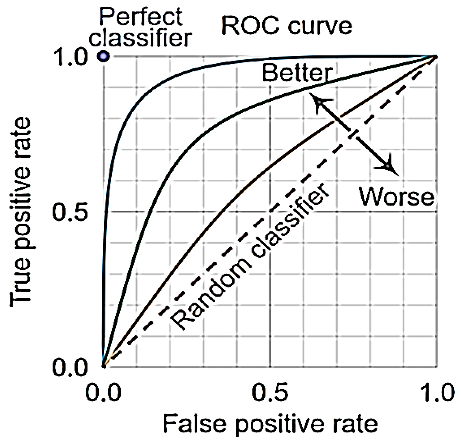
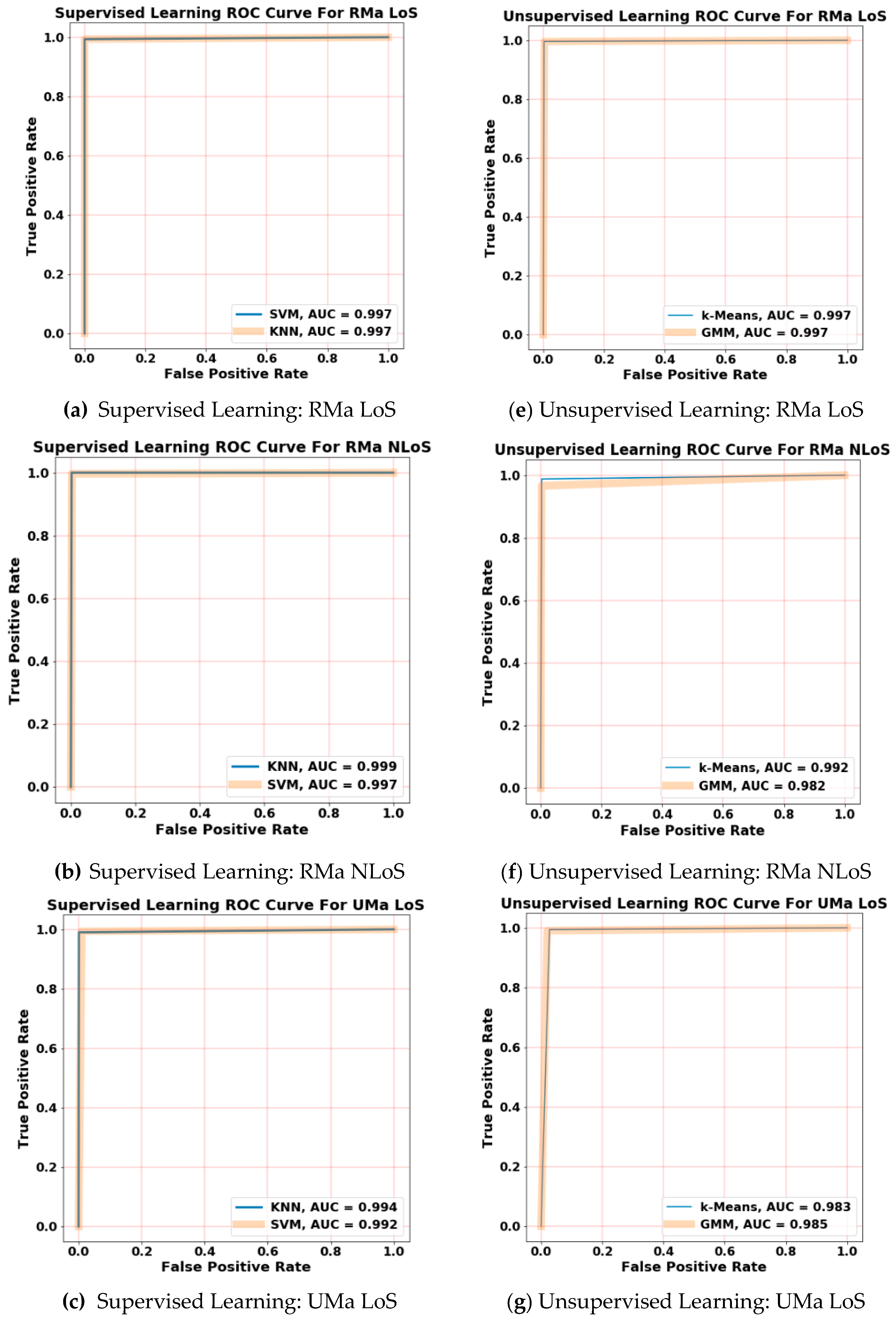
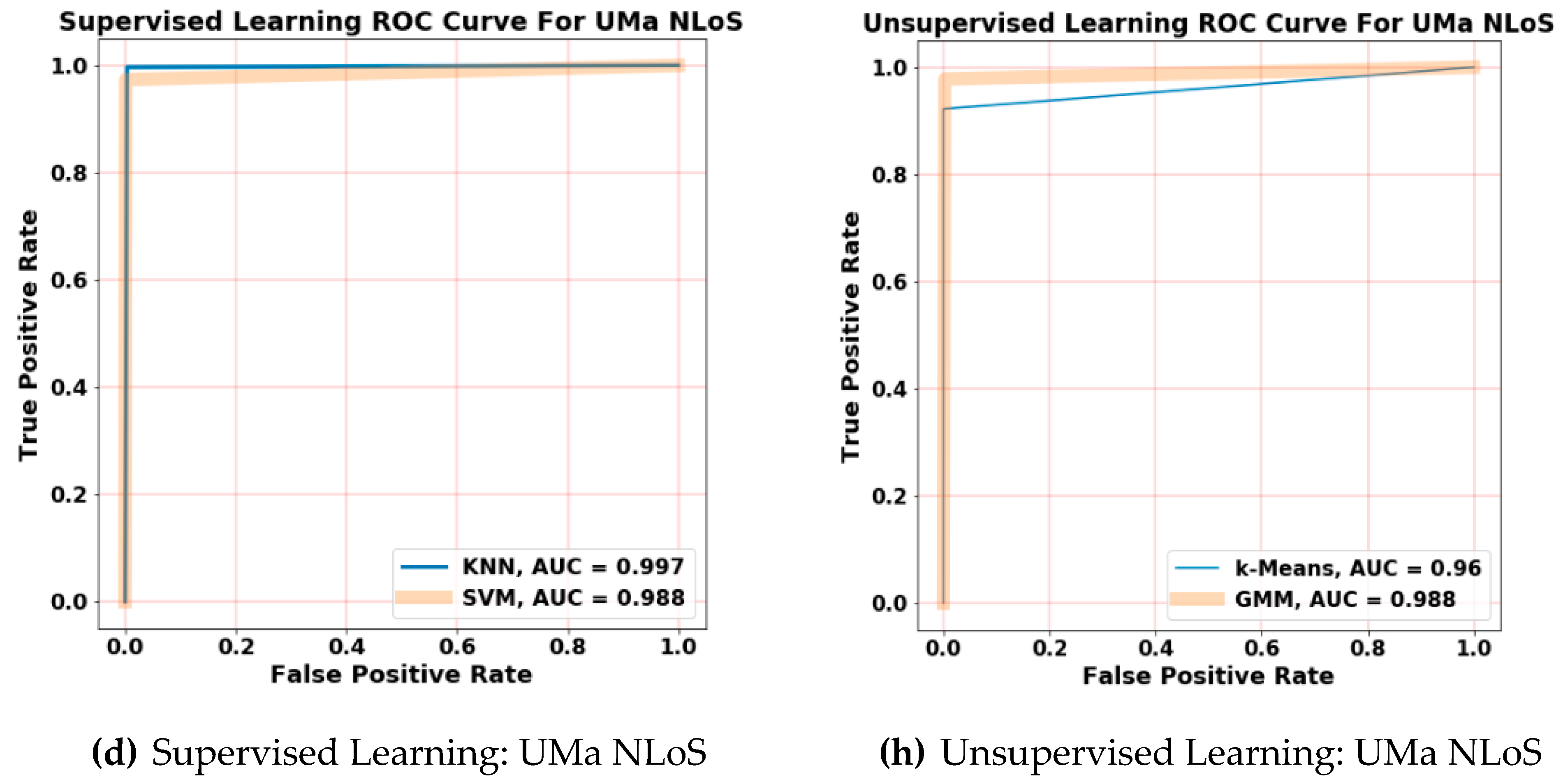
  • Calculation and study of the ROC curves and AUC scores for each class in each model. Both ROC curves and AUC scores of the classes are calculated as one over all, where the evaluation is taken as a binary such that every class is distinguished from the others (e.g., the RMa LoS represented as ‘1’ versus the other classes presented as ‘0’).
The rest of this paper is organized as follows. Section 2 provides information about the dataset used in this research, the model specification, and preprocessing and processing procedures. Section 3 shows the results and discussion of the preprocessing and classification phases, including time and ROC curves. Section 4 is devoted to the main conclusions.

2. Model Planning Procedures

In this section, the dataset adopted in this work is discussed. The features that are preprocessed describe each wireless communication scenario, such as delay spread ( D σ ), path loss ( P L ), k-factor ( K F ), elevation spread angle of arrival ( σ E o A ), elevation spread angle of departure ( σ E o D ), azimuth spread angle of arrival ( σ A o A ), and azimuth spread angle of departure ( σ A o D ). In addition, this section introduces the preprocessing procedure and the methods of evaluation.

2.1. Dataset Origination and Parameters

The dataset is taken from [14], where each scenario parameter is validated through the 3GPP standard. These parameters describe the large-scale fading and small-scale fading parameters such as D σ , P L , K F , σ E o A , σ E o D , σ A o A , and σ A o D . The angular information is extracted from CIR using the space-alternating generalized expectation-maximization algorithm in MIMO model using 31 antenna elements [14,15]. The CIR snapshots are generated from the reception of the signal from mobile terminal (MT) to base station (BS). These CIR snapshots are supposed to be processed from the BS end as shown in Figure 2.
The NLoS and the LoS cases are obtained for both RMa and UMa, so the number of classes is four. As mentioned before, the UMa scenario is specified in urban places as it refers to a town or a city, while the RMa is defined for rural areas such as towns that have small population and reduced scattering.
P L is defined as a decrease of power due to a distance. It is the relation between the distance d and the actual path loss, denoted as P L ( d 0 ) , in a unique scenario and is expressed as P d B [16]:
P d B = P L ( d 0 ) + 10   γ   l o g 10 ( d d 0 ) + S σ [ d B ] ,
where the P L exponent is defined as γ, d 0 is the reference distance, and S σ [ d B ] represents the standard normal distribution.
K F is an essential small scale fading (SSF) parameter. It is the ratio between the power of a dominant LoS component and the NLoS multipath components. At every CIR snapshot capture, the K F ( K d B ) can be denoted as [17]
K d B = 10   l o g { ( | h ( τ m 0 ) | m a x ) 2 τ m τ m 0 ( |   h ( t ) | ) 2 } ,
where τ m represents the current period of the m th component delay, the highest amplitude occurs at τ m 0 index, and m = 1 , 2 , 3     M . h ( t ) expresses the CIR in time domain. The value of K d B is always greater in LoS scenarios.
D σ is also an important SSF parameter that indicates the channel dispersion of a CIR snapshot in terms of time delay. D σ can be represented as [18]
D σ = Σ m = 1 M   ( τ m τ ¯ )   |   h ( τ m )   | 2 Σ m = 1 M   |   h ( τ m )   | 2 ,
where M denotes the total number of m th components and τ ¯ is the mean excess delay and is denoted as
τ ¯ = Σ m = 1 M τ m   |   h ( τ m )   | 2 Σ m = 1 M   |   h ( τ m )   | 2
The channel capacity is dependant on D σ , where a scenario that has multiple rich scatters will have a larger D σ . Therefore, an NLoS scenario has a higher root mean square (RMS) delay spread (DS).
The angular spread ( σ θ ) denotes the channel dispersion for a CIR snapshot in terms of angular information, where σ θ is obtained as [19]
σ θ = Σ m = 1 M θ m , μ 2 .   |   h ( τ m )   | 2 Σ m = 1 M   |   h ( τ m )   | 2 ,
θ m , μ = m o d ( ( θ m θ ¯ + π , 2 π ) ) π ,
θ ¯ = Σ m = 1 M θ m , μ |   h ( τ m )   | 2 Σ m = 1 M   |   h ( τ m )   | 2 .
The declaration of angle θ is taken for azimuth angle of departure (AoD), azimuth angle of arrival (AoA), elevation angle of departure (EoD), and elevation angle of arrival (EoA). The NLoS scenario has more clusters than the LoS scenario. As a result, the value of σ θ is higher in NLoS scenarios than LoS scenarios.

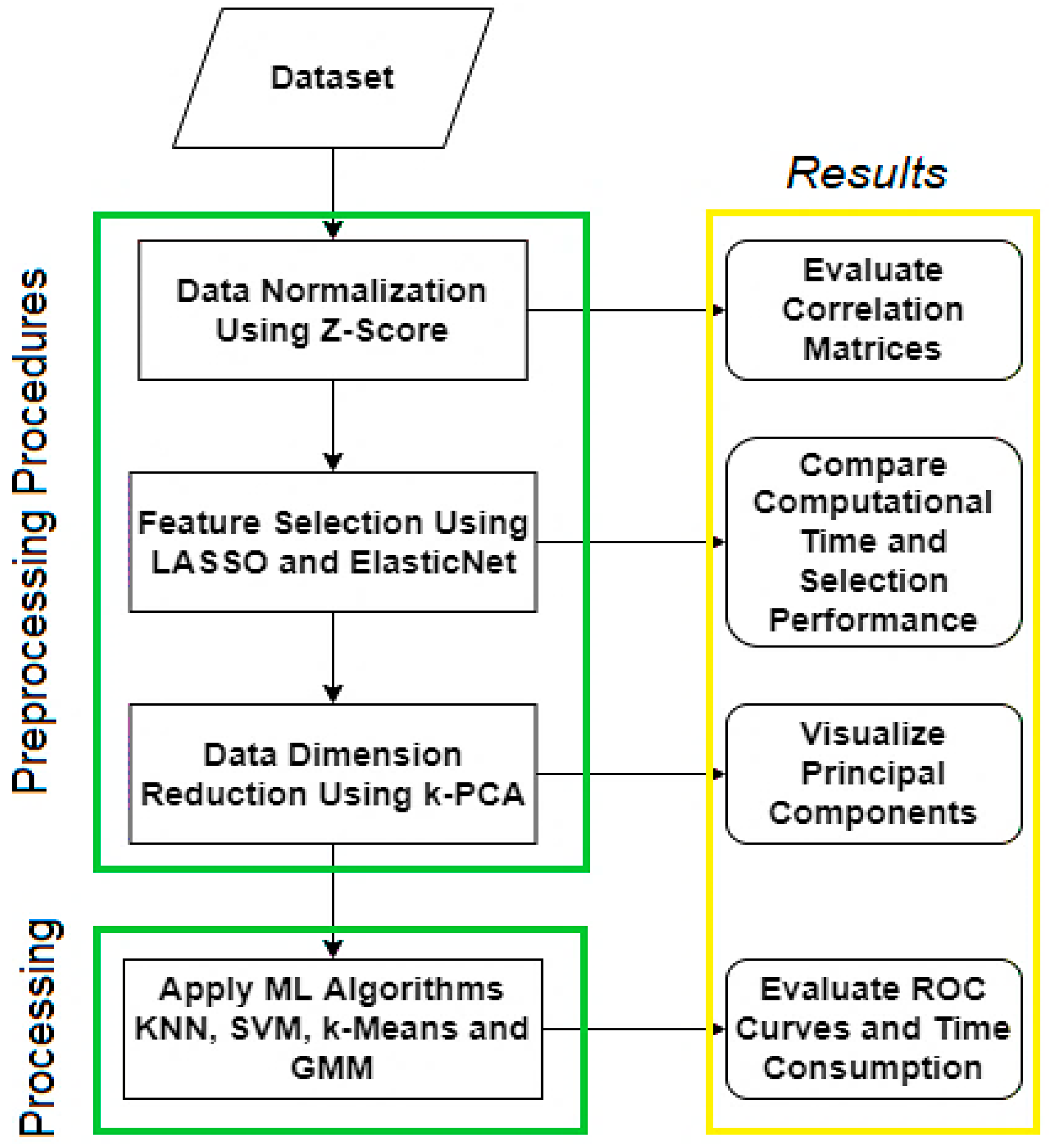
2.2. Preprocessing and Processing Procedures

Figure 3 shows the model planning procedures that represent the flow of the dataset mentioned in the previous section, including the data preprocessing criteria, processing phase, and model evaluation.
The preprocessing procedures are sequential, including normalization, regularization, and dimension reduction. The preliminary dataset enters the preprocessing phase with a data shape of 2000 row and 7 columns, excluding the output label. The dataset can be represented as A   , where A = { D σ , P L , K F , σ E o A , σ E o D , σ A o A , σ A o D , L}, and L represents the outcome label that specifies whether it is Uma LoS, Uma NloS, Rma LoS, or RMa NLoS. Each row, A i , represents a single data point that will be normalized using a Z-score normalization method. The ML models may exhibit bad performance due to the outliers of un-normalized data [16]. The Z-score is applied on each data point A i j , where it represents the distance of a data point to the mean divided by a standard deviation and can be denoted as [20]
A i j = A i j A j ¯ σ A j
where A j ¯ and σ A j are the average and standard deviation of each feature j.
Then, the correlation matrices are used to validate the inter-parameter correlation revealed before normalizing the features and after normalization. The normalized data points are then regularized to drop the unwanted features and to enhance the classification performance [15]. The LASSO operator is L1 regularization type, while the ElasticNet is a combination of both L1 and L2 regularization type. L1 stands for Least Absolute Error, and L2 stands for Least Square Errors [21]. The LASSO regression B ^ l a s s o and ElasticNet regression B ^ e l a s t i c can be denoted, respectively, as
B ^ l a s s o = a r g m i n { 1 2 i = 1 N ( y i β 0 j = 1 p x i j β j ) + λ j = 1 p | β j | }
subject   to   j = 1 p | β j | t
B ^ e l a s t i c = a r g m i n { i 1 2 | y i β 0 j = 1 p x i j β j | 2 2 + λ ( α 1 j = 1 p β j + α 2 j = 1 p β j 2 ) } ,
where both α 1 , α 2 affect the ratio of penalty ( α 1 + α 2 = 1), and λ is the weight of shrinkage. λ expresses the regularization penalty, where 1     λ   0. β 0 is a coefficient with a constant value, while β = ( β 0 ,   β 1 , β 2 , , β N ) is the coefficient vector; t denotes the degree of regularization.
The evaluation of the regularization process is conducted using process runtime and a regularization coefficient evaluation. Here, the runtime was tested on an Intel® Core™ i3-2365M CPU (1.40 GHz) processor using the Python timing library. Once the regularization coefficient of a certain feature obtains 0, t the feature is considered as unwanted noisy data.
The last preprocessing step is the dimension projection. This is used to reduce the number of predictors for the ML, which reflects on the computational complexity reduction [22]. Here, the kernel principal component analysis (k-PCA) is adopted. The kernel type in this paper is a radial basis function (RBF) and can be denoted as
Κ ( A a , A b ) = e x p ( ρ | | A a A b | | 2 ) ,
where A a , A b are two different points and ρ is a hyper-parameter threshold [23]. Then, the output components are visualized as function of probability density function (PDF).
After preprocessing the data, the dimension reduction output is the number of analyzed principal components that are used as ML input predictors. The data are split into training data and validation data. The problem formulation is a classification problem in order to classify between four different scenarios {RMa LoS, RMa NLoS, UMa LoS, UMa NLoS} efficiently. There are two supervised learning algorithms used, KNN and SVM, which require label training. Moreover, two unsupervised learning clustering algorithms are used: k-Means and GMM. The algorithms are then evaluated using ROC curves and their runtime.
The KNN classifies a novel unknown data point based on the majority of the surrounding points based on the nearest distances [24]. The SVM attempts to create different support vectors, then determines the optimal hyper-planes in order to minimize the error and widen the maximal margins for each group of data [25]. The k-Means and GMM are both unsupervised learning methods that create clusters based on the inferential statistics of the data [14].
Each algorithm is then evaluated using the computational time and the ROC curves. The ROC curve shows the relation between the true positive rate and the false positive rate. Figure 4 shows an illustration of an ROC curve [26].
The perfect classification occurs when the area under the curve is maximized. The worst classification occurs when the line becomes straight.

3. Results and Discussion

In this section, the results of each process discussed in the preprocessing and processing procedure are revealed. The correlation matrices of each scenario are discussed before normalization and after using Z-score. The performance and the runtimes of the process of regularization for both LASSO and ElasticNet are compared. The ROC curves of each scenario are discussed for each algorithm. Moreover, the runtime of each algorithm is revealed.

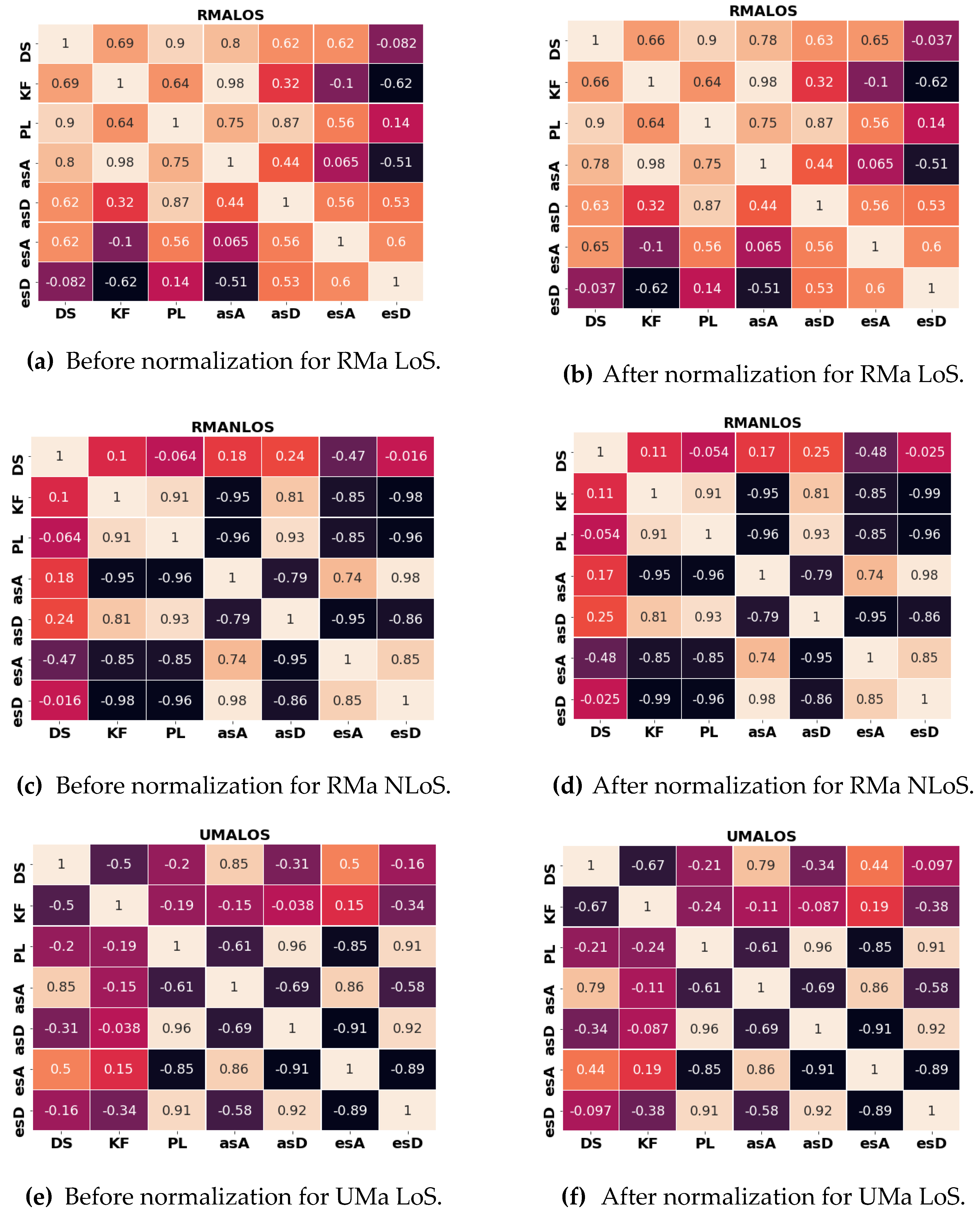
3.1. Z-Score Normalization Impact on Inter-Parameter Correlations

Figure 5 shows the dataset inter-parameter correlations before and after normalization of Z-score for different channel scenarios. The highly positive correlations tend to be bright orange. The highly negative correlations tend to be dark blue. All D σ , P L , K F , σ E o A , σ E o D , σ A o A , and σ A o D are represented as DS, PL, KF, esD, esA, asD, and asA, respectively.
The parts Figure 5a,c,e,g represent the correlation matrices for each scenario before normalizing the features, while the parts Figure 5b,d,f,h display the final result for the correlation after normalization. It is easily noted that the correlation coefficients differences between normalized and un-normalized parameters are negligible as the normalization process only standardizes the data without significantly affecting the inter-parameter correlation. The Z-score keeps the inter-parameter correlations in its region after normalization. The strong, medium, and weak correlations are retained. This determines the robustness of the Z-score and its ability to normalize the data while keeping the data within the correlation region.

3.2. Regularization Evaluation

Table 1 shows the decision of feature elimination for LASSO and ElasticNet, where the elimination is based on the value of the coefficient. If the value is 0, this means that the corresponding feature should be dropped. The decision results of the table are either kept or dropped.
The ElasticNet and LASSO performances are similar. Both have dropped the 0 regularization coefficient parameters esD, asD, and DS. They kept esA, KF, PL, and asA because their coefficients are 0.72, 0.37, 0.25, and 0.12, respectively. These results indicate that the regularization of both LASSO and ElasticNet reduced the data dimensionality from 7 to 4.
Table 2 shows the time evaluation of both LASSO and ElasticNet. The instruction of each one is 10 times and their time average is taken into consideration.
Clearly, the LASSO is more time-efficient and more suitable for this type of dataset as it is a L1 regularization type. The ElasticNet takes more time as it combines both L1 and L2 types during regularization.

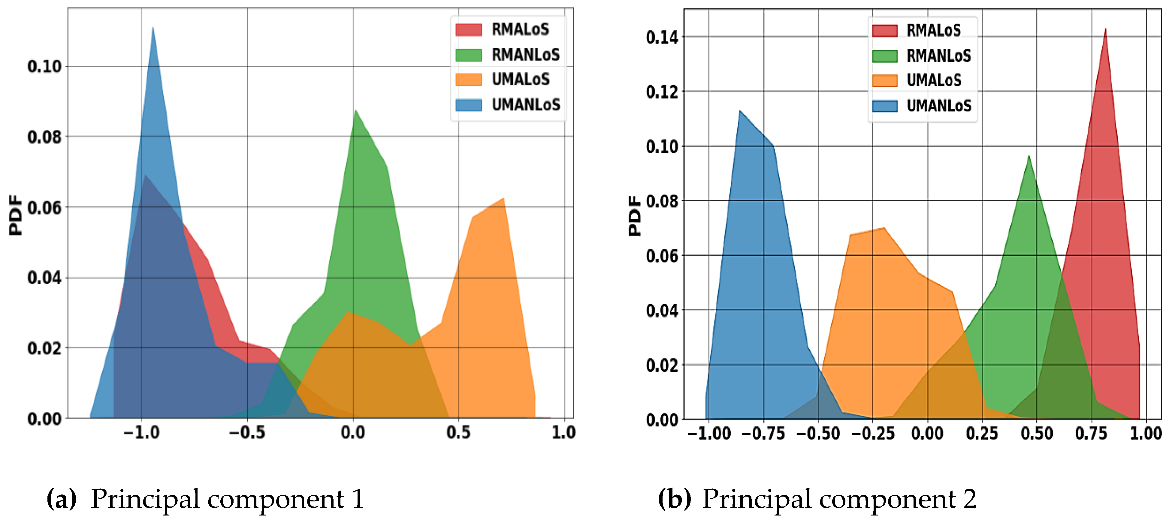
3.3. Dimension Reduction and Data Visualization

As mentioned before, the LASSO reduced the data dimension from 7 to 4 in less time than the ElasticNet. The k-PCA reduces the data dimension even more. The type of kernel is RBF. Figure 6 shows the PDF of the final preprocessed data, where the data have the principal components extracted from k-PCA. Figure 6a shows the PDF of the first principal component, PC1, for all scenarios. The PC1 has an overlay of classes (scenarios). This overlap would cause misclassification due to the overlapped groups. This data overlap can be seen in the cases of RMA NLoS and UMA NLoS. Figure 6b shows the PDF of the second principal component, PC2, which shows a novel differentiation of information that can be used in distinguishing the four classes. In other words, PC2 displays a new dimension of the data: for example, the UMa NLoS can be easily distinguished from RMa LoS. Both PC1 and PC2 components are used as ML predictors.

3.4. ML Evaluation

The ROC curves of each algorithm show a binary classification. Each scenario is compared with the other three scenarios so that it is considered as a binary value of 1 while the other scenarios are represented as 0. Figure 7 shows the ROC curves output for each scenario over the others for all algorithms.
The AUC is the indicator for the binary classification performance. In the case of RMa LoS, all algorithms achieved an AUC score above 0.997. The KNN achieved the highest AUC score in RMa NLoS classification with 0.994. In the case of UMa LoS, the KNN achieved a score of 0.994, outperforming the SVM by 0.02, while the GMM outperformed the k-Means by 0.02. The least AUC score in the case of UMa NLoS was 0.96. which corresponds with the k-Means, while the GMM surpassed the AUC score of k-Means by 0.266. The supervised learning seems to have a better AUC score than unsupervised learning because the TPR and FPR were calculated on the testing set only. The unsupervised learning models were used to cluster the combined dataset (training and validation set). Then, the evaluation was performed by calculating the minimum mean square error of each cluster and comparing it with the actual data output.
The time evaluation for each algorithm is displayed in Table 3. The time of the training and testing were combined for the supervised learning algorithms KNN and SVM. The clustering time is shown for the unsupervised learning k-Means and GMM.
Both supervised algorithms KNN and SVM require training using labels. The SVM performed the training and testing in a total time of 0.155 s, which is faster than the KNN. This indicates that the linear SVM could achieve 99% accuracy in less time, as the dataset distribution was suitable for SVM. The GMM performed the clustering task in 0.087 s, which was the lowest among all algorithms. The k-Means clustering time was the highest at 0.26 s. This information indicates that the GMM is more flexible and reliable in the scenario clustering task. It can be generalized for other different scenarios besides RMa LoS, RMa NLoS, UMa LoS, and UMa NLoS, as it does not require a label during training, which is a good advantage over the other algorithms.

4. Conclusions

In this work, the time consumption of the data preprocessing for ML was enhanced. Regularization using LASSO was integrated, instead of ElasticNet, to reduce the preprocessing procedure and the computational time. Moreover, the computational time and performance of different ML models based on regularization technique were evaluated. The ML performance was evaluated using the ROC curves and AUC scores for each specific class. The classes were RMa LoS, RMa NLoS, UMa LoS, and UMa NLoS. The ML algorithms used are KNN, SVM, k-Means, and GMM.
The obtained results show that the adoption of LASSO is better than ElasticNet, as it performs the same unwanted features removal in a shorter time. These unwanted features are esD, asD, DS, as they achieved 0 regularization coefficient values. The LASSO runtime was 0.33 s, while the ElasticNet runtime was 0.67 s. Then, the ML algorithms were performed. The time results show that the KNN training time and testing time were 0.011 s and 0.17, respectively. The model training time of the linear SVM is 0.14 s and the testing time was 0.015. Therefore, the SVM was the fastest supervised learning algorithm used, as its runtime was faster than KNN and it achieved a 0.994 AUC score. The k-Means showed the slowest classification time with 0.26 s and the worst performance by an overall score of 0.983. The runtime of the fit and predict function of GMM was 0.087 s and achieved an overall score of 0.989 AUC score in ROC curves. The runtime of the GMM clustering may be considered as the fastest one among k-Means and the supervised algorithms. The GMM was the most time-efficient algorithm among both supervised and unsupervised learning algorithms.
For future work, the optimization of GMM for scenario classification task can be considered. Long Short-Term Memory (LSTM) can be investigated in wireless channel classification and prediction. The LSTMs were developed to deal with the vanishing gradient problem that can be encountered when training traditional networks. Moreover, the study of the Doppler effect is a good point to be considered in a future work.

Author Contributions

Conceptualization, A.Z., M.H.A. and W.K.B.; Data curation, A.M.; Formal analysis, A.Z., A.M., M.H.A. and W.K.B.; Investigation, A.Z., A.M., M.H.A. and W.K.B.; Methodology, A.Z., A.M., M.H.A. and W.K.B.; Resources, A.M.; Software, A.M.; Supervision, A.Z., M.H.A. and W.K.B.; Validation, M.H.A. and W.K.B.; Writing—original draft, A.M.; Writing—review & editing, A.Z., M.H.A. and W.K.B. All authors have read and agreed to the published version of the manuscript.

Funding

This research received no external funding.

Data Availability Statement

No data is available.

Conflicts of Interest

The authors declare no conflict of interest.

References

  1. Guo, Z.; Liu, P.; Zhang, C.; Luo, J.; Long, Z.; Yang, X. AI-Aided Channel Quality Assessment for Bluetooth Adaptive Frequency Hopping. In Proceedings of the 2021 IEEE 32nd Annual International Symposium on Personal, Indoor and Mobile Radio Communications (PIMRC), Helsinki, Finland, 13–16 September 2021; pp. 934–939. [Google Scholar] [CrossRef]
  2. Wang, C.-X.; Di Renzo, M.; Stanczak, S.; Wang, S.; Larsson, E.G. Artificial Intelligence Enabled Wireless Networking for 5G and Beyond: Recent Advances and Future Challenges. IEEE Wirel. Commun. 2020, 27, 16–23. [Google Scholar] [CrossRef] [Green Version]
  3. Lin, Z.; Lin, M.; de Cola, T.; Wang, J.-B.; Zhu, W.-P.; Cheng, J. Supporting IoT with Rate-Splitting Multiple Access in Satellite and Aerial-Integrated Networks. IEEE Internet Things J. 2021, 8, 11123–11134. [Google Scholar] [CrossRef]
  4. Islam, M.N.; Inan, T.T.; Rafi, S.; Akter, S.S.; Sarker, I.H.; Islam, A.K.M.N. A Systematic Review on the Use of AI and ML for Fighting the COVID-19 Pandemic. IEEE Trans. Artif. Intell. 2021, 1, 258–270. [Google Scholar] [CrossRef] [PubMed]
  5. Lin, Z.; Niu, H.; An, K.; Wang, Y.; Zheng, G.; Chatzinotas, S.; Hu, Y. Refracting RIS-Aided Hybrid Satellite-Terrestrial Relay Networks: Joint Beamforming Design and Optimization. IEEE Trans. Aerosp. Electron. Syst. 2022, 58, 3717–3724. [Google Scholar] [CrossRef]
  6. Lin, Z.; An, K.; Niu, H.; Hu, Y.; Chatzinotas, S.; Zheng, G.; Wang, J. SLNR-based Secure Energy Efficient Beamforming in Multibeam Satellite Systems. IEEE Trans. Aerosp. Electron. Syst. 2022, 1–4. [Google Scholar] [CrossRef]
  7. An, K.; Lin, M.; Ouyang, J.; Zhu, W.-P. Secure Transmission in Cognitive Satellite Terrestrial Networks. IEEE J. Sel. Areas Commun. 2016, 34, 3025–3037. [Google Scholar] [CrossRef]
  8. Baeza, V.M.; Lagunas, E.; Al-Hraishawi, H.; Chatzinotas, S. An Overview of Channel Models for NGSO Satellites. In Proceedings of the IEEE 96th Vehicular Technology Conference Fall, London, UK, 26–29 September 2022. [Google Scholar]
  9. Kaur, J.; Khan, M.A.; Iftikhar, M.; Imran, M.; Haq, Q.E.U. Machine Learning Techniques for 5G and beyond. IEEE Access 2021, 9, 23472–23488. [Google Scholar] [CrossRef]
  10. Burkhardt, F.; Jaeckel, S.; Eberlein, E.; Prieto-Cerdeira, R. QuaDRiGa: A MIMO channel model for land mobile satellite. In Proceedings of the 8th European Conference on Antennas and Propagation (EuCAP 2014), 6–11 April 2014; pp. 1274–1278. [Google Scholar] [CrossRef]
  11. Mahmood, T.; Al-Qaysi, H.K.; Hameed, A.S. The Effect of Antenna Height on the Performance of the Okumura/Hata Model Under Different Environments Propagation. In Proceedings of the 2021 International Conference on Intelligent Technologies (CONIT), Hubli, India, 25–27 June 2021; pp. 1–4. [Google Scholar] [CrossRef]
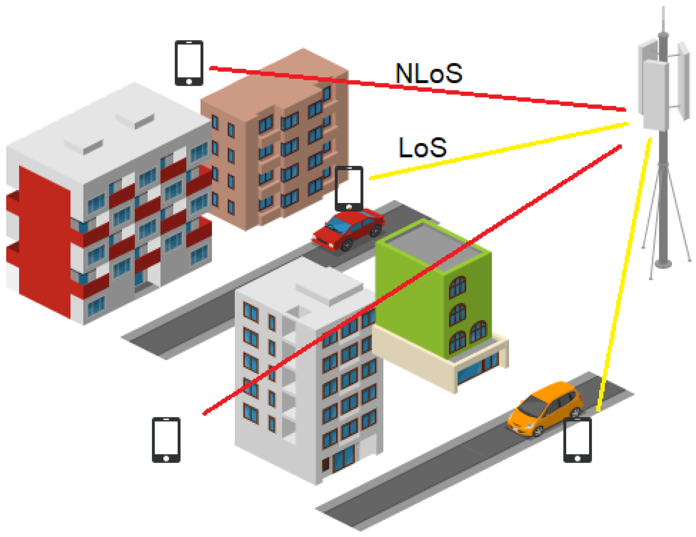
  12. Huang, C.; Molisch, A.F.; Wang, R.; Tang, P.; He, R.; Zhong, Z. Angular Information-Based NLOS/LOS Identification for Vehicle to Vehicle MIMO System. In Proceedings of the 2019 IEEE International Conference on Communications Workshops (ICC Workshops), Shanghai, China, 20–24 May 2019; pp. 1–6. [Google Scholar] [CrossRef]
  13. Yu, Y.; Liu, F.; Mao, S. Fingerprint Extraction and Classification of Wireless Channels Based on Deep Convolutional Neural Networks. Neural Process. Lett. 2018, 48, 1767–1775. [Google Scholar] [CrossRef]
  14. Zaki, A.; Métwalli, A.; Aly, M.H.; Badawi, W.K. Enhanced feature selection method based on regularization and kernel trick for 5G applications and beyond. Alex. Eng. J. 2022, 61, 11589–11600. [Google Scholar] [CrossRef]
  15. Zhang, J.; Liu, L.; Fan, Y.; Zhuang, L.; Zhou, T.; Piao, Z. Wireless Channel Propagation Scenarios Identification: A Perspective of Machine Learning. IEEE Access 2020, 8, 47797–47806. [Google Scholar] [CrossRef]
  16. Fleury, B.; Jourdan, P.; Stucki, A. High-resolution channel parameter estimation for MIMO applications using the SAGE algorithm. In Proceedings of the 2002 International Zurich Seminar on Broadband Communications Access-Transmission-Networking (Cat. No. 02TH8599), Zurich, Switzerland, 19–21 February 2002; p. 30. [Google Scholar] [CrossRef]
  17. Al-Samman, A.M.; Hindia, M.N.; Rahman, T.A. Path loss model in outdoor environment at 32 GHz for 5G system. In Proceedings of the 2016 IEEE 3rd International Symposium on Telecommunication Technologies (ISTT), Kuala Lumpur, Malaysia, 28–30 November 2016; pp. 9–13. [Google Scholar] [CrossRef]
  18. Doukas, A.; Kalivas, G. Rician K Factor Estimation for Wireless Communication Systems. In Proceedings of the 2006 International Conference on Wireless and Mobile Communications (ICWMC’06), Bucharest, Romania, 29–31 July 2006; p. 69. [Google Scholar] [CrossRef]
  19. Arslan, H.; Yucek, T. Delay spread estimation for wireless communication systems. In Proceedings of the 8th IEEE Symposium on Computers and Communications (ISCC 2003), Kemer-Antalia, Turkey, 30 June–3 July 2003; Volume 1, pp. 282–287. [Google Scholar] [CrossRef]
  20. Alshammari, A.; Albdran, S.; Ahad, A.R.; Matin, M. Impact of angular spread on massive MIMO channel estimation. In Proceedings of the 2016 19th International Conference on Computer and Information Technology (ICCIT), Dhaka, Bangladesh, 18–20 December 2016; pp. 84–87. [Google Scholar] [CrossRef]
  21. Raju, V.N.G.; Lakshmi, K.P.; Jain, V.M.; Kalidindi, A.; Padma, V. Study the Influence of Normalization/Transformation process on the Accuracy of Supervised Classification. In Proceedings of the 2020 Third International Conference on Smart Systems and Inventive Technology (ICSSIT), Tirunelveli, India, 20–22 August 2020; pp. 729–735. [Google Scholar] [CrossRef]
  22. Muthukrishnan, R.; Rohini, R. LASSO: A feature selection technique in predictive modeling for machine learning. In Proceedings of the 2016 IEEE International Conference on Advances in Computer Applications (ICACA), Coimbatore, India, 24 October 2016; pp. 84–87. [Google Scholar] [CrossRef]
  23. Soleymani, F.; Akgül, A. Improved numerical solution of multi-asset option pricing problem: A localized RBF-FD approach. Chaos Solitons Fractals 2019, 119, 298–309. [Google Scholar] [CrossRef]
  24. Taunk, K.; De, S.; Verma, S.; Swetapadma, A. A Brief Review of Nearest Neighbor Algorithm for Learning and Classification. In Proceedings of the 2019 International Conference on Intelligent Computing and Control Systems (ICCS), Madurai, India, 15–17 May 2019; pp. 1255–1260. [Google Scholar]
  25. Badawi, W.K.; Osman, Z.M.; Sharkas, M.A.; Tamazin, M. A classification technique for condensed matter phases using a combination of PCA and SVM” Progress. In Proceedings of the Electromagnetics Research Symposium (PIERS), St. Petersburg, Russia, 22–25 May 2017; pp. 326–331. [Google Scholar]
  26. Chang, C.-I. An Effective Evaluation Tool for Hyperspectral Target Detection: 3D Receiver Operating Characteristic Curve Analysis. IEEE Trans. Geosci. Remote Sens. 2020, 59, 5131–5153. [Google Scholar] [CrossRef]
Figure 1. ML concern in physical, middle, and end-user layers.
Electronics 11 03253 g001
Figure 2. LoS and NLoS scenarios.
Electronics 11 03253 g002
Figure 3. Model planning procedures: data preprocessing, data ML processing, and model evaluation.
Electronics 11 03253 g003
Figure 4. ROC curve illustration.
Electronics 11 03253 g004
Figure 5. Correlation matrices of the inter-parameter correlations of different scenarios.
Electronics 11 03253 g005aElectronics 11 03253 g005b
Figure 6. PDF of k-PCA output components.
Electronics 11 03253 g006
Figure 7. ROC and AUC scores for each scenario versus the others.
Electronics 11 03253 g007aElectronics 11 03253 g007b
Table 1. LASSO and ElasticNet feature selection decision.
FeaturesesAKFPLasAesDasDDS
Method
LASSO (Present Work)KeptKeptKeptKeptDroppedDroppedDropped
ElasticNet Ref. [14]KeptKeptKeptKeptDroppedDroppedDropped
Table 2. LASSO and ElasticNet time evaluation.
ModelRuntime (s)
LASSO (Present Work)0.33
ElasticNet (Ref. [14])0.67
Table 3. Time evaluation of each algorithm.
AlgorithmsKNNSVMk-MeansGMM
Accuracy99%99%97%98%
Fit & Predict Time (s)0.1810.1550.260.087
Publisher’s Note: MDPI stays neutral with regard to jurisdictional claims in published maps and institutional affiliations.

