Evaluating the Efficiency of Connected and Automated Buses Platooning in Mixed Traffic Environment

Abstract

Due to the battery capacity limitation of battery electric vehicles (BEVs), the importance of minimizing energy consumption has been increasing in recent years. In the mean time, for improving vehicle energy efficiency, platooning has attracted attention of several automakers. Using the connected and automated vehicles (CAVs) technology, platooning can achieve a longer driving range while preserving a closer distance from the preceding vehicle, resulting in the minimization of the aerodynamic force. However, undesired behaviors of human-driven vehicles (HVs) in the platooning group can prohibit the maximization of the energy efficiency. In this paper, we developed a speed planner based on the model predictive control (MPC) to minimize the total platooning energy consumption, and HVs were programmed to maintain a long enough distance from the preceding vehicle to avoid collision. The simulations were performed to determine how HV influences the efficiencies of the platooning group, which is composed of CAVs and HVs together, in several scenarios including the different positions and numbers of the HVs. Test results show that the CAVs planned by our approach reduces energy consumption by about 4% or more than 4% compared to that of the HVs.

1. Introduction

Eco-friendly vehicles such as battery electric vehicles (BEVs) have been promoted to counter environmental issues, but their driving range is limited due to the limitation of the battery capacity [1,2]. Therefore, since the 20th century, the development of energy saving approaches to increase energy efficiency has attracted attention of many automakers. Some researchers have developed an optimal velocity planning scheme using traffic signal phase and timing (SPAT) [3,4], efficient regenerative braking systems to recharge batteries [5], and energy-efficient cabin climate control [6,7].

In addition, many researchers have proposed platooning using vehicle to everything (V2X) connection to improve energy efficiency [8,9,10]. The vehicles in platooning drive along the same trajectory, maintaining short inter-vehicle distance. The effect of improving energy efficiency and highway capacity can be achieved by platooning. To provide consistent signal coverage, a wireless communication infrastructure is necessary for vehicular communication. Vehicles exchange information about the local traffic conditions, and this advanced technology has led to the connected and automated vehicles (CAVs) [11,12,13,14]. This advancement can be exploited to form a group of vehicles that travel together to maximize energy efficiency. A small inter vehicle distance allows the platooning group to reduce the overall air resistance. For example, refs. [15,16] show how drag coefficient influences the energy consumption according to inter-vehicle distance. Depending on the number of vehicles, the air drag coefficient of vehicles in the group can be reduced by 40% [17]. This impact reduces the total air resistance of vehicles, thereby reducing energy consumption [18,19,20].

However, previous studies have not considered mixed CAVs and human-vehicles (HVs) in a specific platooning group. Communication between vehicles is difficult in this case because the HVs are disconnected from the CAVs. That is, the driving intention of HV is not unknown to CAV by nature. Evidently, for this disconnection, reducing the total air drag of the group is extremely grueling. From this motivation, in this paper, we develop an efficient energy platooning strategy for a group in which the CAVs and HVs coexist, and demonstrate the energy consumption results according to their formations.

Reinforcement learning (RL) is one of the theories to develop an eco-platooning strategy [21]. RL has an explosion of interest in technology to control automated vehicles, but learning-based algorithms may result in fatal accidents. Although dynamic programming (DP) can be considered, it requires the entire journey trajectory to calculate the optimal trajectory [22]. Therefore, DP cannot be implemented to real-time control. Meanwhile, model predictive control (MPC) can be considered as a solution to both safety and real-time issues. To predict optimal future the behavior, MPC calculates the trajectory of the future-modified inputs [23,24,25,26].

In this study, we exploit MPC and vehicle speed preview using V2X to plan energy efficiency platooning with mixed CAVs and HVs in the group. The main objective of this study is to create an optimized path for CAVs using the expected vehicle information. CAVs in platooning aim to reduce the overall energy consumption of the group. In addition, we analyzed how HVs affect energy consumption according to the platooning formation. The main contributions of this study are as follows:

(1) We propose the CAVs platooning control algorithm using MPC. Using predicted vehicle information, CAVs optimize speed trajectory to minimize the total platooning energy consumption, and the effectiveness is confirmed through simulations under various conditions.

(2) We analyze the energy consumption with respect to platooning formation mixed with HVs. Although HVs are disconnected with CAVs, we estimate the HVs behavior to keep short distance from the preceding vehicle as much as possible to minimize air resistance.

The rest of this paper is organized as follows. In Section 2, we define the problem formulation for the case of mixed CAVs and HVs for platooning. In Section 3, we present the simulation modeling for the electric bus, and compare vehicle model from Autonomie with the control-oriented model. Autonomie [27] offers a reliable model and a small discrepancy with the test results. In Section 4, we present a platooning strategy that minimize energy consumption. In Section 5, we introduce the intelligent driving model (IDM) for HV model and estimate the behavior of a HV using a particle filter. The simulation results are discussed in Section 6 followed by the summary and conclusions in Section 7.

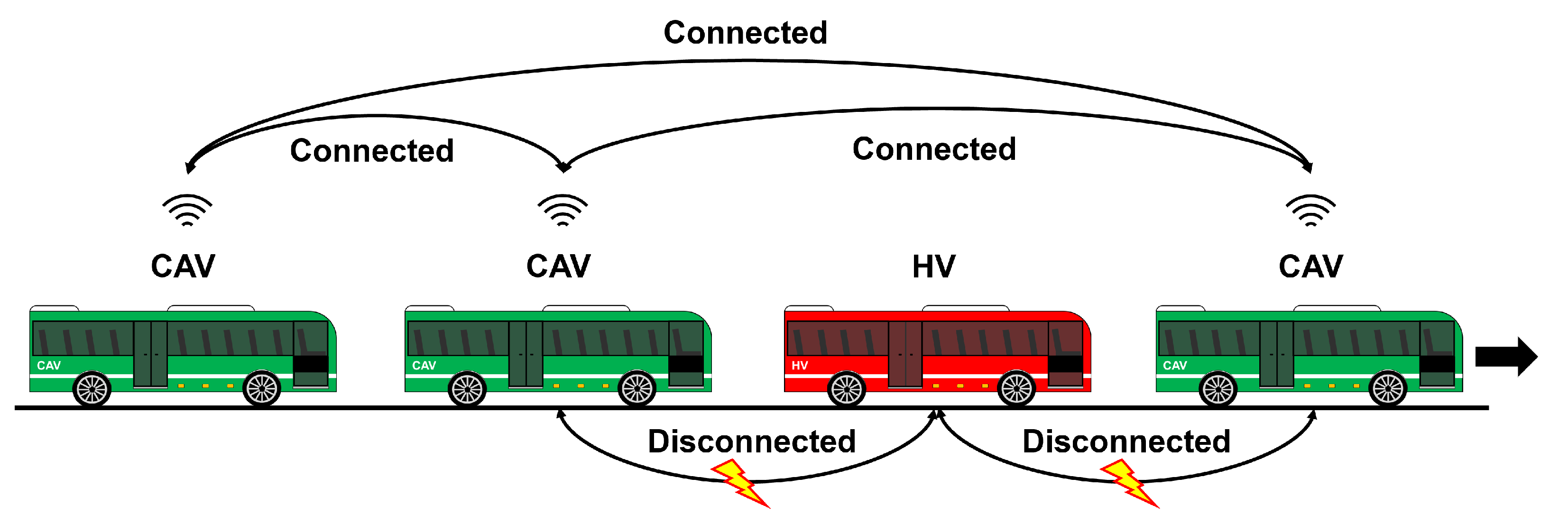
2. Problem Formulation

Figure 1 depicts an illustration of the platooning scenario. Leading vehicle is considered as a CAV in platooning for complete communication links. We assume that CAVs are connected to predecessor-leader-following (PLF) communication [28]. Owing to its complete communication links, the PLF communication topology performs better than the others, leading to the prediction of the future CAV behavior. This advantage allows us to adapt MPC to optimize path planning. Nevertheless, CAVs are connected to each other, whereas HVs are disconnected from CAVs. This implies that HVs cannot provide the predicted behavior. In this study, we assume that the HV position can be detected with noise and we propose the estimation of HVs speed using a particle filter. We used this information to maintain a short inter-vehicle distance from the preceding HV. The measurement of inter-vehicle distance is an important issue for the safety and reduction of air resistance in platooning [29].

3. System Modeling

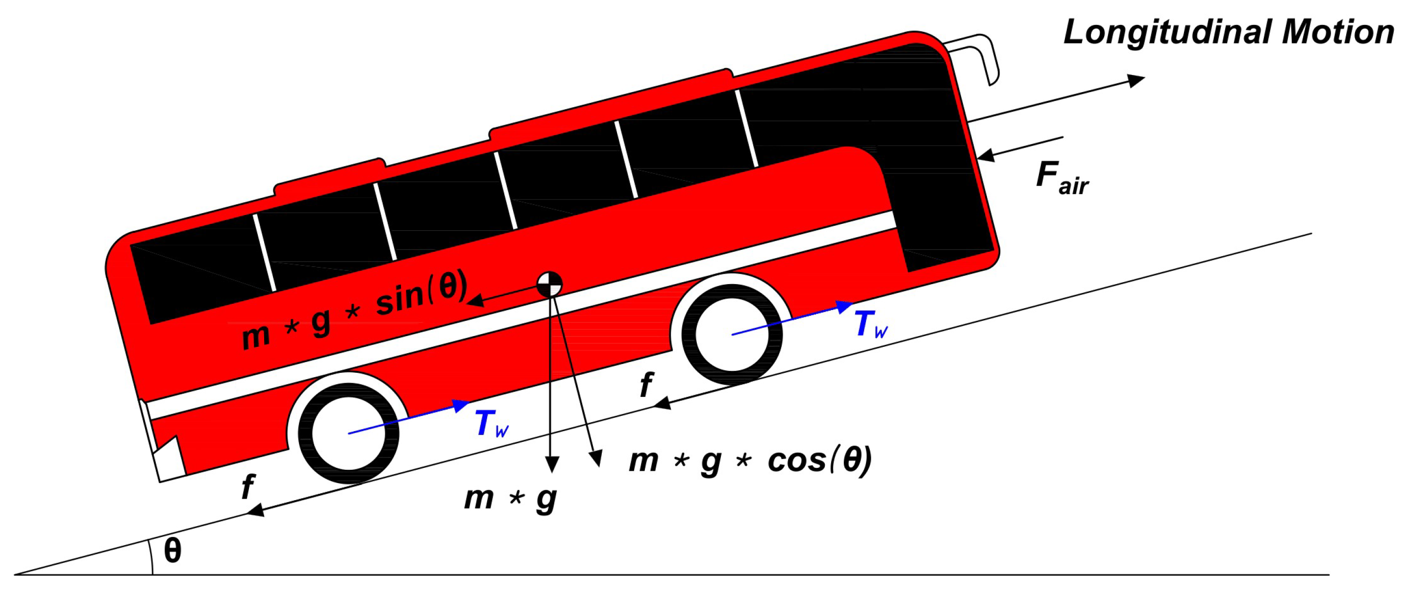
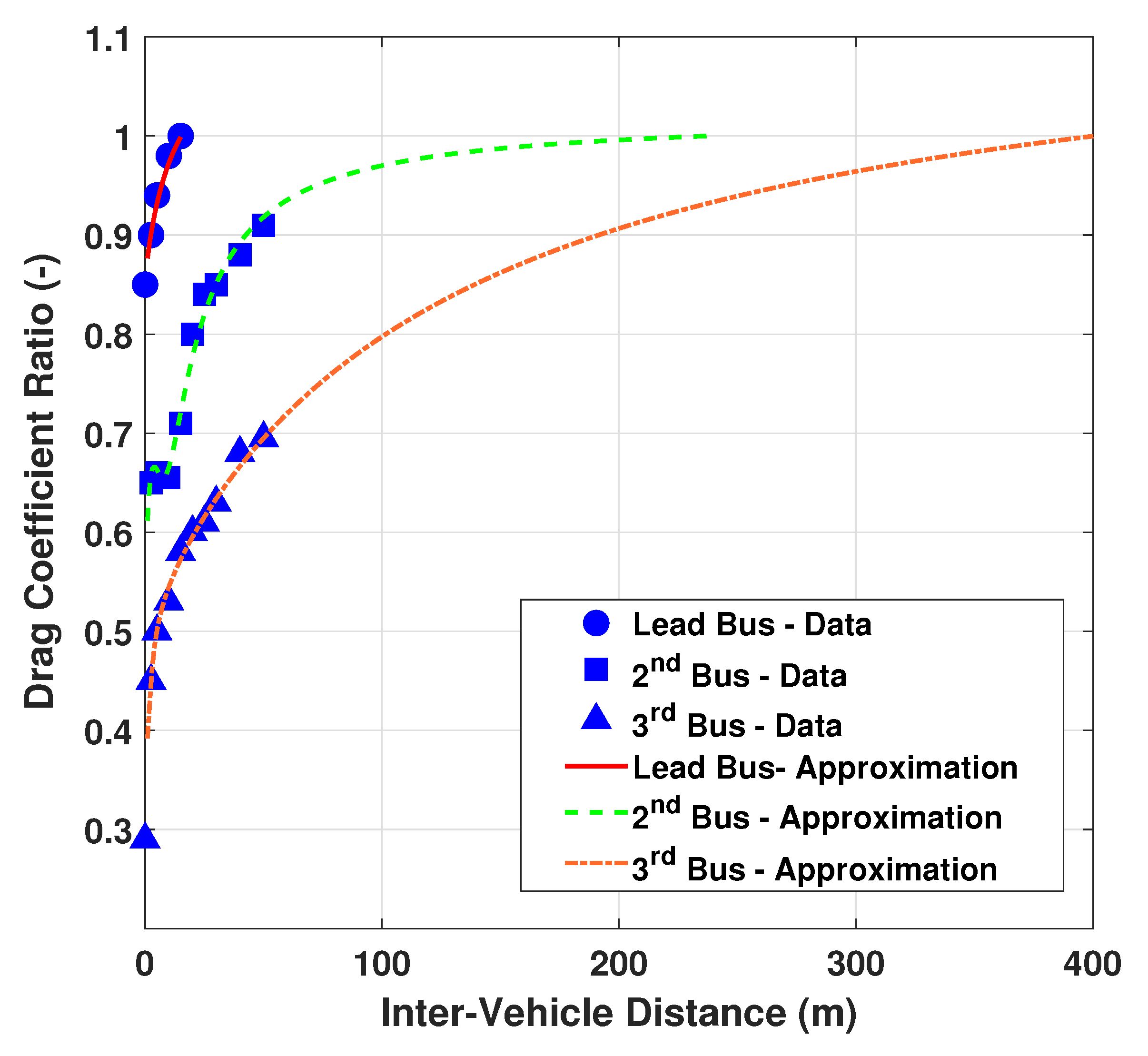
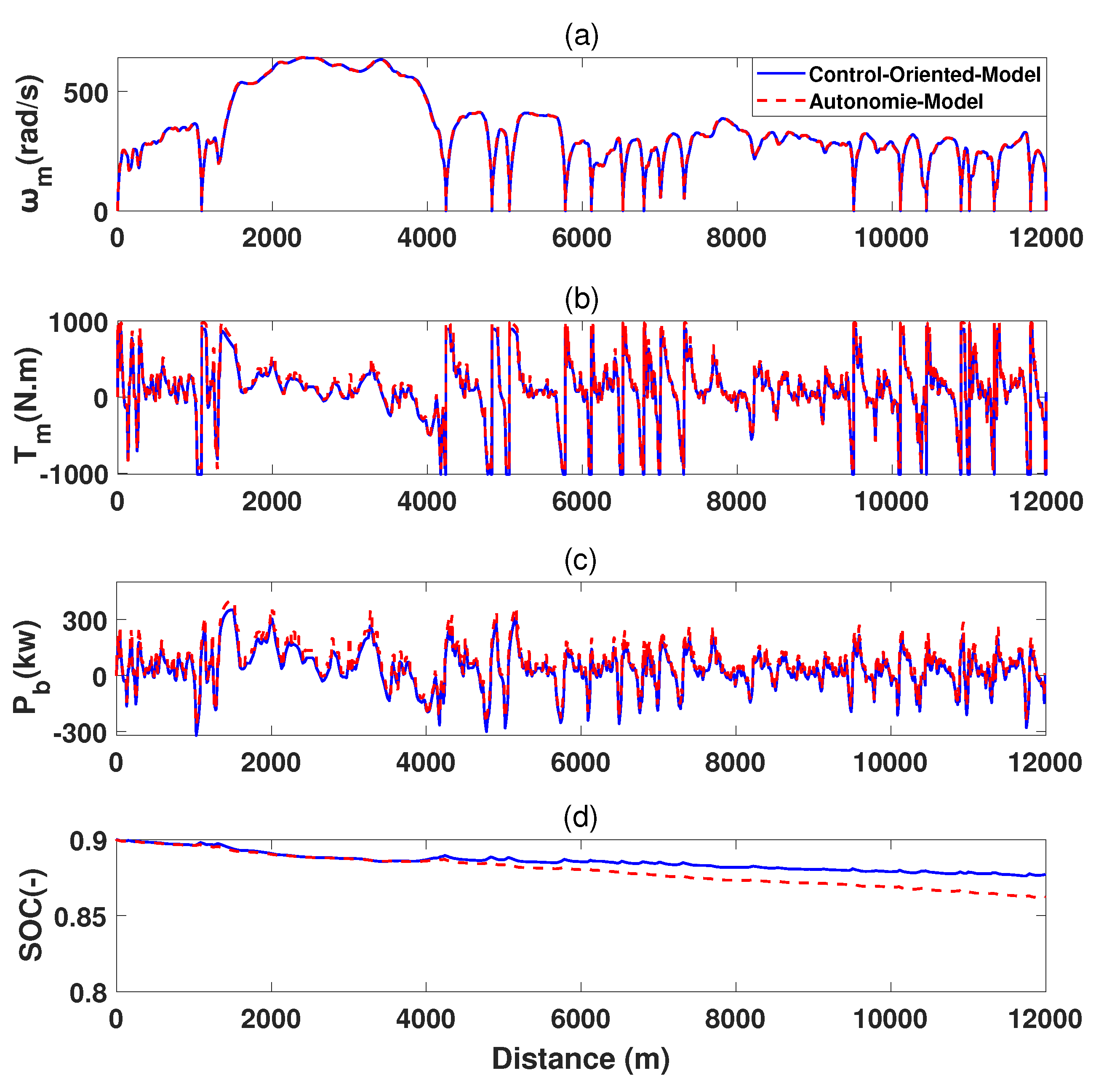
3.1. Vehicle Longitudinal Dynamics

As shown in Figure 2, in this subsection, the longitudinal dynamics of the vehicle are described. In this study, we assume that vehicles only drive in a longitudinal direction. The disturbances like cut-in and the lane-changing maneuver is not considered. The vehicle longitudinal dynamics is as follows.

$$\begin{array}{cc}\hfill \dot{s}& =v\hfill \end{array}$$

(1)

$$\begin{array}{cc}\hfill \dot{v}& =\frac{T_w}{mr}-\frac{1}{2m}\rho A{C}_d{C}_f{v}^2-g\sin \theta -fg\cos \theta \hfill \end{array}$$

(2)

where s denotes travel distance of the vehicle, v denotes the vehicle speed, $T_w$ denotes the applied input wheel torque, m denotes the vehicle mass, r denotes the wheel radius, $\rho$ denotes the air density, A is the frontal area of the vehicle, g denotes the constant as gravity, $\theta$ denotes the road slope, f is the rolling resistance coefficient, $C_d$ is the drag coefficient, and $C_f$ is the drag coefficient ratio.

The control input, i.e., motor torque $T_m$, is calculated as follows:

$$T_m\approx \frac{T_w}{i_0}$$

(3)

where $T_w$ denotes the input wheel torque and $i_0$ denotes the final reduction gear ratio.

In general, the air resistance of individual vehicles in platoons is affected by the distance between vehicles. The numerical analysis done by Zabat et al. [30] measured aerodynamic drag coefficients of light-duty vehicles (LDVs) in the wind tunnel. The results show that shorter vehicle spaces in platoons present a reduced average drag coefficient. The average drag reduction showed up to 55% for five-vehicle platoon at inter-vehicle distance 5 m [31]. Through the drag coefficient ratio $C_f$ multiplied by aerodynamic force, the control-oriented model can be more accurate to find optimal control action. We refer Hussein et al. [32] which proposes fitting drag coefficient ratio, using rational polynomial function based on experiment measurement, and $C_f$ is defined as follows:

$$C_f=\left\{\begin{array}{cc}\frac{a_n{d}_{inter}^n+a_{n-1}{d}_{inter}^{n-1}+\dots +a_1{d}_{inter}^1+a_0}{b_n{d}_{inter}^n+b_{n-1}{d}_{inter}^{n-1}+\dots +b_1{d}_{inter}^1+b_0},\hfill & 0<G\le G_0\hfill \\ \\ 1,G\ge G_0\hfill \end{array}\right.$$

(4)

Here $C_f$ is the drag coefficient ratio between the ego car and the preceding car, $d_{inter}$ is the distance gap, $a_n$ and $b_n$ are calibrated constants, and n denotes the number of vehicles in the convoy.

If a single vehicle in the platoon exceeds the critical inter-vehicle distance $G_0$, the vehicle is not susceptible to the drag coefficient ratio (i.e., $C_f=1$). Therefore, the inter-vehicle distance of a single vehicle must be less than $G_0$ in order to take advantage of the drag coefficient ratio’s benefit. The ego vehicle’s $C_f$ is calculated using $d_{inter}$ between the ego and its preceding vehicle at time k. $d_{inter}$ at time k can be calculated as follows:

$$d_{inter}=d_p-d_e$$

(5)

where $d_p$ is the preceding car’s and $d_e$ is the ego car’s inter-vehicle distance.

As shown in Figure 3, actual and approximated drag coefficient ratio $C_f$ data set for three-buses in platoons is depicted. The drag coefficient ratio of individual vehicles in platoon increases exponentially until inter-vehicle distance approaches critical point $G_0$. Although $C_f$ can be minimized as $d_{inter}$ approaches zero, we specify the minimum $d_{inter}$ value to keep the safety. In addition, it is assumed that the third car in the platoon’s drag reduction is the same from the perspective of the vehicle behind it. This model was developed by [32] and was obtained using empirical dataset [33]. The parameters data empirically fitted for $C_f$ are listed in

Table 1. Parameters of the drag coefficients ratio for individual bus platoons [32].

Parameters	Bus Platoon
	Two Buses		Three Buses
	Lead	Trail	Lead	Middle	Trail
$a_3$	$-1.5175\times {10}^{-4}$	$-7.2951\times {10}^{-4}$	$-1.5175\times {10}^{-4}$	4.7945$\times {10}^3$	9.3348$\times {10}^{-2}$
$a_2$	1.3115$\times {10}^{-1}$	4.4369$\times {10}^{-1}$	1.3115$\times {10}^{-1}$	$-4.0404\times {10}^4$	5.1656
$a_1$	1.5396	6.1509	1.5369	3.5213$\times {10}^5$	−3.9662
$a_0$	3.4243$\times {10}^{-1}$	1.1174$\times$10	3.4243$\times {10}^{-1}$	1.0311$\times {10}^6$	6.7697
$b_3$	$-8.9422\times {10}^{-5}$	$-8.5027\times {10}^{-4}$	$-8.9422\times {10}^{-5}$	4.6933$\times {10}^3$	8.1124$\times {10}^{-2}$
$b_2$	1.1463$\times {10}^{-1}$	4.6002$\times {10}^{-1}$	1.1463$\times {10}^{-1}$	$-1.6202\times {10}^4$	1.0062$\times 10$
$b_1$	1.7730	$1.2569\times 10$	1.7730	2.9853$\times {10}^5$	−4.2684
$b_0$	4.0877$\times {10}^{-1}$	1.9639$\times$10	4.0877$\times {10}^{-1}$	1.9158$\times {10}^6$	1.4692$\times 10$
$G_0$	-	3.0815$\times {10}^2$	-	2.4082$\times {10}^2$	4.0045$\times {10}^2$

.

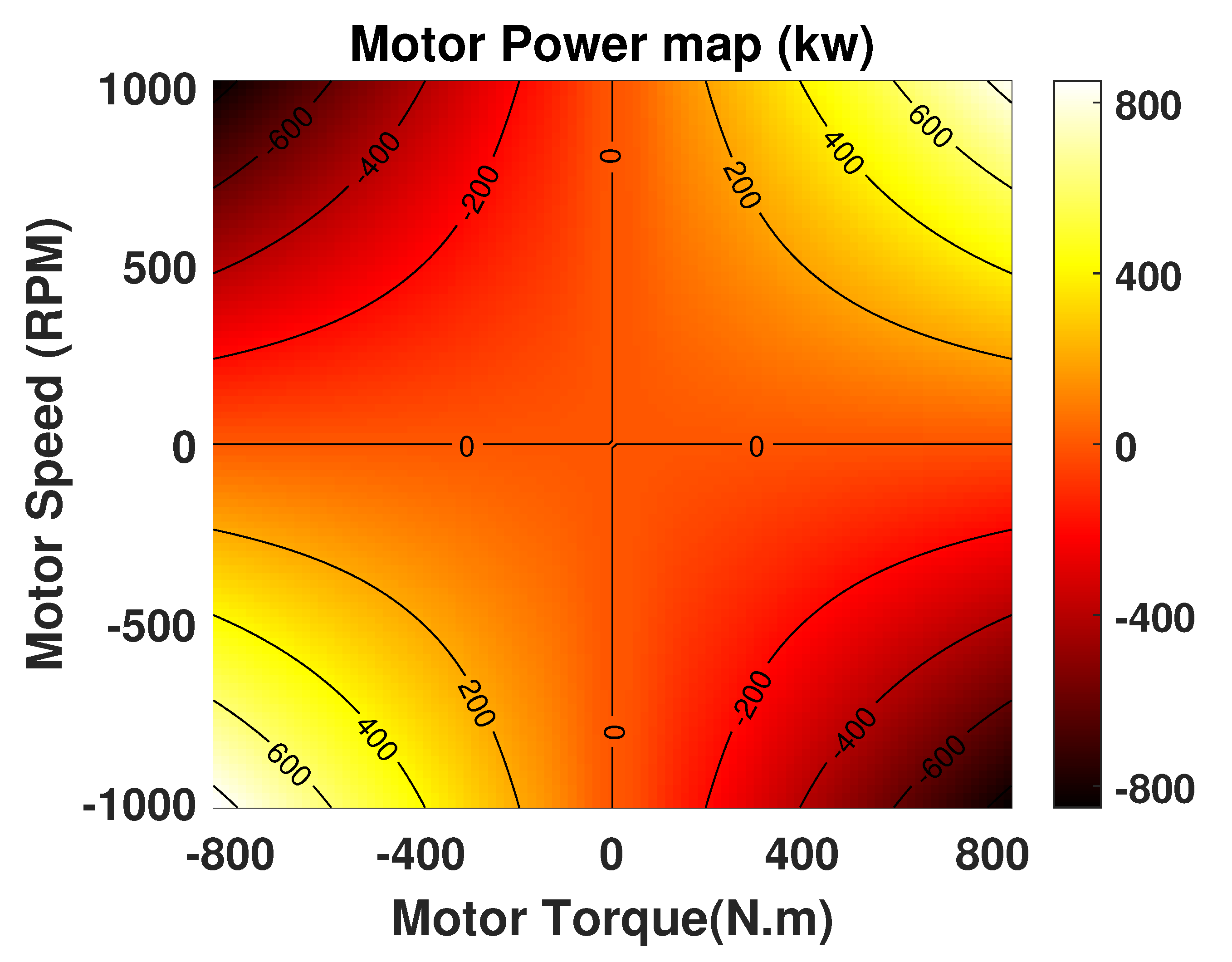
3.2. Battery Dynamics

In this subsection, we introduce the battery dynamics to calculate required energy to generate the vehicle traction force. The battery state of charge ($SOC$) is as follows:

$$SOC\left(t\right)=SOC\left(t_0\right)-\frac{{\int }_{t_0}^t{I}_b\left(t\right)dt}{C}$$

(6)

where $I_b$ denotes the battery current, and C is the battery maximum capacity.

The $SOC$ is estimated based on battery current condition. The battery current $I_b$ is calculated as follows:

$$I_b\left(t\right)=\frac{P_b\left(t\right)}{V\left(t\right)}$$

(7)

where $P_b$ is the battery power, and V denotes the battery voltage. The battery is discharged when $P_b$ is positive, and charging when $P_b$ is negative. The $P_b$ expressed described as follows:

$$P_b=\left\{\begin{array}{cc}{P}_m{e}_b,\hfill & P_m<0\hfill \\ \frac{P_m}{e_b},\hfill & P_m\ge 0\hfill \end{array}\right.$$

(8)

where $P_m$ is the motor power, which is positive when motor power is used to produce traction force, and $e_b$ is the battery efficiency. To obtain $P_m$, we used a look-up table indexed by the motor speed and torque (see Figure 4).

As shown in Figure 5, the control-oriented and Autonomie models are compared. The simulation results [27] show the accuracy of the vehicle model provided by Autonomie. In this study, the simulation was implemented by using the UDDS velocity profile and the parameters of the vehicle model are listed in

Table 2. Electric-bus parameter values offered from AMBER [34].

Description	Symbol	Value
Mass of the vehicle	m	19,717 [kg]
Wheel radius	r	0.4655 [m]
Ratio for single reduction gear	$i_0$	11.76 [-]
Frontal area	$A_f$	7.33 [m${}^2$]
Coefficient of rolling resistance	f	0.00863 [-]
Drag coefficient	$C_d$	0.65 [-]
Battery voltage	V	[3.5 4.2] [V]
Battery efficiency	$e_b$	0.9 [-]
Maximum capacity of battery	$C_b$	33.1 [Ah]
SOC range	$SOC$	[0 1] [-]
Gravity	g	9.81 [m/s${}^2$]
Air density	$\rho$	1.1985 [kg/m${}^3$]

. The discrepancy in the SOC between the control oriented model and the Autonomie is 1.75%. Through this simulation, we developed a reliable vehicle model for electric buses.

4. Nonlinear Programming Problem

The optimal control was designed to minimize the energy consumption. The key idea of our approach is to maximize regenerative braking and minimize air resistance by considering highway road information. We propose the design of the cost function and control constraints for the prediction and control horizon N:

$$\begin{array}{cc}\hfill & \underset{u\in U}{min}\sum _{k=0}^{N-1}{W}_1{P}_b\left(k\right|i)+W_2{C}_f\left(k\right|i)\hfill \\ \hfill & \mathrm{subject}\mathrm{to}\hfill \end{array}$$

(9a)

$$\begin{array}{cc}\hfill & T_m^{\min }<u\left(k\right|i)<T_m^{\max }\hfill \end{array}$$

(9b)

$$\begin{array}{cc}\hfill & d_{inter}^{\min }<d_{inter}(k+1|i)<d_{inter}^{\max }\hfill \end{array}$$

(9c)

$$\begin{array}{cc}\hfill & v^{\min }(k+1|i)<v(k+1|i)<\eta ·{\widehat{v}}^p(k+1|i)\hfill \\ \hfill & k=0,1,2\cdots ,N-1,\hfill \end{array}$$

(9d)

where $W_1,W_2$ is the weight factor, [$T_m^{min}$, $T_m^{max}$] is the restricted rage of control input, and [$d_{inter}^{min}$, $d_{inter}^{max}$] is the predefined range of the inter-vehicle distance while avoiding vehicle collisions and reducing the drag coefficient. $\eta$ is a safety variable, ${\widehat{v}}^p$ denotes preceding vehicle velocity and $i+k$ is obtained at time instant i. We tuned $W_1,W_2$ factors according to road information to maximize energy efficiency.

5. Car-Following Model and Velocity Estimation

In this section, we introduce an intelligent driver model (IDM) to model collision-free car following motion. Since the communication between HVs and CAVs is not available, the behavior of HV is highly uncertain. For this reason, the CAV following the HV employs the IDM because using the MPC with predicted information is not available. Also, a particle filter is used to estimate the HV’s velocity using the sensor measurements [35,36].

5.1. Intelligent Driving Model

The IDM model can adjust the desired safety time gap and the longitudinal velocity [37]. The IDM model is given by

$$\dot{v}\left(t\right)=a\left[1-{\left(\frac{v\left(t\right)}{v_0}\right)}^{\delta }-{\left(\frac{s^{*}(v,\Delta v)}{s\left(t\right)}\right)}^2\right]$$

(10)

where a denotes the maximum acceleration, $v_0$ denotes the preferred velocity, and $s^{*}(v,\Delta v)$ denotes the desired gap. The desired gap $s^{*}(v,\Delta v)$ is given by

$$s^{*}\left(v,\Delta v\right)=s_0+s_1\sqrt{\frac{v}{v_0}}+T_{h}v+\frac{v\Delta v}{2\sqrt{ab}}$$

(11)

where $s_0$ and $s_1$ are the minimum gap when following other vehicles, $T_h$ denotes time headway, and b denotes the characterized deceleration.

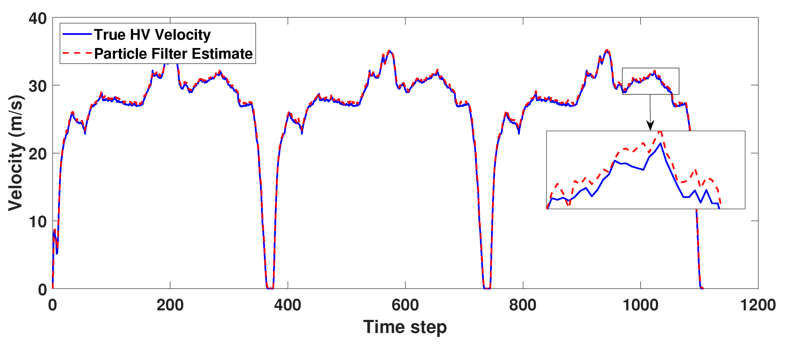
5.2. Particle Filter-Based Velocity Estimation

In this subsection, we propose a method of estimating HV’s velocity using particle filter (a.k.a. sequential Monte Carlo) in order to keep the safe-distance while following. Since HV drives stochastically at every moment, we should estimate HV’s velocity through a probability-based particle filter. The basic principle of the particle filter is well described in [38].

It is assumed that the preceding HV’s position is measured continuously and this position information is used to estimate the HV’s state variable $x_{k+1}$. The current state $x_k$ is calculated by the measurement during the sampling time. The distribution of particles should be conducted because the future HV’s behavior is predicted based on probability. For this reason, we randomly scattered particles to find the behavior of HV that most likely to happen. The distribution is calculated as follows.

$$\begin{array}{cc}\hfill x_{k+1,i}& =f_k(x_{k,i},w_k)i=1,\cdots ,N\hfill \end{array}$$

(12)

where k indicates the time instance, $x_k$ is the state variable, $w_k$ is the process noise, $T_s$ is the sampling time, $z_k$ is the measurement noise, i is the index for the particle, and N is the number of particles generated via trial-and-error. We randomly generate N particles $x_{k,i}$ at time k. In this process, white noise $w_k$ that is randomly generated is considered to prevent the case that particles are distributed on the point which is much far from the actual data.

Subsequently, we weight the particles based on relative likelihood to approximate actual velocity. The relative likelihood $q_{k,i}\left(x_{k,i}\right)$ is assumed to be followed the Gaussian distribution:

$$\begin{array}{c}\hfill q_{k,i}\left(x_{k,i}\right)=\frac{1}{{\left(2\pi R\right)}^{1/2}}exp\left(\frac{-{(x_k^{*}-x_{k,i})}^2}{2R}\right)\end{array}$$

(13)

where $x_k^{*}$ is the estimated state variable at time instance k, and R is the variance.

We define a new distribution of cumulative probability function(CDF) for the resampling step. The CDF can prevent being biased by considering the only one points that lots particles are gathered when the resampling happens. The normalized relative likelihood can be expressed as follows:

$$q_i=\frac{q_i}{{\sum }_{j=1}^N{q}_j}$$

(14)

The resampling stage was conducted $q_i$ into the accumulated distribution. Based on the accumulated distribution, sum of all the normalized relative likelihood is equal to one. We randomly pick particles given weight and average them for estimation. The approximated mean of particles is given by

$$E\left(x_{k+1}\right)\approx \frac{1}{N}\sum _{i=1}^N{x}_{k,i}$$

(15)

where $E\left(x_k\right)$ denotes the expected value.

The particle $x_{k,i}$ is randomly selected in the accumulated distribution domain $q_i$ for resampling. Subsequently, the sum of the resampled particles $x_{k,i}$ is divided by the number of particles to calculate the expectation value. We set $x_k$ as HV’s velocity to keep safty distance.

As shown in Figure 6, the estimation of HV speed is depicted when it is driven based on the adapted US06 speed profile. We assumed that the HV position and state are the HV velocities. Although there are some differences between the actual and estimated data, the estimation tracks the intended acceleration and deceleration of human vehicles. Using the estimated value, the vehicle behind the HV was followed by using the IDM model.

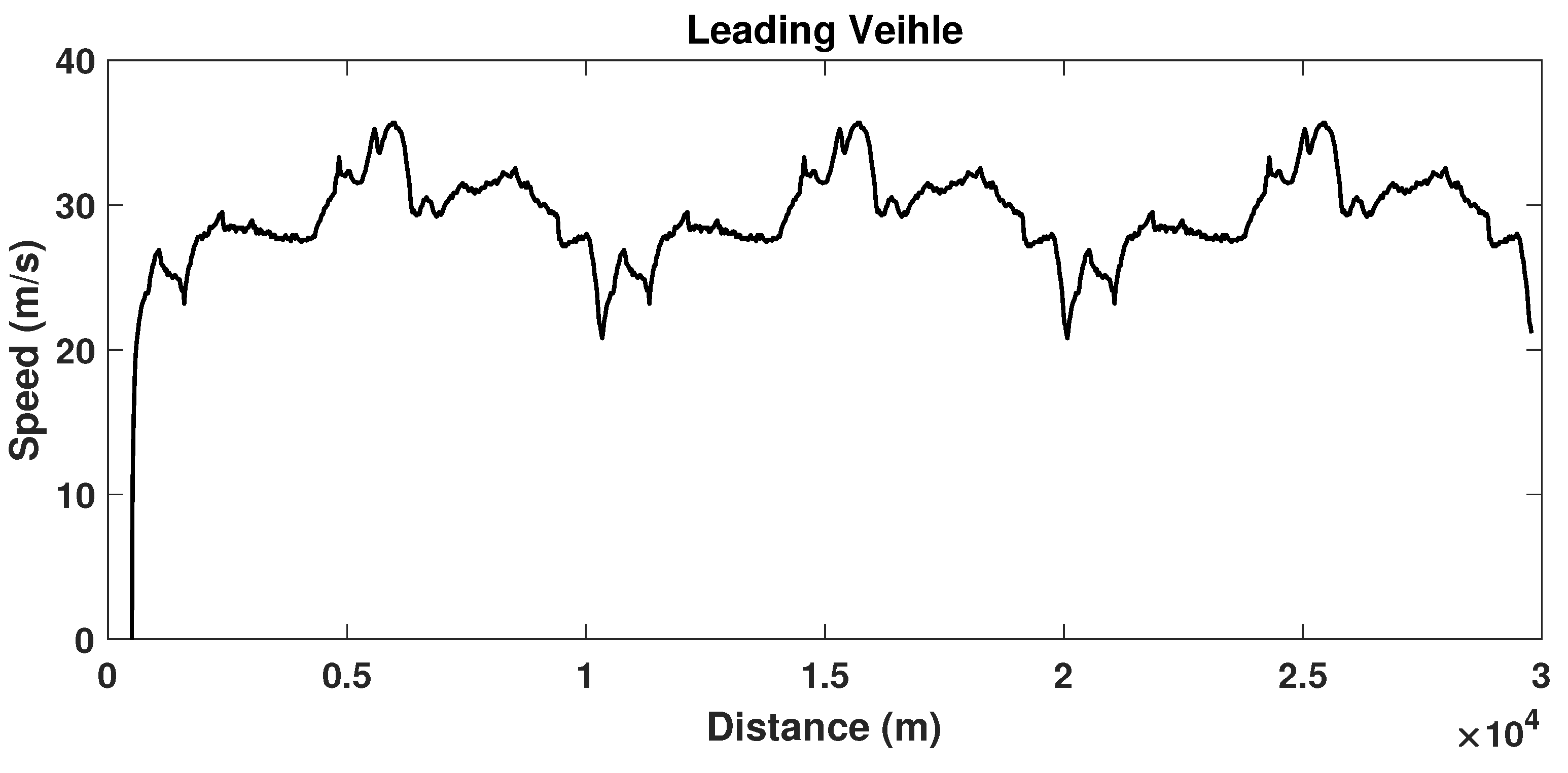
6. Simulation and Results

In this section, we evaluate developed CAV speed planner in various scenarios in terms of the energy efficiency according to the HVs position and the number of HVs. We assumed that all the leading vehicles in the scenario drive with a modified US06 speed profile in highway. The total travel distance for the leading vehicle is 29.78 km, and speed profile of the leading vehicle is shown in Figure A3. In addition, road slope information was obtained from Google Earth [39] (see Figure A1). The following vehicles travel until the leading vehicle stops. The simulation is performed in Windows 10 operating system with Intel(R) Core(TM) i5-9500, 16GB RAM memory. The MPC problem is solved by MATLAB function $fmincon\left(\right)$.

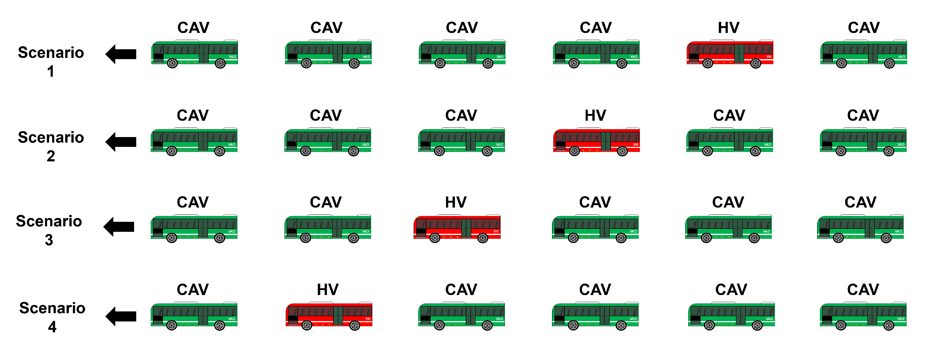
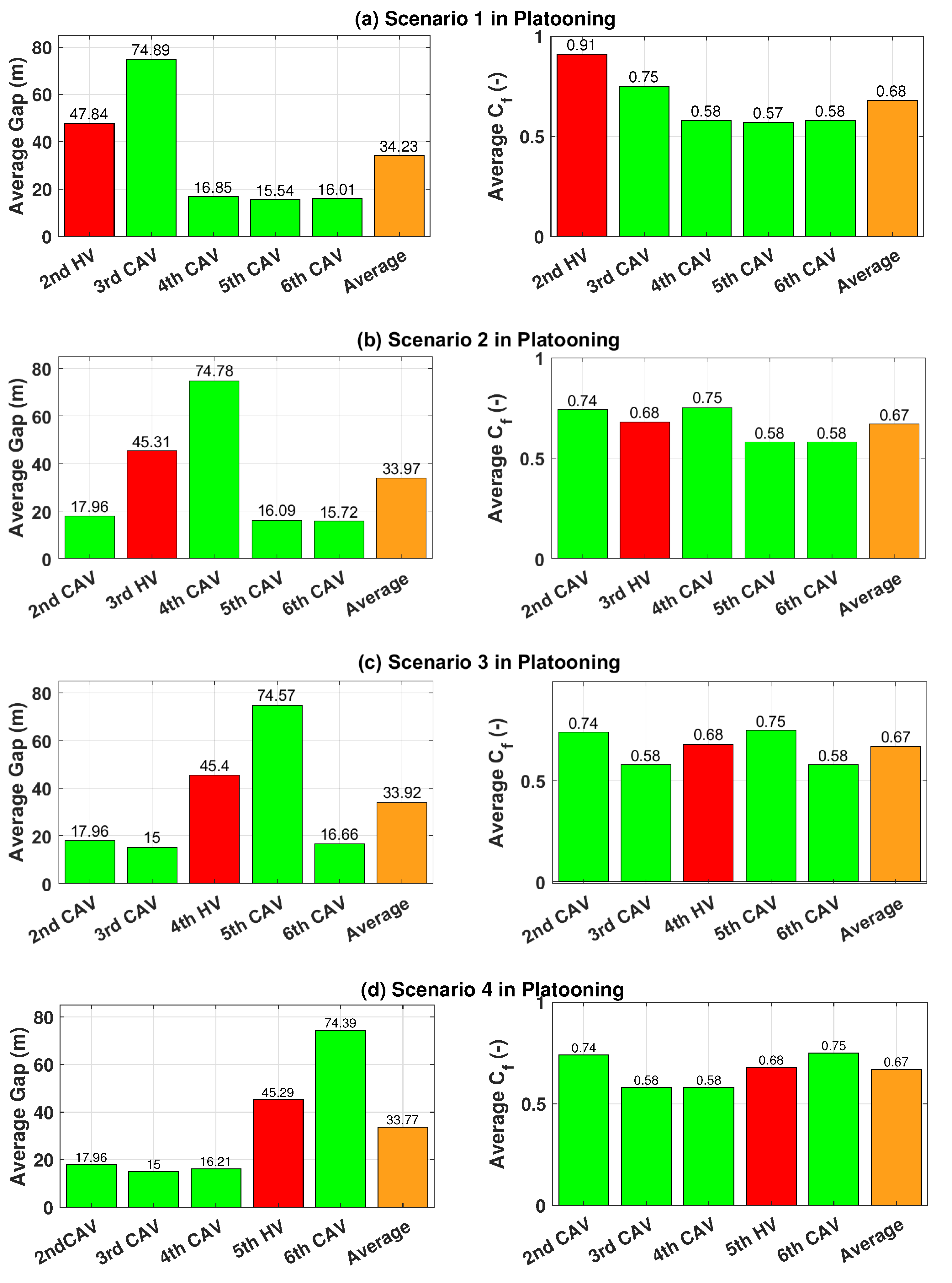
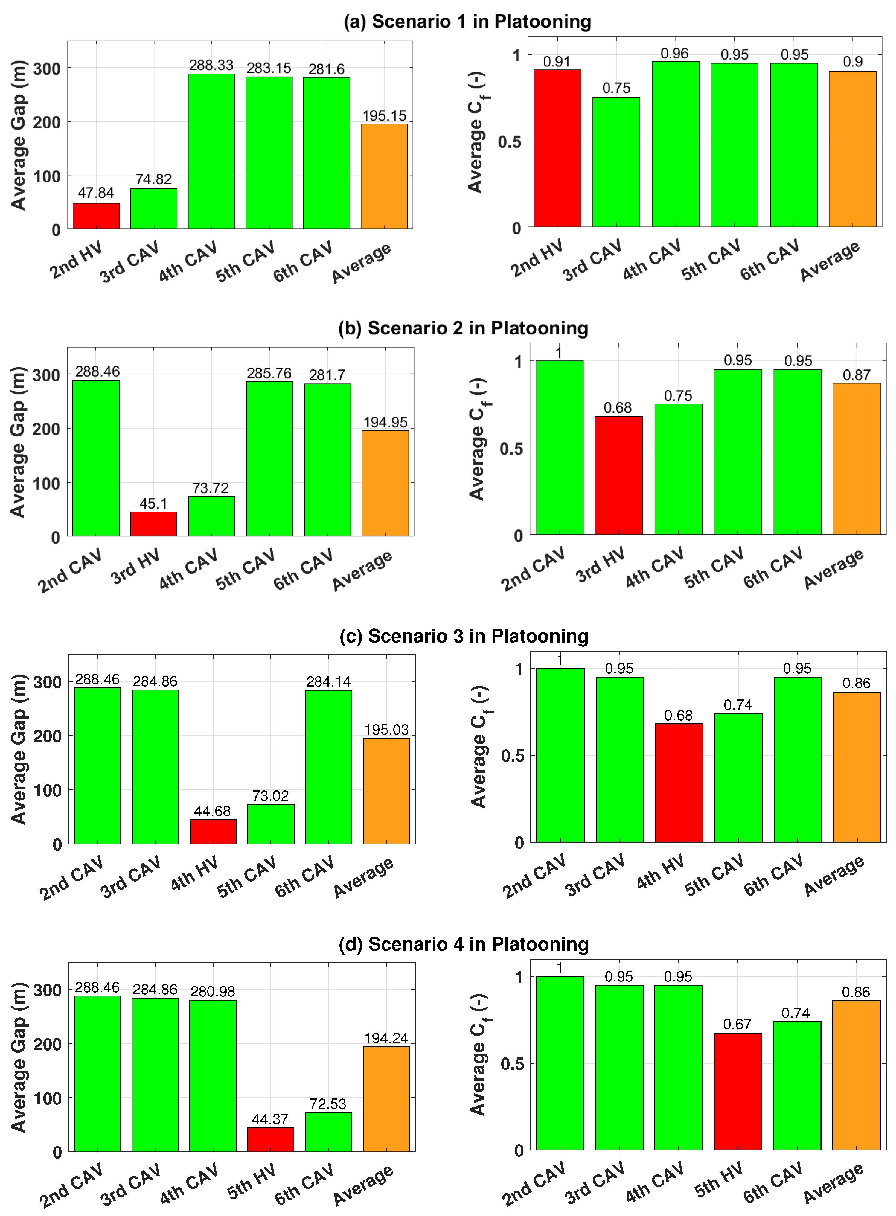
6.1. Case 1: Energy Efficiencies Depending on the Locations of HV on the Flat Road

In this subsection, four scenarios were considered, as shown in Figure 7 in which the leading CAV is assumed to drive with deformed US06 speed profile on the flat road, so the total travel distance for the leading vehicle was 29.78 km. Scenarios 1, 2, 3, and 4 are illustrated in which the HV is placed differently. Figure 8 shows the average gap and the reduced drag coefficient factor $C_f$ between the preceding and following vehicles for each scenario. The red, green, and orange bars indicate the HV, CAV, and average values, respectively.

As discussed in

Table 3. Battery SOC consumption for four scenarios in Case 1.

Scenario	1st Bus SOC (%)	2st Bus SOC (%)	3st Bus SOC (%)	4st Bus SOC (%)	5st Bus SOC (%)	6st Bus SOC (%)	Average SOC Consumption (%)
Scenario 1	22.97	22.07	20.98	18.21	17.97	17.99	20.03
Scenario 2	22.97	19.92	20.13	20.6	18.02	17.96	19.80
Scenario 3	22.97	19.32	18.15	20.15	20.68	17.99	19.84
Scenario 4	22.97	19.12	18.15	18.08	20.01	20.47	19.98

, where the aero drag coefficient decreases if the more vehicles travel in front even if the inter-distance between vehicles are same, the HV in the scenario 1 consumed more average SOC than other scenario. It is observed that the position of vehicle strongly influences on the energy consumption. Although HVs drive with similar inter-vehicle distance, drag coefficient is applied differently depending on the position (see Figure 3). As shown in Figure 8, the HV in the scenario 1 has the most biggest drag coefficient 0.91 which consumes the most battery energy.

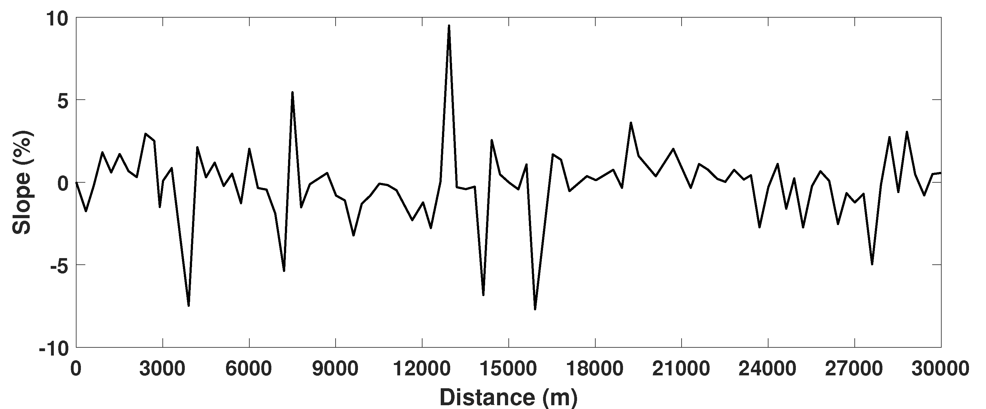
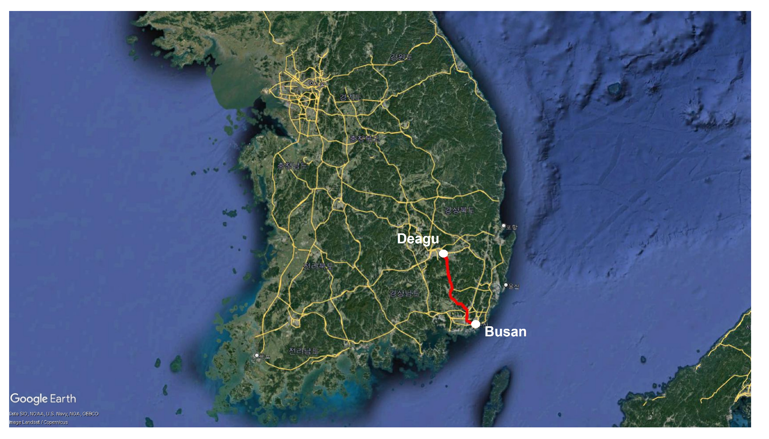
6.2. Case 2: Energy Efficiencies Depending on the Locations of HV on the Sloped Road

In this subsection, we analyze the energy efficiencies for each scenario on the sloped road (see Figure 7). Test results of each scenario’s SOC consumptions are described in

Table 4. Battery SOC consumption for four scenarios in Case 2.

Scenario	1st Bus SOC (%)	2st Bus SOC (%)	3st Bus SOC (%)	1st Bus SOC (%)	5st Bus SOC (%)	6st Bus SOC (%)	Average SOC Consumption (%)
Scenario 1	23.33	22.55	20.98	19.96	19.79	19.99	21.17
Scenario 2	23.33	20.21	20.81	21.20	19.78	20.01	20.99
Scenario 3	23.33	20.21	19.80	20.65	21.03	19.93	20.93
Scenario 4	23.33	20.21	19.80	19.78	20.71	21.16	20.94

. The SOC of CAVs following HV is higher than other vehicles. This results are caused by (9), where the vehicles use the regenerative braking function as much as possible, which is more effective than reducing drag coefficient on sloped road. In the Figure 9, CAV that located right behind of human vehicle has shorter inter-vehicle distance from the preceding car compared to other CAVs in every scenarios which have high drag coefficient. However, the SOC of CAVs which drive with long inter-vehicle distance was lower than others even though they have bigger air drag coefficients. To sum up, we can conclude that energy recovering by the regenerative braking is more effective than the reducing aero drag coefficient.

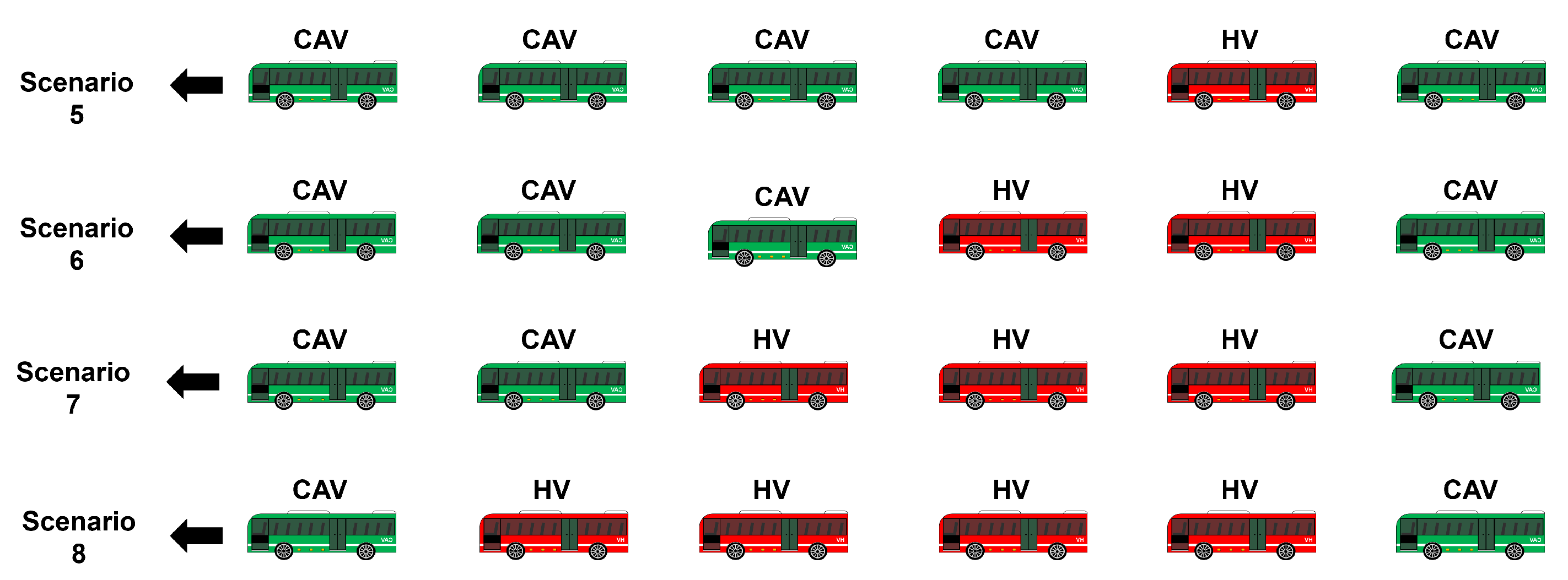
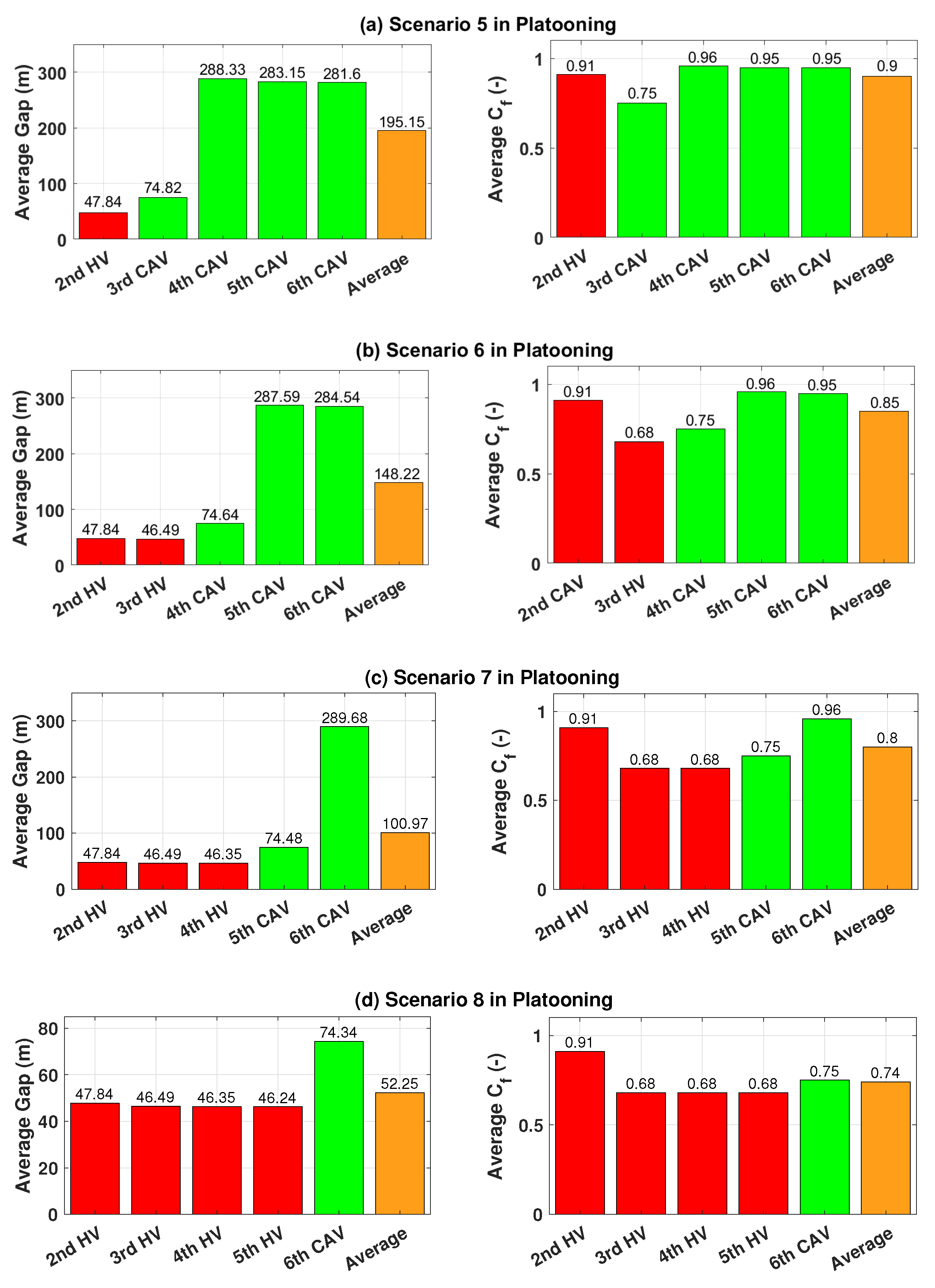
6.3. Case 3: Energy Efficiencies Depending on the Number of Multiple HVs on a Flat Road

In this section, scenarios 5, 6, 7 and 8 are considered as shown in Figure 10. Each scenario has the different number of the HV and results show how that influenced to the platooning group. As shown on the

Table 5. Battery SOC consumption for four scenarios in Case 3.

Scenario	1st Bus SOC (%)	2st Bus SOC (%)	3st Bus SOC (%)	4st Bus SOC (%)	5st Bus SOC (%)	6st Bus SOC (%)	Average SOC Consumption (%)
Scenario 5	22.97	22.07	20.98	18.21	17.97	17.99	20.03
Scenario 6	22.97	22.07	20.47	22.06	17.99	17.90	20.58
Scenario 7	22.97	22.07	20.47	20.46	20.97	18.15	20.85
Scenario 8	22.97	22.07	20.47	20.46	20.44	20.98	21.23

, the average SOC consumption results show that as the number of the HV increases, the average energy consumption tends to increase. The scenario 8 with the most number of HVs consumed an average SOC 21.23%, whereas 20.03% average SOC is consumed in Scenario 5 which has the fewest number of HVs. As shown in Figure 11, CAVs have lower drag than HVs because CAVs can maintain shorter inter-vehicle distance. The result of scenario 8 shows that scenario 8 has a higher average inter-vehicle distance than scenario 7, which leads to higher air resistance. Overall, more CAVs deployed in platoon can save energy consumption.

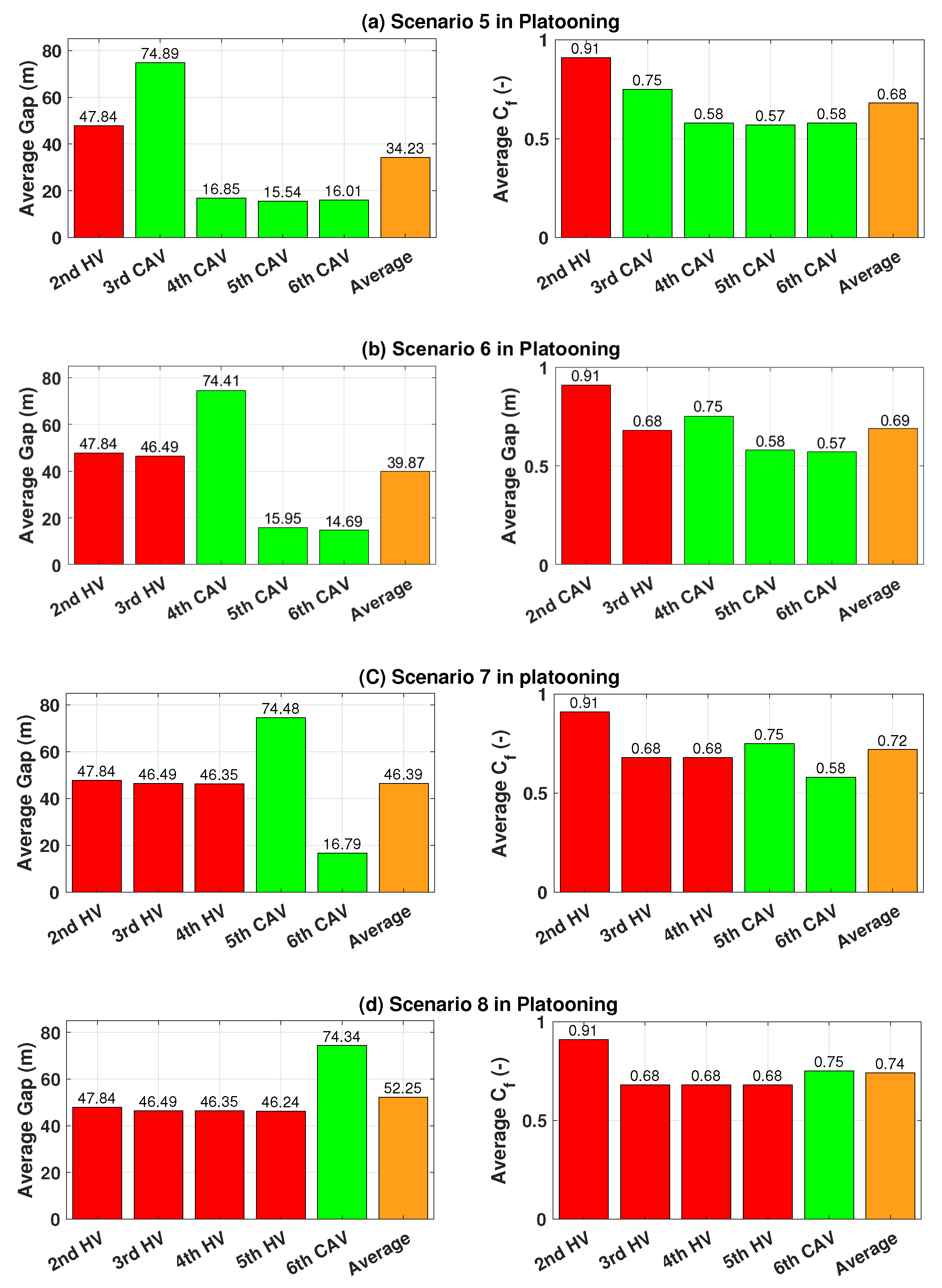
6.4. Case 4: Energy Efficiencies Depending on the Number of Multiple HVs on the Sloped Road

In this subsection, we analyze the energy efficiencies for each scenario on the sloped road (see Figure 10). Each scenario has the different number of the HV and test results show how the number of HVs between CAVs influence the energy efficiency of the vehicle group. As the number of HVs increased, the average SOC consumption also increases as depicted in

Table 6. Battery SOC consumption for four scenarios in Case 4.

Scenario	1st Bus SOC (%)	2st Bus SOC (%)	3st Bus SOC (%)	4st Bus SOC (%)	5st Bus SOC (%)	6st Bus SOC (%)	Average SOC Consumption (%)
Scenario 5	23.33	22.55	20.98	19.96	19.79	19.99	21.1
Scenario 6	23.33	22.55	21.05	21.58	19.89	19.85	21.32
Scenario 7	23.33	22.55	21.05	21.01	21.51	19.93	21.56
Scenario 8	23.33	22.55	21.05	21.01	20.99	21.57	21.75

. This is because more CAVs in platoon can save energy consumption while exploiting regenerative brake. Although the average gap and $C_f$ in scenario 5 were higher than other scenarios, they consumed lesser energy than other scenarios as shown in Figure 12. This implies that exploiting regenerative brake is more effective than reducing the air resistance on the sloped road from the perspective of saving energy.

7. Conclusions

In this paper, we propose the energy-efficient control framework for CAV in platoon and evaluate its effectiveness in mixed traffic environment. Especially, using the connectivities, the vehicles future behaviors are exploited when optimizing the velocity profiles of multiple CAVs.

The two main distinctions of this study compared to existing studies are as follows. First, the MPC-based controller for CAVs performed better than that for HVs in terms of energy efficiency. Second, we propose estimating HV’s velocity through a probability-based particle filter. The CAVs use estimated HV’s velocity to keep the safety distance while HV drives stochastically at every moment. An evaluation is performed to verify our approach under various platooning scenarios. The 5th CAV saved energy consumption by up to 4.1% compared to HV in scenario 5. In addition, as the number of HVs in a group increases, the average battery SOC consumption decrease. The average battery SOC consumption value differed by up to 1.2% depending on the number of HVs in the convoy. However, the average battery SOC consumption according to the position of the HV does not have a meaningful relationship. This is because our predefined HV travels with a reasonable inter-vehicle distance from the preceding vehicle, which can reduce energy consumption. Our approach shows that CAV only use HV’s estimated information to keep a safety distance.

In future studies, we will model the human-drivers with different driving characteristics, then we will perform hardware-in-loop (HIL) test to verify the applicability of our approach in the mixed-traffic environment in real-time.

References

1. Tran, M.-K.; Bhatti, A.; Vrolyk, R.; Wong, D.; Panchal, S.; Fowler, M.; Fraser, R. A review of range extenders in battery electric vehicles: Current Progress and Future Perspectives. World Electr. Veh. J. 2021, 12, 54. [Google Scholar] [CrossRef]
2. Lain, M.J.; Kendrick, E. Understanding the limitations of lithium ion batteries at high rates. J. Power Sources 2021, 493, 229690. [Google Scholar] [CrossRef]
3. Mahler, G.; Vahidi, A. An optimal velocity-planning scheme for vehicle energy efficiency through probabilistic prediction of traffic-signal timing. IEEE Trans. Intell. Transp. Syst. 2014, 15, 2516–2523. [Google Scholar] [CrossRef]
4. Han, J.; Shen, D.; Karbowski, D.; Rousseau, A. Leveraging multiple connected traffic light signals in an energy-efficient speed planner. IEEE Control. Syst. Lett. 2021, 5, 2078–2083. [Google Scholar] [CrossRef]
5. Wu, J.; Wang, X.; Li, L.; Qin, C.; Du, Y. Hierarchical control strategy with battery aging consideration for hybrid electric vehicle regenerative braking control. Energy 2018, 145, 301–312. [Google Scholar] [CrossRef]
6. Chen, Y.; Kwak, K.H.; Kim, J.; Kim, Y.; Jung, D. Energy-efficient cabin climate control of electric vehicles using linear time-varying model predictive control. In Optimal Control Applications and Methods; Wiley: Hoboken, NJ, USA, 2021. [Google Scholar]
7. Shuofeng, Z.; Amini, M.R.; Sun, J.; Mi, C. A two-layer real-time optimization control strategy for Integrated Battery Thermal Management and HVAC system in connected and automated hevs. IEEE Trans. Veh. Technol. 2021, 70, 6567–6576. [Google Scholar] [CrossRef]
8. Wang, C.; Dai, Y.; Xia, J. A CAV platoon control method for isolated intersections: Guaranteed feasible multi-objective approach with priority. Energies 2020, 13, 625. [Google Scholar] [CrossRef] [Green Version]
9. Pearre, N.S.; Ribberink, H. Review of research on V2X technologies, strategies, and operations. Renew. Sustain. Energy Rev. 2019, 105, 61–70. [Google Scholar] [CrossRef]
10. Storck, C.R.; Duarte-Figueiredo, F. A 5G V2X ecosystem providing internet of vehicles. Sensors 2019, 19, 550. [Google Scholar] [CrossRef] [PubMed] [Green Version]
11. Huch, S.; Ongel, A.; Betz, J.; Lienkamp, M. Multi-task end-to-end self-driving architecture for CAV platoons. Sensors 2021, 21, 1039. [Google Scholar] [CrossRef]
12. Ghiasi, A.; Li, X.; Ma, J. A mixed traffic speed harmonization model with connected autonomous vehicles. Transp. Res. Part C Emerg. Technol. 2019, 104, 210–233. [Google Scholar] [CrossRef]
13. Wang, X.; Park, S.; Han, K. Energy-Efficient Speed Planner for Connected and Automated Electric Vehicles on Sloped Roads. IEEE Access 2022, 10, 34654–34664. [Google Scholar] [CrossRef]
14. Sankar, G.S.; Kim, M.; Han, K. Data-driven Leading Vehicle Speed Forecast and its Application to Ecological Predictive Cruise Control. IEEE Trans. Veh. Technol. 2022. [Google Scholar] [CrossRef]
15. Kim, W.; Noh, J.; Lee, J. Effects of vehicle type and inter-vehicle distance on aerodynamic characteristics during vehicle platooning. Appl. Sci. 2021, 11, 4096. [Google Scholar] [CrossRef]
16. Jacob, B.; de Chalendar, O.A. Truck platooning: Expected benefits and implementation conditions on highways. In Heavy Vehicle Transportant Technology (HVTT) International Symposium; 2018; Available online: https://hvttforum.org/wp-content/uploads/2019/11/Jacob-TRUCK-PLATOONING-EXPECTED-BENEFITS-AND-IMPLEMENTATION-CONDITIONS-ON-HIGHWAYS.pdf (accessed on 15 September 2022).
17. Jo, Y.; Kim, J.; Oh, C.; Kim, I.; Lee, G. Benefits of travel time savings by truck platooning in Korean freeway networks. Transp. Policy 2019, 83, 37–45. [Google Scholar] [CrossRef]
18. Sethuraman, G.; Liu, X.; Bachmann, F.R.; Xie, M.; Ongel, A.; Busch, F. Effects of bus platooning in an urban environment. In Proceedings of the 2019 IEEE Intelligent Transportation Systems Conference (ITSC), Auckland, New Zealand, 27–30 October 2019; pp. 974–980. [Google Scholar]
19. Lakshmanan, V.K.; Sciarretta, A.; Mourlan, O.E.G. Cooperative Levels in Eco-Driving of Electric Vehicle Platoons. In Proceedings of the 2021 IEEE International Intelligent Transportation Systems Conference (ITSC), Indianapolis, IN, USA, 19–22 September 2021; pp. 1163–1170. [Google Scholar]
20. Hu, M.; Bauer, P. Energy Analysis of Highway Electric HDV Platooning Considering Adaptive Downhill Coasting Speed. World Electr. Veh. J. 2021, 12, 180. [Google Scholar] [CrossRef]
21. Prathiba, S.B.; Raja, G.; Dev, K.; Kumar, N.; Guizani, M. A hybrid deep reinforcement learning for autonomous vehicles smart-platooning. IEEE Trans. Veh. Technol. 2021, 70, 13340–13350. [Google Scholar] [CrossRef]
22. Polverino, P.; Arsie, I.; Pianese, C. Optimal energy management for hybrid electric vehicles based on dynamic programming and receding horizon. Energies 2021, 14, 3502. [Google Scholar] [CrossRef]
23. Gharib, A.; Stenger, D.; Ritschel, R.; Voßwinkel, R. Multi-objective optimization of a path-following MPC for vehicle guidance: A Bayesian optimization approach. In Proceedings of the 2021 European Control Conference (ECC), Delft, The Netherlands, 29 June 2021–July 2021; pp. 2197–2204. [Google Scholar]
24. Han, K.; Park, G.; Sankar, G.S.; Nam, K.; Choi, S.B. Model predictive control framework for improving vehicle cornering performance using handling characteristics. IEEE Trans. Intell. Transp. Syst. 2020, 22, 3014–3024. [Google Scholar] [CrossRef] [Green Version]
25. Serale, G.; Fiorentini, M.; Capozzoli, A.; Bernardini, D.; Bemporad, A. Model predictive control (MPC) for enhancing building and HVAC system energy efficiency: Problem formulation, applications and opportunities. Energies 2018, 11, 631. [Google Scholar] [CrossRef]
26. Amini, M.R.; Kolmanovsky, I.; Sun, J. Hierarchical MPC for robust eco-cooling of connected and automated vehicles and its application to electric vehicle battery thermal management. IEEE Trans. Control Syst. Technol. 2020, 29, 316–328. [Google Scholar] [CrossRef]
27. Lee, D.; Rousseau, A.; Rask, E. Development and Validation of the Ford Focus Battery Electric Vehicle Model (No. 2014-01-1809); SAE Technical Paper; SAE International: Warrendale, PA, USA, 2014. [Google Scholar]
28. Long, H.; Khalatbarisoltani, A.; Hu, X. MPC-based Eco-Platooning for Homogeneous Connected Trucks Under Different Communication Topologies. In Proceedings of the 2022 IEEE Intelligent Vehicles Symposium (IV), Aachen, Germany, 4–9 June 2022; pp. 241–246. [Google Scholar]
29. Wang, F.; Zhuang, W.; Yin, G.; Liu, S.; Liu, Y.; Dong, H. Robust inter-vehicle distance measurement using cooperative vehicle localization. Sensors 2021, 21, 2048. [Google Scholar] [CrossRef] [PubMed]
30. Zabat, M.; Stabile, N.; Farascaroli, S.; Brow, F. The Aerodynamic Performance of Platoons: A Final Report; Escholarship: Los Angeles, CA, USA, 1995. [Google Scholar]
31. Guttenberg, M.; Sripad, S.; Viswanathan, V. Evaluating the potential of platooning in lowering the required performance metrics of li-ion batteries to enable practical electric semi-trucks. ACS Energy Lett. 2017, 2, 2642–2646. [Google Scholar] [CrossRef]
32. Hussein, A.A.; Rakha, H.A. Vehicle platooning impact on drag coefficients and energy/fuel saving implications. IEEE Trans. Veh. Technol. 2021, 71, 1199–1208. [Google Scholar] [CrossRef]
33. Hucho, W.H. (Ed.) Aerodynamics of Road Vehicles: From Fluid Mechanics to Vehicle Engineering; Elsevier: Amsterdam, The Netherlands, 2013. [Google Scholar]
34. Rousseau, A.; Pagerit, S.; DeLaughter, P.; Juskiewicz, M.; Sharer, P.; Vijayagopal, R. AMBER: A New Architecture for Flexible MBSE Workflows. In Proceedings of the 2017 IEEE Vehicle Power and Propulsion Conference (VPPC), Belfort, France, 11–14 December 2017; pp. 1–6. [Google Scholar]
35. Xu, Y.; Xu, K.; Wan, J.; Xiong, Z.; Li, Y. Research on particle filter tracking method based on Kalman filter. In Proceedings of the 2018 2nd IEEE Advanced Information Management, Communicates, Electronic and Automation Control Conference (IMCEC), Xi’an, China, 25–27 May 2018; pp. 1564–1568. [Google Scholar]
36. Bhattacharyya, R.P. Modeling Human Driving from Demonstrations; Stanford University: Stanford, CA, USA, 2021. [Google Scholar]
37. Meiring, G.A.M.; Myburgh, H.C. A review of intelligent driving style analysis systems and related artificial intelligence algorithms. Sensors 2015, 15, 30653–30682. [Google Scholar] [CrossRef]
38. Simon, D. Optimal State Estimation: Kalman, Hinfinity, and Nonlinear Approaches; John Wiley Sons: Hoboken, NJ, USA, 2006. [Google Scholar]
39. Lisle, R.J. Google Earth: A new geological resource. Geol. Today 2006, 22, 29–32. [Google Scholar] [CrossRef]
Figure 1. Illustration of the platooning scenario. CAVs are connected each other by using V2X technologies while human-vehicle(HV) disconnected with CAVs.
Electronics 11 03231 g001
Figure 2. Longitudinal vehicle dynamics.
Electronics 11 03231 g002
Figure 3. Drag coefficient ratio C f for three-bus in platoons according to inter-vehicle distance. The fitting parameters of the drag coefficients ratio is presented by [32] based on actual data [33].
Electronics 11 03231 g003
Figure 4. Motor power map indexed by motor torque and speed.
Electronics 11 03231 g004
Figure 5. The driving results of the control oriented-model and the AMBER model are compared. (a) Motor speed ( ω m ), (b) Motor torque ( T m ) , (c) Battery power ( P b ), (d) State of Charge ( S O C ).
Electronics 11 03231 g005
Figure 6. Particle filter results in human vehicle driving based on three-times US06 speed profile.
Electronics 11 03231 g006
Figure 7. Platooning scenario according to the location of HV.
Electronics 11 03231 g007
Figure 8. Average inter-vehicle distance and drag coefficient ratio under scenarios 1, 2, 3 and 4 in Case 1. Red: HV; Green: CAV; Orange: Average.
Electronics 11 03231 g008
Figure 9. Average inter-vehicle distance and drag coefficient ratio under scenarios 1, 2, 3 and 4 in Case 2. Red: HV; Green: CAV; Orange: Average.
Electronics 11 03231 g009
Figure 10. Platooning scenario according to the number of multiple HVs.
Electronics 11 03231 g010
Figure 11. Average inter-vehicle distance and drag coefficient ratio under scenarios 5,6,7 and 8 in Case 3. Red: HV; Green: CAV; Orange: Average.
Electronics 11 03231 g011
Figure 12. Average inter-vehicle distance and drag coefficient ratio under scenarios 5, 6, 7 and 8 in case 4. Red: HV; Green: CAV; Orange: Average.
Electronics 11 03231 g012