An Adaptive Group of Density Outlier Removal Filter: Snow Particle Removal from LiDAR Data

Abstract

Light Detection And Ranging (LiDAR) is an important technology integrated into self-driving cars to enhance the reliability of these systems. Even with some advantages over cameras, it is still limited under extreme weather conditions such as heavy rain, fog, or snow. Traditional methods such as Radius Outlier Removal (ROR) and Statistical Outlier Removal (SOR) are limited in their ability to detect snow points in LiDAR point clouds. This paper proposes an Adaptive Group of Density Outlier Removal (AGDOR) filter that can remove snow particles more effectively in raw LiDAR point clouds, with verification on the Winter Adverse Driving Dataset (WADS). In our proposed method, an intensity threshold combined with a proposed outlier removal filter was employed. Outstanding performance was obtained, with higher accuracy up to 96% and processing speed of 0.51 s per frame in our result. In particular, our filter outperforms the state-of-the-art filter by achieving a 16.32% higher Precision at the same accuracy. However, our method archive is lower in recall than the state-of-the-art method. This clearly indicates that AGDOR retains a significant amount of object points from LiDAR. The results suggest that our filter would be useful for snow removal under harsh weathers for autonomous driving systems.

1. Introduction

Along with the strong development of the auto industry, increasingly, self-driving cars appear to support and ensure the safety of drivers. Vehicles will be able to recognize and warn of surrounding obstacles to reduce accidents and protect people. Modern autonomous vehicle systems often use a combination of multiple sensors to limit the risk of accidents [1]. In this case, processing the input data from the sensors is especially important. These two abilities—planning the destination to move and avoiding obstacles—help autonomous vehicles find the proper decision. Sensors are combined to reduce blind spots and enhance vehicle visibility [2,3,4]. Cameras and radar are often used as primary sensors to collect information for autonomous vehicles [5,6,7]. Recently, Light Detection And Ranging (LiDAR) has also been integrated into self-driving cars to enhance system reliability. It is also considered as the eye in vehicles, as it can provide enough information around the vehicle and fill the missing points of other sensors. The combination of multiple sensors can solve considerable problems for autonomous vehicles such as 3D object recognition, lane detection, and positioning [3,8,9].

Currently, LiDAR is one of the most widely utilized optical remote sensing techniques for autonomous driving systems [10]. Many high-level autonomous vehicles use LiDAR as one of their primary sensors. For an autonomous vehicle, LiDAR is used for detection and localization. However, the resolution of LiDAR is limited [11]. Therefore, compatibility with cameras will overcome the weaknesses of LiDAR in recognition [12,13]. The combination of LiDAR and other sensors will increase the reliability of the system, allowing an autonomous vehicle to move smoothly and avoid other collisions.

Despite many successes and developments in the field of self-driving cars, there are still many challenges alongside optimizing their price. To ensure safety, researchers have proposed many solutions. 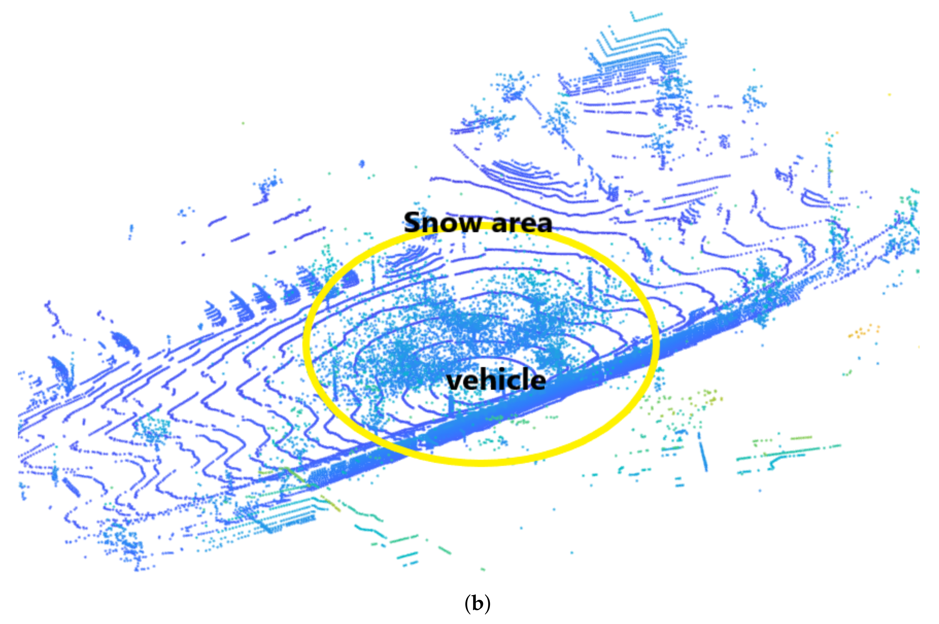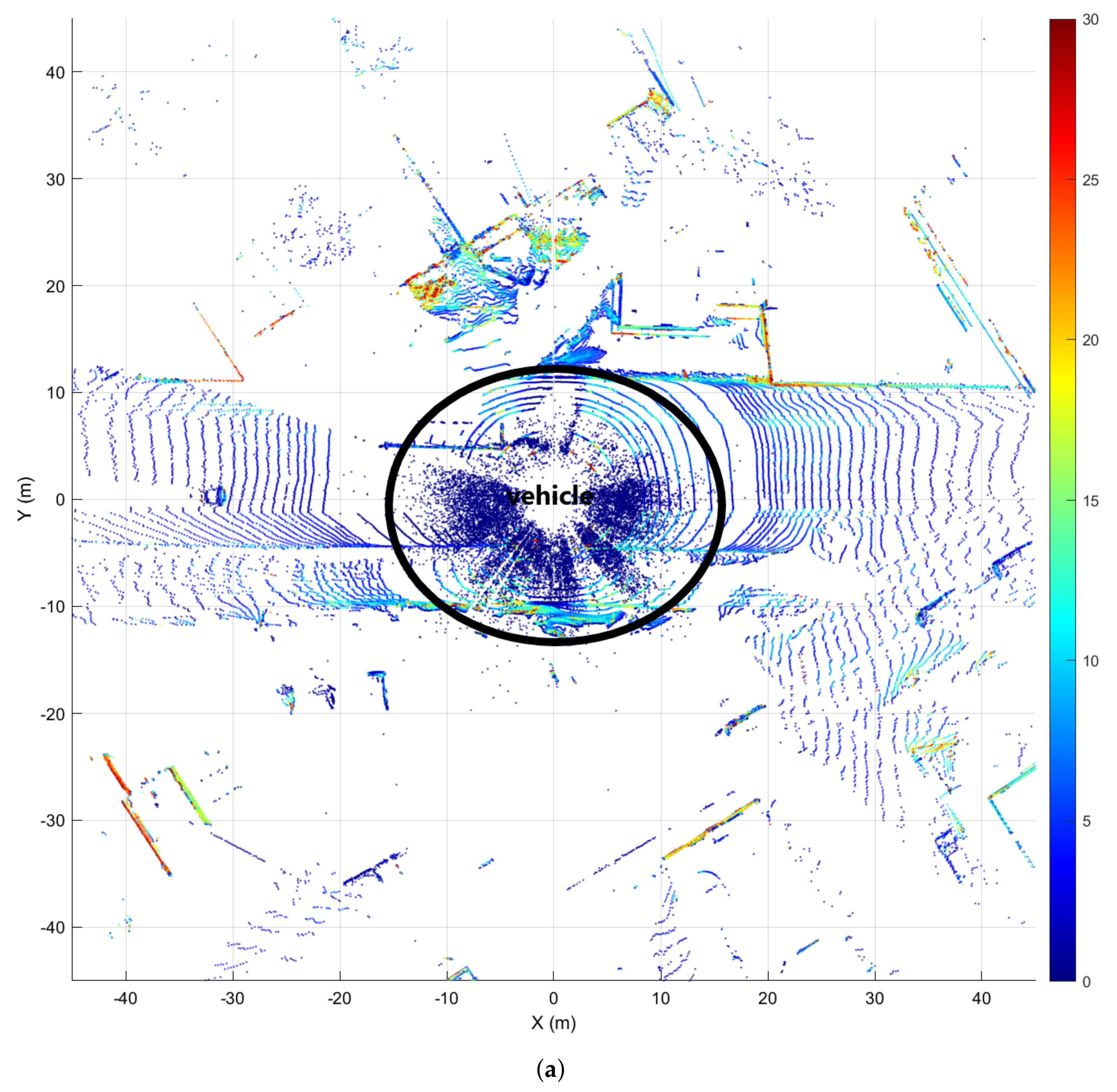That is why numerous studies have focused on LiDAR sensors with the primary purpose of improving performance and reliability or solving some of the remaining problems in harsh weather [14,15,16,17,18,19,20]. Data processing from LiDAR has been of interest in recent years. The LiDAR frame under normal weather is shown in Figure 1a on the Panda dataset [21]. Under normal environmental conditions, LiDAR can improve visibility and increase the reliability of autonomous vehicle systems. However, LiDAR’s performance is significantly affected by the environment. Inclement weather can create serious interference with the LiDAR system [22]. LiDAR’s field of vision is also limited and its reliability is reduced. Figure 1b illustrates the effect of weather on LiDAR data from the Canadian Adverse Driving Conditions Dataset [23]. From this figure, there are many points of snowflakes that were captured around the vehicle. This will limit visibility and seriously affect deep learning models. These snow particles appear randomly and interfere with the vehicle’s warning systems. More seriously, the closer the snowflakes appear, the denser they become. This situation can be the main cause of serious accidents in autonomous vehicles. Therefore, filtering noise for data from LiDAR, especially removing snow particles, is an important task to obtain better data.

Currently, there are many filters that can remove noise from collected data. However, the data from LiDAR have certain differences. Designing a separate filter for LiDAR data is necessary to improve the efficiency of the processing time. Noise filters for LiDAR have been designed to solve this problem [17,19,20,24,25,26]. Only a few of them focus on the noise caused by snow particles [18,27,28]. The effect in these designs is very impressive in removing snow points from LiDAR. However, filters also inadvertently remove points that belong to objects. This causes most of the useful information from LiDAR to be lost. Therefore, in this study, we propose an adaptive filter to overcome the disadvantages of the previous filters.

To our knowledge, snow filters often use private datasets that are manually labeled to evaluate. Furthermore, the datasets used for testing are small. In this paper, we propose an Adaptive Group of Density Outlier Removal (AGDOR) filter that can improve accuracy and processing time. The existing data from the Winter Adverse Driving Dataset (WADS) [29] was utilized to evaluate the performance of our proposed filter. The contributions of the research presented in this paper are as follows:

1.

We proposed an adaptive group of density outlier removal filter that can achieve high performance in processing time and accuracy;

2.

We analyze the influence of the parameters in the filter and give the optimal parameters for the filter to work effectively;

3.

We evaluate the accuracy of the AGDOR method based on the Winter Adverse Driving Dataset under snowy weather and compare it with other methods.

2. Related Work

Under extreme weather conditions such as rain and snow, the data obtained from LiDAR are affected by noise [17]. Nowadays, filters capable of removing noise are increasingly being developed to obtain high quality data from LiDAR. Many studies have proposed to reduce the noise in the data. These noise filtering methods can rely on the characteristics of the dataset to identify outliers. There are two classical methods that deliver high efficiency on a LiDAR dataset: radius outlier removal (ROR) and statistical outlier removal (SOR) [30,31]. Based on the clustering characteristic from LiDAR’s data, these filters are quite effective in detecting outliers. ROR searches for all points that are within the range of the search radius (SR). The points will then be classified on the number of points within the search range. The SOR theory is close to that of ROR. SOR detects outlier points that are farther away from their neighbors compared to the average for the point clouds. These two outlier detection methods have the advantage of being suitable for density-based data types.

In traditional filters, the search radius is fixed, while the density of the LiDAR point clouds varies on distance. To obtain a high noise rejection ratio, the filter also removes points from objects. Therefore, the false positive rate of the two methods is extremely high with the LiDAR point clouds. A dynamic radius outlier removal (DROR) [18] was proposed to overcome the limitations of traditional filters. DROR uses a variable search radius to improve the detection of outliers. Since the density of an object’s point clouds will gradually decrease with the distance from the LiDAR to the objects, this improvement makes the filter more efficient. The search radius is determined based on the distance to the object multiplied by a specified multiplier constant. The DROR results show that the proposed method achieves an accuracy of more than 90% on LiDAR point clouds without removing environmental features.

In another approach, noise filters are designed using deep learning models. Weathernet is one of the popular models for LiDAR noise detection from LiDAR point clouds [27]. It was introduced as a de-noising algorithm based on LiLaNet and is representative of approaches using convolutional neural networks. WeatherNet will modify for noise removal purposes by decreasing the number of output layers. In some situations, the effect of using deep learning is better when compared to the traditional approach. However, learning models use significant processing time because they are built from many convolutional layers. Low intensity outlier removal (LIOR) was proposed to improve accuracy and speed for point clouds de-snowing based on the distinction between snow points and non-snow points from LiDAR data [32]. The intensity threshold was determined and applied in the first step. Snow points were detected and removed as outliers on low intensity from this filter. At the second step, an outlier removal filter was applied to save some object points that were classified as outliers from the first step. However, LIOR can be adversely affected under certain conditions. Optimizing the LIOR filter in each condition can reduce the false positive rate characteristics. Hence, Dynamic Distance–Intensity Outlier Removal (DDIOR) was introduced to address this limitation [33]. DDIOR is an enhanced version that overcomes limitations from DSOR. To improve the Precision value, the author used a dynamic distance coefficient and intensity to calculate the dynamic filtering threshold. Statistical outlier removal was used to classify snow particles.

Although DDIOR has significant improvements in snow particles recognition, the filter’s processing time and efficiency are still limited. In particular, a low Precision value is evidence that a significant important data were removed during the filtering process. We proposed Adaptive Group of Density Outlier Removal (AGDOR) to improve accuracy and execution time. Our proposed filter can improv accuracy by more than 96% and uses 0.5 s per frame in execution time from the WADS. The proposed filter can skip the object points based on the improvements in Radius Outlier Removal, which is an especially crucial factor in the autonomous driving system. Moreover, our proposed filter can label multiple points in one cycle of search. Hence, the execution time will be improved.

3. The Proposed Filter

Our proposed filter included two parts: the intensity filter and the radius outlier removal algorithm. The general structure includes a two stages filter to separate snow particles from objects included in the LiDAR dataset. The detailed operation of each stage is described below.

3.1. Intensity Filter

To detect snow spots, a signal strength filter is applied in the first stage to remove most of the high intensity points. Each point in WADS contains four data fields: [X, Y, Z, Intensity]. The intensity of the points was calculated based on the response of the signal of the light beams emitted by the LiDAR. The response of the LiDAR beam is different based on the object’s construction material [34]. In particular, the feedback signal from the snow particles to the LiDAR is incredibly low [35,36]. Taking advantage of this property from snow particles, we propose an intensity-based filter as the first layer. The difference in intensity between the snow particles and the object is depicted in Figure 2a. Snow particles appear densely within 10 m around the LiDAR and gradually decrease with greater distance. The intensity from the snow particles is also extremely low, which is shown in dark blue. The histogram is given to compare the difference in intensity between the object points and the snow points. From Figure 2b, we can easily observe that most of the snow particles are of almost zero intensity.

To define the threshold for the filter, we randomly selected LiDAR frames that have been labeled from the dataset and extract them into two groups. The first group is the set of all point clouds labeled as snow $\left(PcS\right)$, and the other group is the remaining points representing the point clouds of objects $\left(PcO\right)$. Then, the mean $\mu$ of each group was calculated based on the intensity I and the total number of points in each group by Equations (1) and (2):

$${\mu }_{PcS}=\frac{\sum I_{PcS}}{N},$$

(1)

$${\mu }_{PcO}=\frac{\sum I_{PcO}}{M},$$

(2)

where N is the total number of point clouds from $PcS$ and M is the total number of point clouds from $PcO$.

The threshold intensity between two groups of filters is determined based on Equations (1) and (2) according to the formula:

$$I_{th}=\frac{1}{2}({\mu }_{PcO}-{\mu }_{PcS}).$$

(3)

The result from Equation (3) is used as the threshold of intensity to apply to the filter. The set of point clouds $P=\{p_1,p_2,\dots ,p_n\}$ was classified according to the following equation:

$$P=\left\{\begin{array}{cc}{P}_{Low}\hfill & \mathrm{if}{I}_p\le I_{th}\hfill \\ P_{High}\hfill & \mathrm{if}{I}_p>Ith\hfill \end{array}\right.,$$

(4)

where $I_p$ represents the intensity of points in P.

The results after applying the intensity filter are simulated in Figure 3. Points from $P_{High}$ contain only the points that represent objects. Therefore, we label all points in P as inliers. Unfortunately, points in $P_{low}$ contain not only snow particles, but also non-snow particles. Therefore, we propose to filter out the non-snow particles from $P_{low}$ in the second stage.

3.2. Adaptive Group of Density Outlier Removal Filter

The second stage detects snowflakes from $P_{Low}$. We found that the snow particles appear randomly. Therefore, their density is sparser than that of objects. Objects appear in clusters, while snow particles appear randomly out of order. Moreover, the distance between points in the LiDAR will tend to become sparse with longer distances. Based on the above characteristics of the LiDAR dataset, an AGDOR filter was proposed to detect snow particles in $P_{Low}$. The set $F(F\in P_{Low})$, which is called the nearest neighbor, was recognized based on the search radius $\left(SR\right)$ by the following formula:

$$F_i=p_0\in P_{Low}\mid dist(p_i,p_0)<=SR,$$

(5)

where $p_0$ is the set of points whose distance to $p_i$ is less than the search radius (SR) and $dist(p_i,p_0)$ is the Euclidean distance from $p_i$ to $p_0$. In response to variation in density of point clouds in the LiDAR data, we used a variable search radius; a dynamic $SR$ is determined by the formula:

$$SR=\alpha \times \theta \times dist,$$

(6)

where $\alpha$ is the multiplier of minimal distance at the point $p_0$, $\theta$ is the angular resolution $\left(azimuth\right)$ of LiDAR and $dist$ is the Euclidean distance from $p_i$ to LiDAR. $\theta$ is different depending on the LiDAR model. $SR$ is a graph that varies with distance. $\alpha$ and $\theta$ are constant, so we can call $Mul=\alpha \times \theta$ as a multiplier.

Then, the total points $N_{F_i}$ were counted from the set $F_i$. Core points and outlier were identified based on numbers of neighbor $\left(NoN\right)$ and $N_{F_i}$:

$$F_i=\left\{\begin{array}{cc}{P}_{i\_Core}\hfill & \mathrm{if}NoN\le N_{F_i}\hfill \\ P_{i\_Outlier}\hfill & \mathrm{if}NoN>N{F}_i\hfill \end{array}\right..$$

(7)

The peculiarity of our method is to group all neighboring points of $p_i$$\left(F_i\right)$ and label them as inliers if $p_i$ is a core point. Therefore, our proposed method reduces the computation time. The idea of our proposed filter is illustrated in Figure 4. The blue points, red points, and white points represent border points, core points, and outlier points, respectively. Border points are labeled on the search radius of the points that are considered core points. A considerable number of points are labeled based on this idea. The filter calculation time is effectively simplified. From the example in Figure 4, 10 points are marked as inliers while we only use three steps for the search. Using this idea, the filter performance is significantly improved.

We also designed an input checker in the second stage to determine whether the points were labeled or not. Our method is to group objects neighboring the core point, so there is no need to check all points from the input. The overall flow of our filter is shown in Algorithm 1.

Algorithm 1 Pseudocode of our proposed filter

Input:  $P=p_1,p_2,...,p_n$; $p_i=x_i,y_i,z_i,I_i$ Output:  $P_{snows}$,$P_{Objects}$       Stage1: Intensity filter 1: for$p\in P$do 2:    $I_{th}=\frac{1}{2}({\mu }_{PcO}-{\mu }_{PcS})$ 3:    if $I_p<I_{th}$ then 4:        point p classified as $P_{Low}$ 5:    else 6:       point p classified as an object (inlier) 7:    end if 8: end for 9: return$P_{Low}$ Stage 2: Adaptive group of density outlier removal filter 10: for$p\in P_{Low}$do 11:    if $P_i$ was not labeled then 12:        $dist=\sqrt{(x_i^2+y_i^2+z_i^2)}$ 13:        $SR=\alpha \times \theta \times dist$ 14:        $F_i\leftarrow KDTreeSearchRadius\left(SR\right)$ 15:        Count the number of $F\left(N_{F_i}\right)$ 16:        if $NoN\le N_{F_i}$ then 17:           $F_i\leftarrow$ Object points (inlier) 18:       else 19:         $P_i\leftarrow$ Snow point (outlier) 20:      end if 21:    end if 22: end for

4. Performance Analysis

To demonstrate the reliability of the proposed method, we conducted experiments on the Winter Adverse Driving Dataset. The experimental results are also compared with other methods on the same dataset. In this chapter, we will briefly present information about the dataset in part one. The quality of the filter is evaluated in part two by comparing the results of the experiment with the ROR, SOR, DROR, and LIOR methods.

4.1. Experimental Dataset

To the best of our knowledge, the Winter Adverse Driving Dataset is the first open dataset that is labeled with snow particles on each point cloud. Each point in the dataset is labeled with a total of 22 classes. In our experiment, active falling snow is used to demonstrate the quality of the filter, and the other classes in the dataset are grouped into groups of objects. Moreover, this dataset contains a large number of frames that have been carefully labeled with snow particles. There are nineteen scenes in the dataset, each of which contains approximately 100 frames. Each frame provides more than 200,000 points. The weather conditions in the dataset have considerable diversity, such as light, medium, heavy, and extreme snow fall. Furthermore, the datasets in previous research are not comprehensive due to the lack of data, and are heterogeneous. Therefore, this dataset is suitable to demonstrate the effectiveness as well as the generality of the proposed model.

4.2. Comparison of Outlier Filters

We implemented five different filters in this experiment: ROR, SOR, DROR, LIOR, and our proposed filter (AGDOR). Four filters use the same dataset and programming language. Multiplier $\left(\alpha \right)$ and number of neighbor $\left(NoN\right)$ are two parameters that affect the result of the filter. The choice of parameter $\alpha$ depends on the density of the point clouds. In this experiment, we use a parameter $\alpha$ with a value varying from 0.005 to 0.04 and $NoN$ with a value varying from 4 to 8 to investigate the influence of these two parameters on the quality of the filter. From the results of this experiment, we can find the optimal parameter for the filter. Our experiments were conducted with the open3D package [37] from the Python language. A workstation with an Intel® Xeon® Silver 4114 CPU @2.20 GHz, GRID Virtual GPU V100D-8Q, and 32 GB RAM memory was utilized in our experiment.

The filter parameters of our experiment are shown in

Table 1. Filter parameters.

Method	Parameters	Values
ROR	Min. number of neighbors	5
	Search radius	0.1 m
SOR	Number of neighbors	5
	Standard deviation	0.1
DROR	Search radius	5
	Radius multiplier	3
	Azimuth angle	0.1${}^{\circ }$
LIOR	Search radius	0.1 m
	Min. number of neighbors	5
	Snow detection range	71.235 m
	Intensity threshold constant	9
DSOR	Number of neighbors	5
	Multiplicative factor	0.05
	Global threshold constant	0.1
DDIOR	Number of neighbors	5
AGDOR	Min. number of neighbors	5
	Multiplier factor	0.001
	Intensity threshold constant	9

. To ensure fairness, we chose the optimal parameters from previous studies. In this study, we have some small adjustments such as azimuth resolution (DROR), threshold intensity (LIOR), search radius (ROR and LIOR). Differences in dataset and LiDAR model are the reasons for these adjustments. We also use results from Wang et al. (2022) to compare with our proposed filter.

4.3. Evaluation Metrics

Each filter result contains four basic parameters including True Positive $\left(TP\right)$, True Negative $\left(TN\right)$, False Positive $\left(FP\right)$, and False Negative $\left(FN\right)$. In this study, $TP$ represents the number of correctly predicted snow particles, $TN$ represents the number of correctly predicted object points, $FN$ represents the number of falsely predicted snow particles, and $FP$ represents the number of object points that were predicted incorrectly. A well-defined noise filter is one that can find a large amount of snow (high $TP$) while preserving valuable information from the objects (low $FP$). Moreover, the filter processing speed is also an important feature for comparison. Therefore, five metric systems were used to evaluate performance in this study including Execution time, Accuracy $\left(Acc\right)$, Precision $\left(Pre\right)$, Recall $\left(Re\right)$, and F1-score $\left(F1\right)$. The data used in the experiment is unbalanced data. Each frame contains 8000–30,000 snow points per over 200,000 point clouds. $Pre$ and $Re$ are two common metrics used to solve the above problem. However, a trade-off between $Pre$ and $Re$ always occurs in most cases, $F1$ is suggested as a balance between the two metrics. These metrics are calculated according to the formulas below:

$$Acc=\frac{TP+TN}{TP+TN+FP+FN},$$

(8)

$$Recall=\frac{TP}{TP+FN},$$

(9)

$$Pre=\frac{TP}{TP+FP},$$

(10)

$$F1=\frac{Pre\times Re}{Pre+Re}.$$

(11)

4.4. Implementation Results

Determining the value of the parameters in the filter is necessary to enhance the filter’s ability to recognize noise points. Figure 5 simulates the impact of the multiplier and number of neighbors on the results. $Acc$ and $F1$ have almost the same variation. The highest accuracy in Figure 5, of 96.16%, was achieved when the multiplier is 0.01 and the NoN is 4. The highest $F1$ in Figure 5 of 83.3% appears when the multiplier is 0.01 and the NoN is 5. If we increase the multiplier, the NoN needs to increase to obtain the optimal result. However, the filter efficiency will reduce with high multipliers, even if we used the corresponding NoN. The multiplier will lead to an increase in the search radius. A large search radius will accidentally contain snow particles. Results obtained from a high multiplier do not have ideal performance. Hence, we use a multiplier of 0.01 and a NoN of 5 as an optimal value for the filter for compare with another research. Execution time also needs to be considered in our experiment. Filter processing time tends to increase as we decrease the search radius or increase min number of neighbors. The number of neighboring points will increase as the search scope increases. When defining a core point, there will be many labeled neighbors without the need for an algorithm to determine their labels.

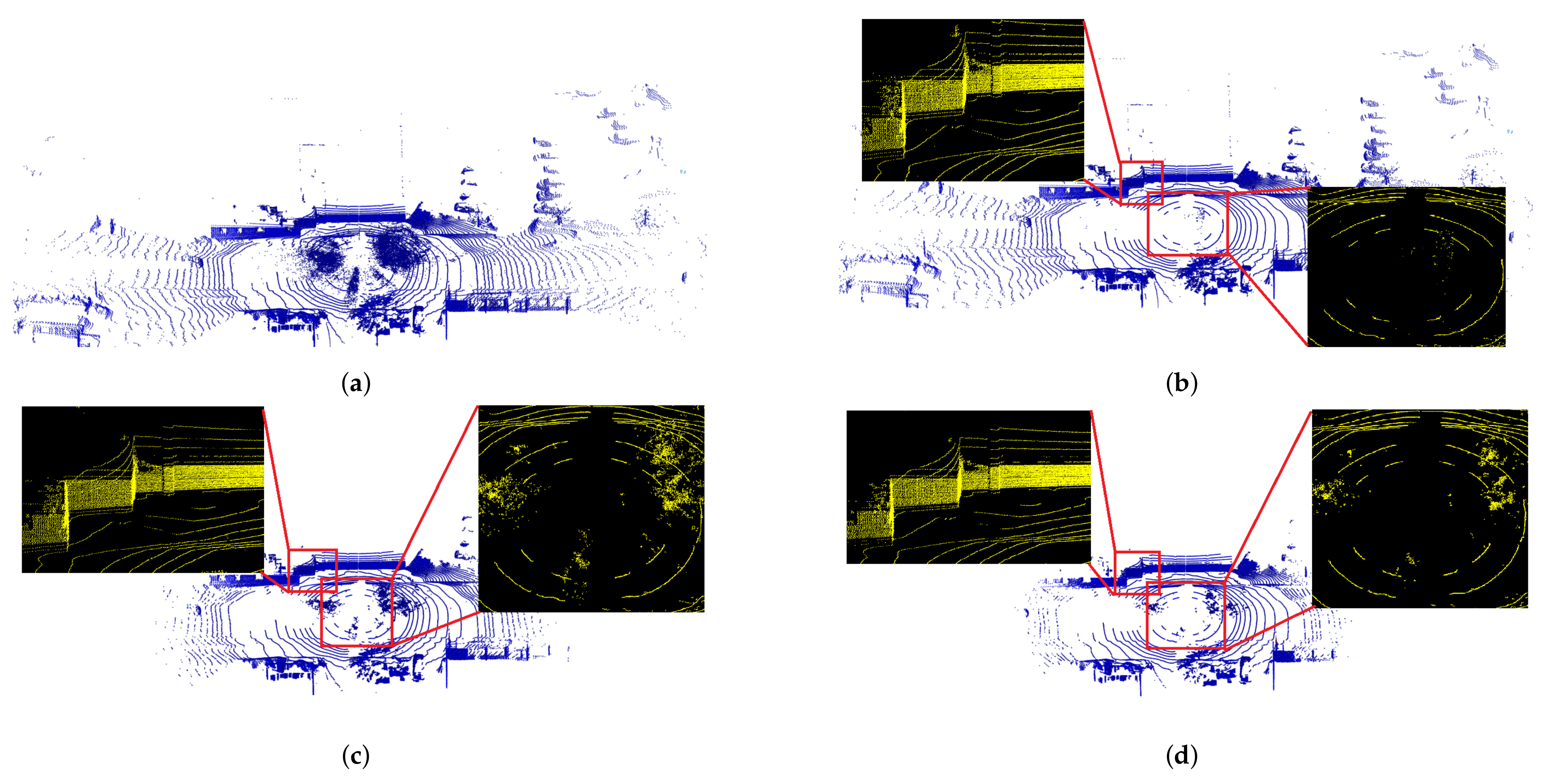
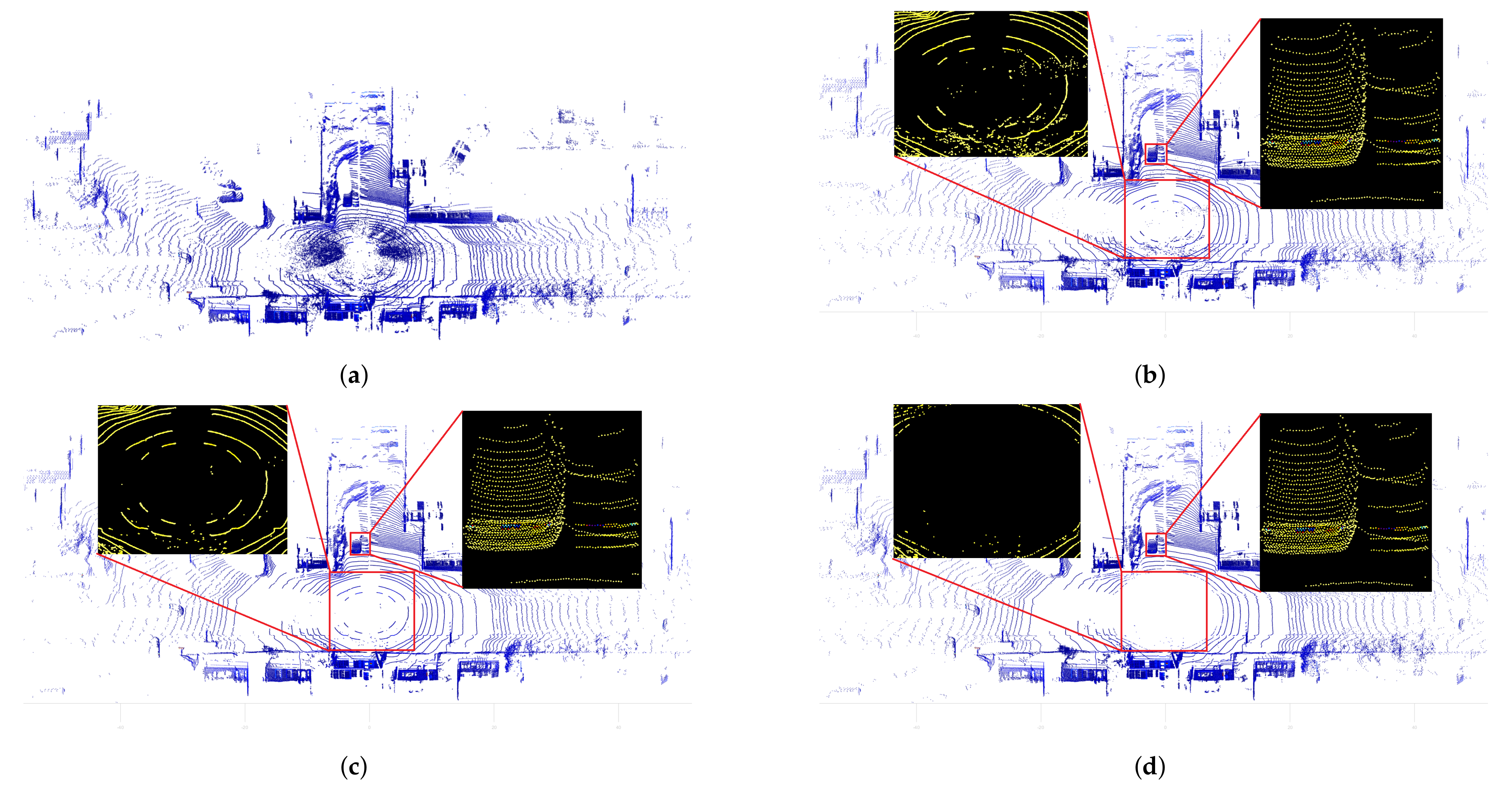
The results of the application of the proposed filter are presented in Figure 6 and Figure 7. The first images are the raw point clouds from the WDS dataset, while the second images show the ground truth, and the final image shows the result after snow removal with our proposed filter. There are many snow particles that appear around the vehicle that were collected by LiDAR in Figure 6a. To prove the performance stability of our proposed method, we visualized Figure 7 in light snowfall. The clear frame is shown in Figure 6b and Figure 7b after removing snow points from the ground truth. The results of our algorithm and the four comparison methods are also presented.

The snow particles appear dense in Figure 6a under heavy snowfall conditions. The density of point clouds from the LiDAR data is sensitive to distance. Therefore, it is difficult for traditional density-based filters to be effective in detecting snowflakes. The two traditional filters that failed to remove the noise are demonstrated in Figure 6c,d. Since the filter does not have the density adjustment, the long-distance information is missing after applying the filter. LIOR, DROR, and DSOR work more efficiently and are shown in Figure 6e–g, respectively. Most of the key characteristics of the data are retained. However, the ability to filter noise comes at the trade-off of the retention of important data points. The higher the efficiency in snow detection, the more important data points are lost. Our proposed model overcomes this limitation. The results of AGDOR are simulated in Figure 6h and Figure 7f. Compared to the ground truth, our method can obtain high accuracy. The zoom regions from Figure 7 show that our proposed method can retain more feature points when compared with other methods. The high density of snow particles was effectively removed, while most of the crucial information of the objects was preserved. Objects around the vehicle are easily observed with the effectiveness of the filter. The input data from LiDAR has been cleaned without losing key features in heavy snow conditions.

4.5. Effectiveness of AGDOR

In this section, the filter performance is evaluated by comparing processing time and accuracy with the SOR, ROR, DROR, and LIOR filters. The results in

Table 2. Comparison of the proposed filter.

Filters	$\mathit{Acc}(\%)$	$\mathit{Pre}(\%)$	$\mathit{Recall}(\%)$	$\mathit{F}1(\%)$	Execution Time (s)
SOR	79.57	32.73	21.96	26.98	0.21
ROR	62.5	67.79	18.19	28.68	0.25
LIOR	90.35	66.17	55.56	60.4	0.07
DROR	96.17	71.91	91.89	80.68	10.99
DSOR	95.77	65.07	95.6	77.43	0.2
DDIOR	96.26	69.87	95.23	80.6	1.3
AGDOR	96.15	86.19	80.59	83.3	0.51

provide an overview of the filter’s efficiency.

Accuracy $\left(Acc\right)$, Precision $\left(Pre\right)$, Recall $\left(Re\right)$, and F1-score $\left(F1\right)$ were calculated and analyzed in detail. Traditional filters failed to detect snow particles. However, the processing time of these filters is faster than other filters because of simple structure. The LIOR filter has a significant advantage in Recall over the traditional method. Intensity-based filters in the first step are more effective in reducing false positive rates. Unfortunately, the radius outlier removal in the second step is not effective in classifying data point clouds of low intensity. The DROR, DSOR, and DDIOR filters have higher Precision and Recall than LIOR. However, the DROR, DSOR, and DDIOR filters also have a high ratio of $FN$, which means that many object points were detected as snow points. This disadvantage causes significant essential information of the LiDAR to be lost, affecting object recognition that ensures the safety of vehicle drivers.

Our method has a significant improvement in Precision. The Accuracy of our proposed filter increased by 16.58%, 33.65%, 5.8%, and 0.38% over SOR, ROR, LIOR, and DSOR, respectively. However, our proposed filter has a smaller value on accuracy than DROR and DDIOR. In particular, the Precision from the AGDOR method outperforms the other methods, with increases of 47.46%, 18.4%, 20.02%, 14.28%, 21.12%, and 16.32% over SOR, ROR, LIOR, DROR, DSOR, and DDIOR, respectively. This information demonstrates that the feature points are not removed after applying the filter. Hence, the F1-score was significantly increased by 56.32%, 54.62%, 22.9%, 2.62%, 5.87%, and 2.7% over SOR, ROR, LIOR, DROR, DSOR, and DDIOR, respectively. Important data from LiDAR was preserved by our method, which is visualized in Figure 7. Due to using the method of grouping objects, the proposed method is highly effective in retaining the object points at the edges of the objects. However, this method has difficulty detecting snow points near objects. This is a major limitation of this method. We believe that the True Positive and False Positive trade-off is balanced by the F1-score. Therefore, F1-score is an important parameter in filter evaluation. The proposed method has a significantly higher number of results than those of the compared filters.

The processing time is also reported in Table 2. The object points are significantly removed in the first stage of the filter. Hence, AGDOR achieves very impressive results in processing time when compared to the state-of-the-art methods. AGDOR is 2.5 times faster than DDIOR in execution time. Moreover, the points grouping method proved to be effective in reducing execution time. However, our filter is two times slower compared to LIOR, DSOR, and traditional filters.

5. Discussion

The data from LiDAR is clustered; however, the density of the clusters is variable based on the distance to the vehicle. Therefore, our proposed adaptive filter is more effective in detecting snow particles than traditional methods using only fixed parameters. Adaptive filtering methods require significant execution time, which is shown in the DROR filter. Hence, an intensity filter is applied to remove a large number of object points to improve the processing time and the accuracy of the filter, as shown in the LIOR method. However, the special feature of our method is the grouping of objects. Not only core points, but also border points were labeled. Object points located at the edge are classified more accurately on this filter. Therefore, the Recall of the recommendation filter is significantly higher with that of other methods. Based on the results obtained from the experiment, AGDOR solved two main problems: the ability to detect snow points in extreme snow conditions and improved processing time on high resolution data frames.

Our proposed method has an outstanding Precision coefficient. This confirms its lower rate of missing object points than other filters. The more object points are retained, the more reliable are the sensors in vehicles. The accuracy of AGDOR is the highest among the comparison methods, so it can be used very effectively in a high-noise environment. Furthermore, the obtained results were validated on the WADS, which has approximately 18,000 frames (18 sequences; each sequence has about 100 frames) to ensure the reliability of the proposed method. The experimental data suggest that AGDOR is very suitable for removing noise from LiDAR, especially snowflakes.

Along with the development of sensor technology, the data obtained from LiDAR is huge. One of the most challenging problems in this area is execution time. The method of grouping objects was proposed to improve execution time. Unfortunately, our proposed filter has twice the processing time of traditional methods and is impossible with real-time systems. Therefore, methods such as data dimensionality reduction are considered for future improvement. Another limitation in this study is the selection of parameters of the filter. To solve this problem, the optimal value for the filter was determined based on detailed analysis of the influence of the parameters on the filter results.

6. Conclusions

The results of our proposed method provide valuable insight into the outstanding performance of the proposed model. Working well in extreme environments has been a challenging task in recent studies. Experiments from the WADS confirm that the algorithm is highly effective in reducing snow points during data collection. This is necessary for the combination of an intensity filter and a density filter. In some cases, the $TP$ is lower than the recent filter. We believe that there is always a trade-off between the $TP$ rate and the $FN$ rate. After applying the proposed filter, the obtained F1-score and Accuracy are higher under all conditions of weather. The point clouds after the two-stage filter were completely clear. With a F1-score above 83%, our proposed method is satisfactory in many cases, especially for vehicle driver assistance systems. We believe that the accuracy is always more than 95%, which is ideal for a combination model. This study has shown that the AGDOR filter is faster while providing similar performance when compared with other methods, such as DDIOR. Furthermore, our proposed filter is capable of retaining important information from obstacles. The combination of two stages filter can help LiDAR operate more efficiently, as well as improve the efficiency in extreme environments. This could be a new direction for filtering noise from LiDAR point clouds and a new pre-processing approach to machine learning.

References

- Martínez-Díaz, M.; Soriguera, F. Autonomous vehicles: Theoretical and practical challenges. Transp. Res. Procedia 2018, 33, 275–282. [Google Scholar] [CrossRef]
- Fayyad, J.; Jaradat, M.A.; Gruyer, D.; Najjaran, H. Deep learning sensor fusion for autonomous vehicle perception and localization: A review. Sensors 2020, 20, 4220. [Google Scholar] [CrossRef] [PubMed]
- Yeong, D.J.; Velasco-hernandez, G.; Barry, J.; Walsh, J. Sensor and sensor fusion technology in autonomous vehicles: A review. Sensors 2021, 21, 2140. [Google Scholar] [CrossRef] [PubMed]
- Wen Hu, J.; Yin Zheng, B.; Wang, C.; Hui Zhao, C.; Lei Hou, X.; Pan, Q.; Xu, Z. A survey on multi-sensor fusion based obstacle detection for intelligent ground vehicles in off-road environments. Front. Inf. Technol. Electron. Eng. 2020, 21, 675–692. [Google Scholar] [CrossRef]
- Zhong, Z.; Liu, S.; Mathew, M.; Dubey, A. Camera radar fusion for increased reliability in ADAS applications. Electron. Imaging 2018, 2018, 258-1–258-4. [Google Scholar] [CrossRef]
- Kang, D.; Kum, D. Camera and Radar Sensor Fusion for Robust Vehicle Localization via Vehicle Part Localization. IEEE Access 2020, 8, 75223–75236. [Google Scholar] [CrossRef]
- Caesar, H.; Bankiti, V.; Lang, A.H.; Vora, S.; Liong, V.E.; Xu, Q.; Krishnan, A.; Pan, Y.; Baldan, G.; Beijbom, O. Nuscenes: A multimodal dataset for autonomous driving. In Proceedings of the IEEE/CVF Conference on Computer Vision and Pattern Recognition, Seattle, WA, USA, 13–19 June 2020. [Google Scholar] [CrossRef]
- Kolar, P.; Benavidez, P.; Jamshidi, M. Survey of datafusion techniques for laser and vision based sensor integration for autonomous navigation. Sensors 2020, 20, 2180. [Google Scholar] [CrossRef]
- Yang, J.; Liu, S.; Su, H.; Tian, Y. Driving assistance system based on data fusion of multisource sensors for autonomous unmanned ground vehicles. Comput. Netw. 2021, 192, 108053. [Google Scholar] [CrossRef]
- Li, Y.; Ibanez-Guzman, J. Lidar for Autonomous Driving: The Principles, Challenges, and Trends for Automotive Lidar and Perception Systems. IEEE Signal Process. Mag. 2020, 37, 50–61. [Google Scholar] [CrossRef]
- Bai, L.; Zhao, Y.; Huang, X. Enabling 3D Object Detection with a Low-Resolution LiDAR. IEEE Embed. Syst. Lett. 2022, 1. [Google Scholar] [CrossRef]
- Zhong, H.; Wang, H.; Wu, Z.; Zhang, C.; Zheng, Y.; Tang, T. A survey of LiDAR and camera fusion enhancement. Procedia Comput. Sci. 2021, 183, 579–588. [Google Scholar] [CrossRef]
- Zhen, W.; Hu, Y.; Liu, J.; Scherer, S. A Joint Optimization Approach of LiDAR-Camera Fusion for Accurate Dense 3-D Reconstructions. IEEE Robot. Autom. Lett. 2019, 4. [Google Scholar] [CrossRef]
- Jokela, M.; Kutila, M.; Pyykönen, P. Testing and validation of automotive point-cloud sensors in adverse weather conditions. Appl. Sci. 2019, 9, 2341. [Google Scholar] [CrossRef]
- Wojtanowski, J.; Zygmunt, M.; Kaszczuk, M.; Mierczyk, Z.; Muzal, M. Comparison of 905 nm and 1550 nm semiconductor laser rangefinders’ performance deterioration due to adverse environmental conditions. Opto Electron. Rev. 2014, 22, 183–190. [Google Scholar] [CrossRef]
- Zheng, J.; Xu, B.; Wang, X.; Fan, X.; Xu, H.; Sun, G. A portable roadside vehicle detection system based on multi-sensing fusion. Int. J. Sens. Netw. 2019, 29, 38–47. [Google Scholar] [CrossRef]
- Kutila, M.; Pyykonen, P.; Holzhuter, H.; Colomb, M.; Duthon, P. Automotive LiDAR performance verification in fog and rain. In Proceedings of the 2018 21st International Conference on Intelligent Transportation Systems (ITSC), Maui, HI, USA, 4–7 November 2018. [Google Scholar] [CrossRef]
- Charron, N.; Phillips, S.; Waslander, S.L. De-noising of lidar point clouds corrupted by snowfall. In Proceedings of the 2018 15th Conference on Computer and Robot Vision (CRV), Toronto, ON, Canada, 4–9 May 2018. [Google Scholar] [CrossRef]
- Bijelic, M.; Gruber, T.; Ritter, W. A Benchmark for Lidar Sensors in Fog: Is Detection Breaking Down? In Proceedings of the 2018 IEEE Intelligent Vehicles Symposium (IV), Changshu, China, 26–30 June 2018. [Google Scholar] [CrossRef]
- Heinzler, R.; Schindler, P.; Seekircher, J.; Ritter, W.; Stork, W. Weather influence and classification with automotive lidar sensors. In Proceedings of the 2019 IEEE Intelligent Vehicles Symposium (IV), Paris, France, 9–12 June 2019. [Google Scholar] [CrossRef] [Green Version]
- Xiao, P.; Shao, Z.; Hao, S.; Zhang, Z.; Chai, X.; Jiao, J.; Li, Z.; Wu, J.; Sun, K.; Jiang, K.; et al. PandaSet: Advanced Sensor Suite Dataset for Autonomous Driving. In Proceedings of the 2021 IEEE International Intelligent Transportation Systems Conference (ITSC), Indianapolis, IN, USA, 19–22 September 2021. [Google Scholar] [CrossRef]
- Rönnbäck, S.; Wernersson, Å. On filtering of laser range data in snowfall. In Proceedings of the 2008 4th International IEEE Conference Intelligent Systems, Varna, Bulgaria, 6–9 September 2008; Volume 3. [Google Scholar] [CrossRef]
- Pitropov, M.; Garcia, D.E.; Rebello, J.; Smart, M.; Wang, C.; Czarnecki, K.; Waslander, S. Canadian Adverse Driving Conditions dataset. Int. J. Robot. Res. 2021, 40, 681–690. [Google Scholar] [CrossRef]
- Rasshofer, R.H.; Spies, M.; Spies, H. Influences of weather phenomena on automotive laser radar systems. Adv. Radio Sci. 2011, 9, 49–60. [Google Scholar] [CrossRef]
- Filgueira, A.; González-Jorge, H.; Lagüela, S.; Díaz-Vilariño, L.; Arias, P. Quantifying the influence of rain in LiDAR performance. Meas. J. Int. Meas. Confed. 2017, 95, 143–148. [Google Scholar] [CrossRef]
- Duan, Y.; Yang, C.; Li, H. Low-complexity adaptive radius outlier removal filter based on PCA for lidar point cloud denoising. Appl. Opt. 2021, 60, E1–E7. [Google Scholar] [CrossRef]
- Heinzler, R.; Piewak, F.; Schindler, P.; Stork, W. CNN-Based Lidar Point Cloud De-Noising in Adverse Weather. IEEE Robot. Autom. Lett. 2020, 5, 2514–2521. [Google Scholar] [CrossRef]
- Balta, H.; Velagic, J.; Bosschaerts, W.; Cubber, G.D.; Siciliano, B. Fast Statistical Outlier Removal Based Method for Large 3D Point Clouds of Outdoor Environments. IFAC PapersOnLine 2018, 51, 348–353. [Google Scholar] [CrossRef]
- Kurup, A.; Bos, J. DSOR: A Scalable Statistical Filter for Removing Falling Snow from LiDAR Point Clouds in Severe Winter Weather. arXiv 2021, arXiv:2109.07078. [Google Scholar]
- Aldoma, A.; Marton, Z.C.; Tombari, F.; Wohlkinger, W.; Potthast, C.; Zeisl, B.; Rusu, R.B.; Gedikli, S.; Vincze, M. Tutorial: Point Cloud Library: Three-Dimensional Object Recognition and 6 DOF Pose Estimation. IEEE Robot. Autom. Mag. 2012, 19, 80–91. [Google Scholar] [CrossRef]
- Rusu, R.B.; Cousins, S. 3D is here: Point Cloud Library (PCL). In Proceedings of the 2011 IEEE International Conference on Robotics and Automation, Shanghai, China, 9–13 May 2011. [Google Scholar] [CrossRef] [Green Version]
- Park, J.I.; Park, J.; Kim, K.S. Fast and Accurate Desnowing Algorithm for LiDAR Point Clouds. IEEE Access 2020, 8, 160202–160212. [Google Scholar] [CrossRef]
- Wang, W.; You, X.; Chen, L.; Tian, J.; Tang, F.; Zhang, L. A Scalable and Accurate De-Snowing Algorithm for LiDAR Point Clouds in Winter. Remote Sens. 2022, 14, 1468. [Google Scholar] [CrossRef]
- Kidd, J.R. Performance Evaluation of the Velodyne VLP-16 System for Surface Feature Surveying. Ph.D. Thesis, University of New Hampshire, Durham, NH, USA, 2017. [Google Scholar]
- Li, H.; Liping, D.; Huang, X.; Li, D. Laser intensity used in classification of lidar point cloud data. In Proceedings of the IGARSS 2008–2008 IEEE International Geoscience and Remote Sensing Symposium, Boston, MA, USA, 6–11 July 2008; Volume 2. [Google Scholar] [CrossRef]
- Roy, G.; Cao, X.; Bernier, R.; Tremblay, G. Physical model of snow precipitation interaction with a 3D lidar scanner. Appl. Opt. 2020, 59, 7660–7669. [Google Scholar] [CrossRef]
- Lu, Z.; Guerrero, P.; Mitra, N.J.; Steed, A. Open3D: Crowd-sourced distributed curation of city models. In Proceedings of the 21st International Conference on Web3D Technology, Anaheim, CA, USA, 22–24 July 2016. [Google Scholar] [CrossRef] [Green Version]