
Attentive SOLO for Sonar Target Segmentation

Abstract
:1. Introduction
- (1)
- A new model named Attentive SOLO for sonar image segmentation is designed. The improved attention module of gated fusion pyramid segmentation was used to extract the boundary information of sonar image targets, improving the accuracy of the segmentation results.
- (2)
- A GF-PSA module is designed. The GFF was used to improve the fusion method of PSA, reducing the noise in the PSA module during feature fusion and improving the segmentation accuracy.
- (3)
- A sonar image dataset named STSD for sonar target segmentation is constructed. The sonar dataset was collected by Pengcheng Laboratory in Shenzhen, Guangdong Province, China, in the sea area near Zhanjiang City, Guangdong Province. We annotated the dataset, which contains 4000 real sonar images, eight different object categories and 7077 instance annotations.
2. Related Works
2.1. Instance Segmentation Algorithm
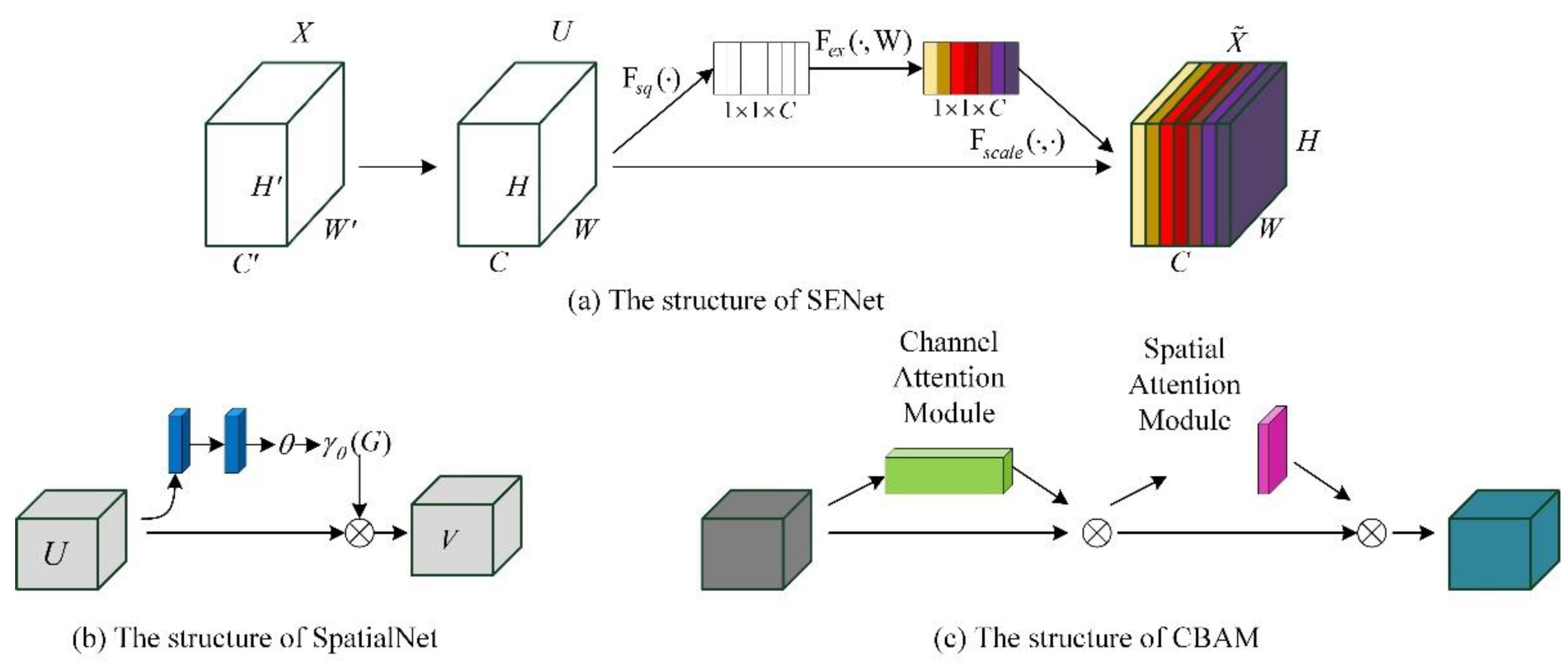
2.2. Attention Mechanism
2.3. Multi-Scale Feature Fusion
2.4. Sonar Datasets
3. Methods
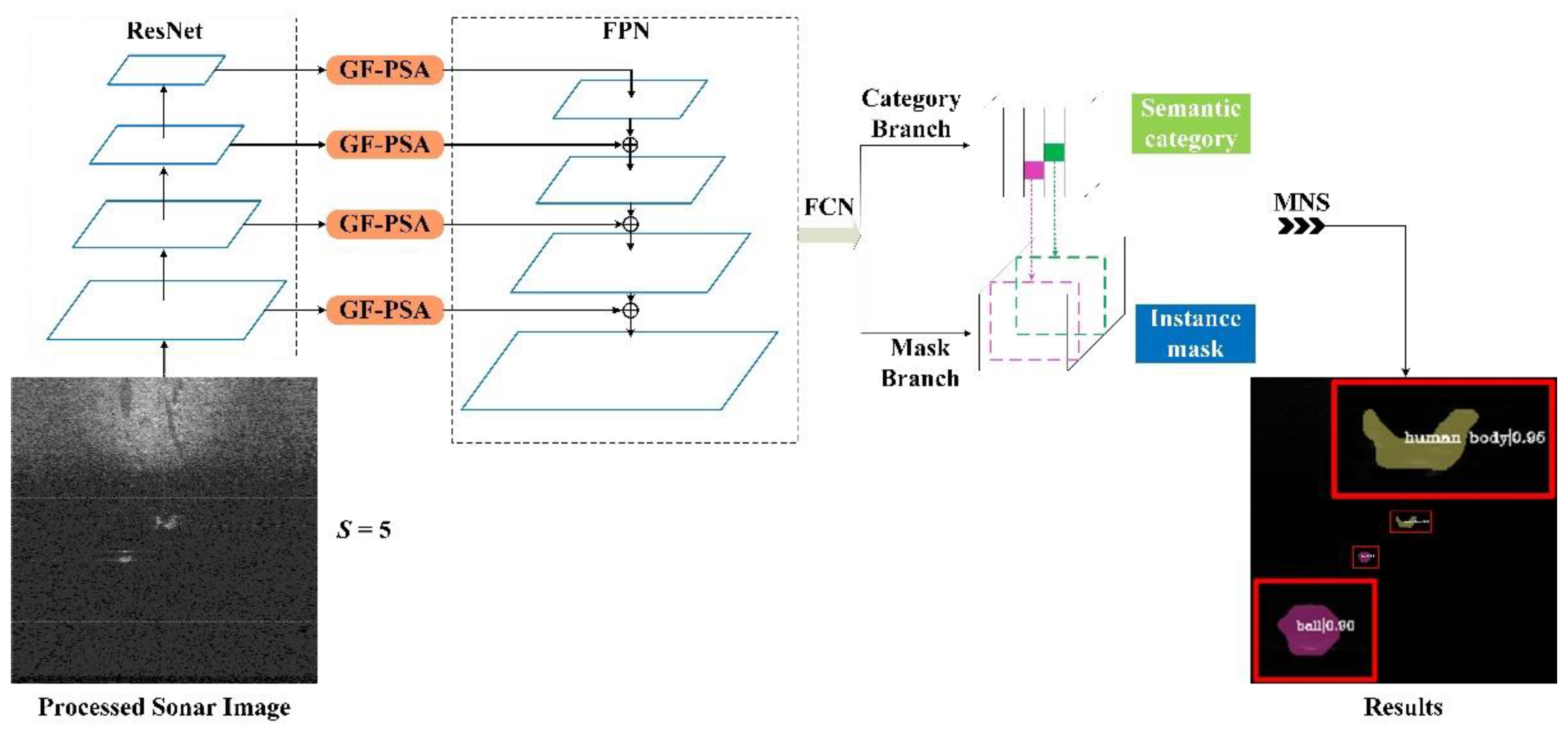
3.1. Attentive SOLO
3.2. Gated Fusion Module
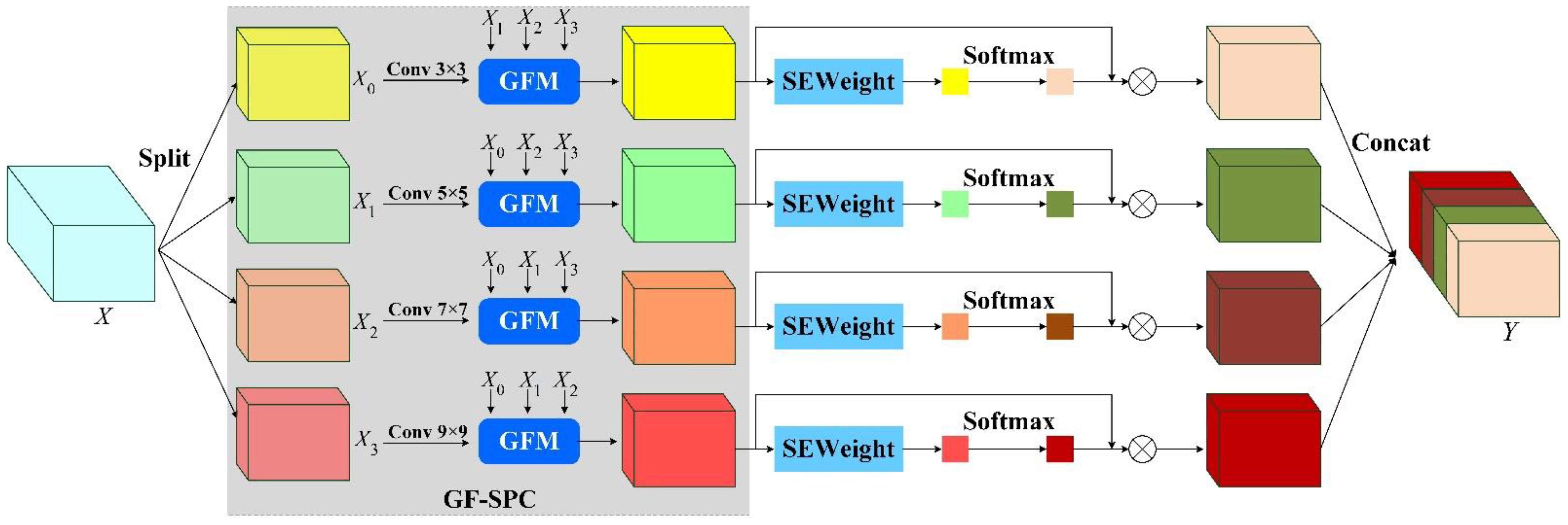
3.3. Gated Fusion-Pyramid Split Attention Block
4. Experiences and Results
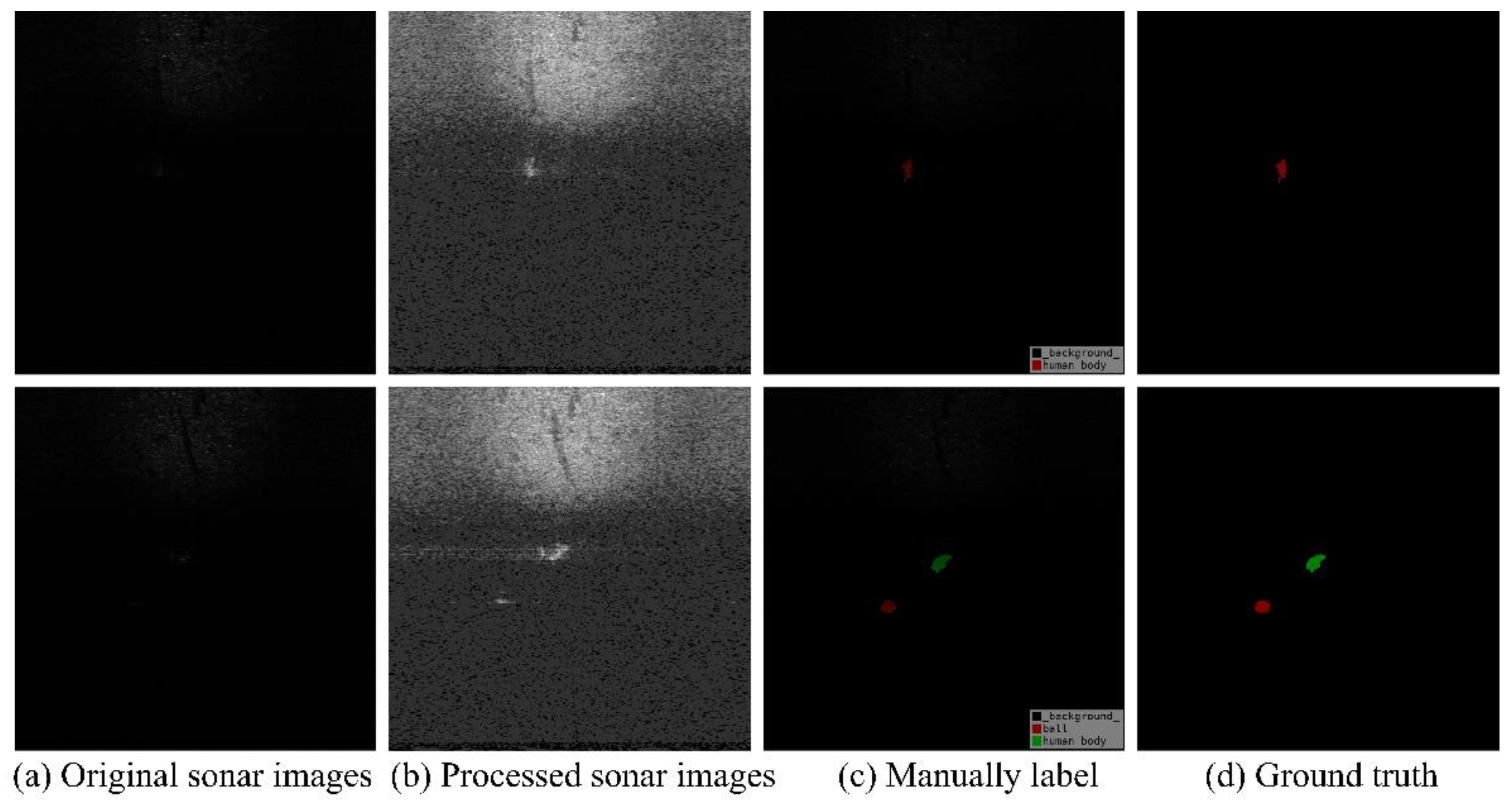
4.1. Dataset
4.2. Implementation Detail
4.3. Evaluation Index
4.4. Ablation Experiments
4.5. Comparative Experiment
5. Conclusions
Author Contributions
Funding
Data Availability Statement
Conflicts of Interest
References
- Chen, Z.; Wang, Y.; Tian, W.; Liu, J.; Zhou, Y.; Shen, J. Underwater sonar image segmentation combining pixel-level and region-level information. Comput. Electr. Eng. 2022, 100, 107853. [Google Scholar] [CrossRef]
- Ye, X.; Zhang, Z.; Liu, P.; Guan, H. Sonar image segmentation based on GMRF and level-set models. Ocean Eng. 2010, 37, 891–901. [Google Scholar] [CrossRef]
- Song, Y.; Liu, P. Segmentation of sonar images with intensity inhomogeneity based on improved MRF. Appl. Acoust. 2020, 158, 107051. [Google Scholar] [CrossRef]
- Abu, A.; Diamant, R. Enhanced fuzzy-based local information algorithm for sonar image segmentation. IEEE Trans. Image Processing 2020, 29, 445–460. [Google Scholar] [CrossRef]
- Wang, X.; Wang, L.; Li, G.; Xie, X. A Robust and Fast Method for Sidescan Sonar Image Segmentation Based on Region Growing. Sensors 2021, 21, 6960. [Google Scholar] [CrossRef]
- Liu, P.; Song, Y. Segmentation of sonar imagery using convolutional neural networks and Markov random field. Multidimens. Syst. Signal Processing 2020, 31, 21–47. [Google Scholar] [CrossRef]
- Zhao, X.; Qin, R.; Zhang, Q.; Yu, F.; Wang, Q.; He, B. DcNet: Dilated Convolutional Neural Networks for Side-Scan Sonar Image Semantic Segmentation. J. Ocean Univ. China 2021, 20, 1089–1096. [Google Scholar] [CrossRef]
- Wu, M.; Wang, Q.; Rigall, E.; Li, K.; Zhu, W.; He, B.; Yan, T. ECNet: Efficient Convolutional Networks for Side Scan Sonar Image Segmentation. Sensors 2019, 19, 2009. [Google Scholar] [CrossRef]
- Wang, Z.; Guo, J.; Huang, W.; Zhang, S. Side-Scan Sonar Image Segmentation Based on Multi-Channel Fusion Convolution Neural Networks. IEEE Sens. J. 2022, 22, 5911–5928. [Google Scholar] [CrossRef]
- Jiao, S.; Zhao, C.; Xin, Y. Research on Convolutional Neural Network Model for Sonar IMAGE Segmentation. MATEC Conf. 2018, 220, 10004. [Google Scholar] [CrossRef]
- Shelhamer, E.; Long, J.; Darrell, T. Fully Convolutional Networks for Semantic Segmentation. IEEE Geosci. Remote Sens. Lett. 2017, 39, 640–651. [Google Scholar] [CrossRef]
- Wang, X.; Zhang, R.; Kong, T.; Li, L.; Shen, C. SOLOv2: Dynamic and Fast Instance Segmentation. Adv. Neural Inf. Processing Syst. 2020, 33, 17721–17732. [Google Scholar]
- Li, X.; Zhao, H.; Han, L.; Tong, Y.; Tan, S.; Yang, K. Gated Fully Fusion for Semantic Segmentation. arXiv 2020, arXiv:1904.01803v2. [Google Scholar] [CrossRef]
- Zhang, H.; Zu, K.; Lu, J.; Zou, Y.; Meng, D. EPSANet: An Efficient Pyramid Split Attention Block on Convolutional Neural Network. arXiv 2021, arXiv:2105.14447v1. [Google Scholar]
- He, K.; Gkioxari, G.; Dollar, P.; Girshick, R. Mask R-CNN. In Proceedings of the IEEE International Conference on Computer Vision, Venice, Italy, 22–29 October 2017; Volume 42, pp. 386–397. [Google Scholar]
- Liu, S.; Qi, L.; Qin, H.; Shi, J.; Jia, J. Path Aggregation Network for Instance Segmentation. arXiv 2018, arXiv:1803.01534v4. [Google Scholar]
- Liu, S.; Jia, J.; Fidler, S.; Urtasun, R. SGN: Sequential Grouping Networks for Instance Segmentation. In Proceedings of the IEEE International Conference on Computer Vision, Venice, Italy, 22–29 October 2017. [Google Scholar]
- Gao, N.; Shan, Y.; Wang, Y.; Zhao, X.; Huang, K. SSAP: Single-Shot Instance Segmentation with Affinity Pyramid. In Proceedings of the IEEE/CVF International Conference on Computer Vision, Seoul, Korea, 27 October–2 November 2019; Volume 31, pp. 661–673. [Google Scholar]
- Joseph, R.; Santosh, D.; Girshick, R.; Ali, F. You Only Look Once: Unified, Real-Time Object Detection. arXiv 2016, arXiv:1506.02640v5. [Google Scholar]
- Bolya, D.; Zhou, C.; Xiao, F.; Lee, Y.J. YOLACT Real-time Instance Segmentation. arXiv 2019, arXiv:1904.02689v2. [Google Scholar]
- Wang, X.; Zhang, R.; Shen, C.; Kong, T.; Li, L. SOLO: A Simple Framework for Instance Segmentation. arXiv 2021, arXiv:2106.15947v1. [Google Scholar] [CrossRef]
- Tian, Z.; Shen, C.; Chen, H.; He, T. FCOS: Fully Convolutional One-Stage Object Detection. arXiv 2019, arXiv:1904.01355v5. [Google Scholar]
- Xie, E.; Sun, P.; Song, X.; Wang, W.; Liang, D.; Shen, C.; Luo, P. PolarMask: Single Shot Instance Segmentation with Polar Representation. arXiv 2020, arXiv:1909.13226v4. [Google Scholar]
- Sofiiuk, K.; Barinova, O.; Konushin, A. AdaptIS: Adaptive Instance Selection Network. arXiv 2019, arXiv:1909.07829v1. [Google Scholar]
- Zhou, T.; Li, J.; Li, X.; Shao, L. Target-Aware Object Discovery and Association for Unsupervised Video Multi-Object Segmentation. In Proceedings of the IEEE/CVF Conference on Computer Vision and Pattern Recognition, Nashville, TN, USA, 19–25 June 2021. [Google Scholar]
- Zhou, T.; Wang, W.; Liu, S.; Yang, Y.; Gool, L.V. Differentiable Multi-Granularity Human Representation Learning for Instance-Aware Human Semantic Parsing. In Proceedings of the IEEE/CVF Conference on Computer Vision and Pattern Recognition, Nashville, TN, USA, 19–25 June 2021. [Google Scholar]
- Xu, F.; Huang, H.; Wu, J.; Jiang, L. Active Mask-Box Scoring R-CNN for Sonar Image Instance Segmentation. Electronics 2022, 11, 2048. [Google Scholar] [CrossRef]
- Hu, J.; Shen, L.; Albanie, S.; Sun, G.; Wu, E. Squeeze-and- Excitation Networks. In Proceedings of the IEEE Conference on Computer Vision and Pattern Recognition, Salt Lake City, GA, USA, 18–22 June 2018; Volume 42, pp. 2011–2023. [Google Scholar]
- Max, J.; Karen, S.; Andrew, Z.; Koray, K. Spatial Transformer Networks. arXiv 2015, arXiv:1506.02025v3. [Google Scholar]
- Woo, S.; Park, J.; Lee, J.; Kweon, I.S. CBAM: Convolutional Block Attention Module. arXiv 2018, arXiv:1807.06521v2. [Google Scholar]
- Sun, J.; Liu, J.; Tian, H.; Li, Y.; Bao, Y.; Fang, Z.; Lu, H. Dual Attention Network for Scene Segmentation. arXiv 2019, arXiv:1809.02983v4. [Google Scholar]
- Hariharan, B.; Arbelaez, P.; Grishick, R. Hypercolumns for Object Segmentation and Fine-grained Localization. In Proceedings of the IEEE Conference on Computer Vision and Pattern Recognition, Boston, MA, USA, 7–12 June 2015. [Google Scholar]
- Ronneberger, O.; Fischer, P.; Brox, T. U-Net: Convolutional Networks for Biomedical Image Segmentation. arXiv 2015, arXiv:1505.04597v1. [Google Scholar]
- Zhang, Z.; Zhang, X.; Peng, C.; Xue, X.; Sun, J. Exfuse: Enhancing feature fusion for semantic segmentation. In Proceedings of the European Conference on Computer Vision (ECCV), Munich, Germany, 8–14 September 2018. [Google Scholar]
- Lin, D.; Ji, Y.; Lischinski, D.; Cohen, D.; Huang, H. Multi-scale context intertwining for semantic segmentation. In Proceedings of the European Conference on Computer Vision (ECCV), Munich, Germany, 8–14 September 2018. [Google Scholar]
- Kong, W.; Hong, J.; Jia, M.; Yao, J.; Cong, W.; Hu, H.; Zhang, H. YOLOv3-DPFIN: A Dual-Path Feature Fusion Neural Network for Robust Real-Time Sonar Target Detection. IEEE Sens. J. 2020, 20, 3745–3756. [Google Scholar] [CrossRef]
- Liu, D.; Wang, Y.; Ji, Y.; Tsuchiya, H.; Yamashita, A.; Asama, H. CycleGAN-based realistic image dataset generation for forward-looking sonar. Adv. Robot. 2021, 35, 242–254. [Google Scholar] [CrossRef]
- Singh, D.; Valdenegro, M. The Marine Debris Dataset for Forward-Looking Sonar Semantic Segmentation. In Proceedings of the IEEE/CVF Conference on Computer Vision and Pattern Recognition, Nashville, TN, USA, 19–25 June 2021. [Google Scholar]
- Li, T.Y.; Goyal, P.; Grishick, R.; He, K.; Dollar, P. Focal Loss for Dense Object Detection. In Proceedings of the IEEE International Conference on Computer Vision, Venice, Italy, 22–29 October 2017; Volume 42, pp. 318–327. [Google Scholar]


| Dataset | Type | Sensor | Image Number | Instance Category |
|---|---|---|---|---|
| MNSD | forward-looking sonar dataset | - | 5002 | 2 |
| SRSD | forward-looking sonar dataset | - | 1016 | 1 |
| Dataset in [37] | forward-looking sonar dataset | - | 2768 | 3 |
| Dataset in [7] | Side-scan sonar dataset | Dual-frequency side-scan sonar | 12,486 | 0 |
| Dataset in [9] | Side-scan sonar dataset | Collected online | 497 | 3 |
| Dataset in [38] | forward-looking sonar dataset | ARIS Explorer 3000 forward-looking sonar | 1868 | 11 |
| STSD | forward-looking sonar dataset | Tritech Gemini 1200i forward-looking sonar | 4000 | 8 |
| The Value of n | Kernel Size | Group Size |
|---|---|---|
| n = 4 | 3 × 3 | 2 |
| 5 × 5 | 4 | |
| 7 × 7 | 8 | |
| 9 × 9 | 16 |
| Target Category | Number | Ratio | Target Category | Number | Ratio |
|---|---|---|---|---|---|
| Human body | 684 | 10% | Metal bucket | 403 | 6% |
| Tire | 852 | 12% | Cube | 1752 | 25% |
| Round cage | 386 | 5% | Sphere | 1943 | 27% |
| Square cage | 655 | 9% | Cylinder | 402 | 6% |
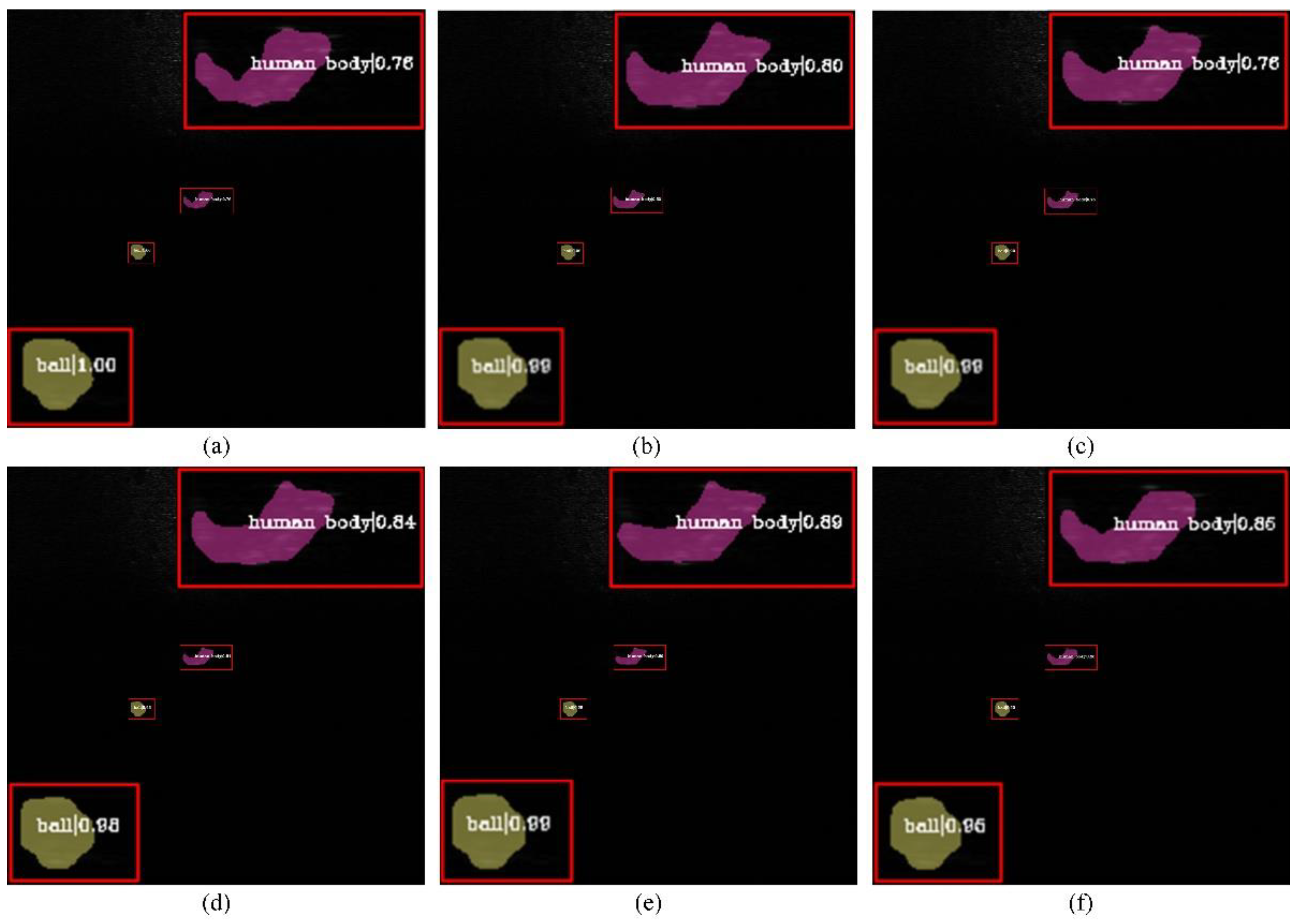
| Model | Position of GF-PSA | Value of n | mAP0.5:0.95 | mAP0.5 | mAP0.75 | AR | FPS |
|---|---|---|---|---|---|---|---|
| a | Between ResNet and FPN | n = 2 | 34.2% | 70.6% | 32.0% | 38.2% | 12.12 |
| b | n = 4 | 36.7% | 74.1% | 32.8% | 40.3% | 12.33 | |
| c | n = 8 | 34.0% | 67.5% | 32.3% | 37.5% | 12.27 | |
| d | After FPN | n = 2 | 35.1% | 70.9% | 33.0% | 39.7% | 12.11 |
| e | n = 4 | 36.1% | 74.9% | 32.2% | 39.8% | 12.14 | |
| f | n = 8 | 31.8% | 67.9% | 26.2% | 35.7% | 12.39 |
| Model | mAP0.5:0.95 | mAP0.5 | mAP0.75 | AR | FPS |
|---|---|---|---|---|---|
| Mask R-CNN | 33.7% | 71.0% | 27.6% | 36.4% | 4.6 |
| YOLACT | 32.8% | 66.8% | 15.3% | 33.5% | 10.1 |
| Polar Mask | 31.9% | 67.6% | 14.2% | 33.2% | 9.3 |
| SOLO v2 | 34.7% | 70.4% | 29.7% | 38.5% | 12.11 |
| Attentive SOLO | 36.7% | 74.1% | 32.8% | 40.3% | 12.33 |
| Attention Mechanism | mAP0.5:0.95 | mAP0.5 | mAP0.75 | AR | FPS |
|---|---|---|---|---|---|
| SENet | 34.1% | 70.6% | 33.9% | 37.8% | 11.65 |
| DANet | 34.3% | 69.0% | 32.0% | 37.5% | 12.14 |
| CBAM | 31.1% | 63.8% | 32.7% | 35.0% | 12.39 |
| PSA | 34.9% | 69.6% | 32.3% | 39.2% | 12.22 |
| GF-PSA | 36.7% | 74.1% | 32.8% | 40.3% | 12.33 |
Publisher’s Note: MDPI stays neutral with regard to jurisdictional claims in published maps and institutional affiliations. |
© 2022 by the authors. Licensee MDPI, Basel, Switzerland. This article is an open access article distributed under the terms and conditions of the Creative Commons Attribution (CC BY) license (https://creativecommons.org/licenses/by/4.0/).
Share and Cite
Huang, H.; Zuo, Z.; Sun, B.; Wu, P.; Zhang, J. Attentive SOLO for Sonar Target Segmentation. Electronics 2022, 11, 2904. https://doi.org/10.3390/electronics11182904
Huang H, Zuo Z, Sun B, Wu P, Zhang J. Attentive SOLO for Sonar Target Segmentation. Electronics. 2022; 11(18):2904. https://doi.org/10.3390/electronics11182904
Chicago/Turabian StyleHuang, Honghe, Zhen Zuo, Bei Sun, Peng Wu, and Jiaju Zhang. 2022. "Attentive SOLO for Sonar Target Segmentation" Electronics 11, no. 18: 2904. https://doi.org/10.3390/electronics11182904