1. Introduction
Many applications, from research to industry, including many aspects of our daily lives, currently benefit from advances in deep learning (DL) techniques.
We are living in a data deluge: petabytes of data are produced worldwide every year. This is exactly the ideal terrain for the growth of a variety of techniques capable of extracting patterns or, more generally, extracting knowledge from data. The paradigm of data science springs from the idea of extracting knowledge from this enormous set of data patterns [
1]. However, scientific progress has historically been associated with the process of generating and validating theories that should be subjected to observations. This opposite paradigm has been known as the scientific method since the 17th century. In the era of Big Data, samples are continuously collected without any specific theoretical basis. On the one hand, this can lead to the creation of new frameworks for knowledge discovery in many applications [
2,
3], but on the other hand, it can also lead to systematic neglect of scientific theories. Indeed, the success of black-box applications of data science can be seen as “the end of theory” [
4] since they generally do not require scientific assumptions.
Between these two extremes, new strategies have been developed in recent years that take advantage of both sides. All techniques that attempt to incorporate theory-based (e.g., laws of physics) domain knowledge into otherwise blind, data-driven models can be grouped under the paradigm of Theory-Guided Data Science (TGDS) [
5]. This new approach aims to enrich the classical integration of prior knowledge into machine learning. In the past, feature engineering and labeling were applied to make the models aware of the real-world constraints of the solution before inferring them. New approaches include the addition of logical rules [
6], algebraic [
7,
8] or differential [
9] equations as constraints on the loss functions of neural networks.
The need for models that take prior knowledge into account is paramount in all contexts that suffer from a lack of data. Moreover, scientific problems generally exhibit non-stationary patterns that change dynamically over time. Purely data-driven solutions therefore might fail to capture the true meaning of past measurements, leading to unreliable conclusions.
In recent years, some surveys [
5,
10,
11] have tried to collect the different techniques that combine theory-guided and data-driven modeling. The main difficulty is that any state-of-the-art solution is a priori very domain specific. Therefore, it is very difficult to compare the contribution that a selected strategy can make in solving a particular problem. To the best of out knowledge, we found no other works in literature addressing the task of comparing the different ways of implementing theory-injection techniques to multiple use cases. Then, the contribution of this paper is to perform such an experimental comparison by highlighting the key building blocks offered by different state-of-the-art solutions in three popular application contexts. Thus, the contribution is twofold:
experimentally replicating different state-of-the-art algorithms applied in three scientific contexts in a comparable manner;
providing a unified formalism that groups the theory-driven elements proposed in the prior art and their corresponding experimental evaluation to measure their contribution to the final model performance when varying the cardinality of the datasets.
The works analyzed in this paper have been chosen among the most representative found in the cited surveys for which both data and code are available.
The paper is organized as follows.
Section 2 presents the related work from which the solutions were selected to be compared experimentally.
Section 3 describes the selected solutions and highlights the differences in context and strategies used.
Section 4 shows the experimental results of the comparative analysis, measuring the impact of each theory-guided strategy on the overall performance of the model. Finally,
Section 5 draws conclusions and presents future work.
2. Related Works
The Theory-Guided Data Science (TGDS) [
5] paradigm has been successfully applied in various scientific domains, from climate science [
12,
13], to cyberphysical systems [
14], turbulence modeling [
15], material discovery [
16,
17], biological sciences [
18], quantum chemistry [
19], and hydrology [
8].
Von Rueden et al. [
10] categorized each approach according to (i) the source of the integrated knowledge, (ii) the representation of the knowledge, and (iii) its integration, i.e., where it is integrated into the learning pipeline.
2.1. Knowledge Source
The Source of the knowledge and whether it is formalized into a theoretical set of equations or rules can differentiate the kind of source in one of the following cases.
2.1.1. Scientific Knowledge
Typically formalized and validated through scientific experiments and/or analytical demonstrations. In this category, all subjects of science, technology, engineering, and mathematics can be considered.
2.1.2. World Knowledge
General information from everyday life, without formal validation, can be considered an important element in enriching the learning procedure. This kind of knowledge is generally more intuitive and refers to human reasoning on the perceived world, for instance, the fact that a cat has two ears and can meow. Within this class, we can also consider linguistics, with syntax and semantics as examples.
2.1.3. Expert Knowledge
Still not necessarily formalized, expert knowledge is generally held by a restricted group of specialists. It can be formalized, for instance, by human-machine interfaces and validated through a comparison with a group of experienced people.
2.2. Knowledge Representation
The Knowledge Representation category effectively corresponds to the formalized element of the prior information. Depending on the knowledge available for each specific task, different representations can be adopted. The most widespread alternatives, and the more interesting for this discussion, are briefly reported in the following.
2.2.1. Equations
Since differential equations or algebraic equations are involved, the final solution could follow a partially known behavior or be subject to some constraints that can be formalized in equations. Constraints are generally associated with algebraic equations or inequalities. Notable examples are the energy-mass equivalence (i.e.,
) or the mass invariance reflected in the Minkowski metric, which has been integrated, for example, by a Lorentz layer in [
20]. With respect to inequalities, final or intermediate solutions may have some physical upper or lower bounds (e.g., the velocity of a body is always less than the speed of light). This scenario is analyzed in [
21], where the authors explore methods for incorporating priors such as bounds and monotonicity constraints into learning processes. Analogous considerations can be made for differential equations that govern the dynamic behavior of state variables, inputs, and outputs. This background is sometimes known but may not be feasible, partially known but not fully representative of the real solution, or completely unknown [
22]. For these scenarios, machine learning algorithms can be applied to solve differential equations, as in [
9], to learn the residual dynamics with known prior assumptions about the behavior of the solution, as in [
23], or finally to learn the spatiotemporal dynamics itself, as in [
24].
2.2.2. Simulation Results
Many physical systems can be modeled with simulators, which typically solve a mathematical model with variable precision. These results can be added together with the input data, eventually allowing the DL model to find the corrective terms to be added [
8].
2.2.3. Domain-Specific Invariances
Input data might have a peculiar invariance due to their structure, i.e., images to be classified can preserve some properties even with translations or rotations. Other kinds of data can be permutationally invariant or even time-invariant, or subject to periodicity. For each of these cases, some particular model architectures can better express these features [
25].
2.3. Knowledge Integration
The integration of knowledge into machine learning algorithms can occur either at the beginning of the pipeline, e.g., within the training dataset, or in the middle, in defining tailored architectures for learning strategies, or at the end, in driving model results.
The classic approach to embedding prior information into the data is feature engineering, where secondary data are generated from the sampled data to emphasize something that is already known in the specific domain. A well-known alternative is to add synthetic information obtained from simulated data, as in [
8] so that a final algorithm finds the residuals of such approximated solutions.
Prior information can then be introduced to constrain the learning procedure by adding a physically oriented loss function to the normal supervised functions. This general strategy can be summarized as follows [
11]:
where
is the measure of the supervised error (e.g., MSE, cross-entropy),
R is an eventual additional regularization term to limit the complexity of the model, and
is the theory-guided contribution. Finally,
and
are real-valued coefficients that can be used to weight the different contributions of the loss function. The last term can either incorporate algebraic, differential, or logical equations. In this scenario, the work of Willard et al. in [
11], when predicting the lake temperature over the variation of the depth, introduces a penalty for predictions leading to water density not respecting the theory-bounded increase with depth.
Beucler et al. [
26] instead enforced conservation laws in the context of climate modeling. Starting from these constraints, they apply them both as soft constraints in the loss function and as hard constraints by reducing the cardinality of the prediction of optimizable neural networks and computing the residual ones through fixed layers. An analogous idea applied to the AC optimal power flow is found in [
27].
A more sophisticated strategy for incorporating physical information into DL models can be conducted in the design of the model architectures themselves or, more generally, in the hypothesis set [
10]. When addressing tasks in which some intermediate variables are known to be relevant in the evaluation of the solution, a known approach is to give a physical value to some output neurons, e.g., by means of a loss function enforcing them to be equal to those variables [
19], or by using models pretrained on an intermediate task [
28]. From another point of view, DL architectures can be designed to naturally express relational inductive biases [
25] even before the training procedure. In this sense, convolutional layers are inherently suited for dealing with spatial invariants on images, while recurrent layers can track sequential features, such as time series. The component of DL, capable of applying this reasoning to arbitrary relational structures, is the Graph Neural Network (GNN). Graph layers can be the CNN’s counterpart to graph-structured data [
29] or even improve representation over knowledge graphs in image processing or natural language processing [
30].
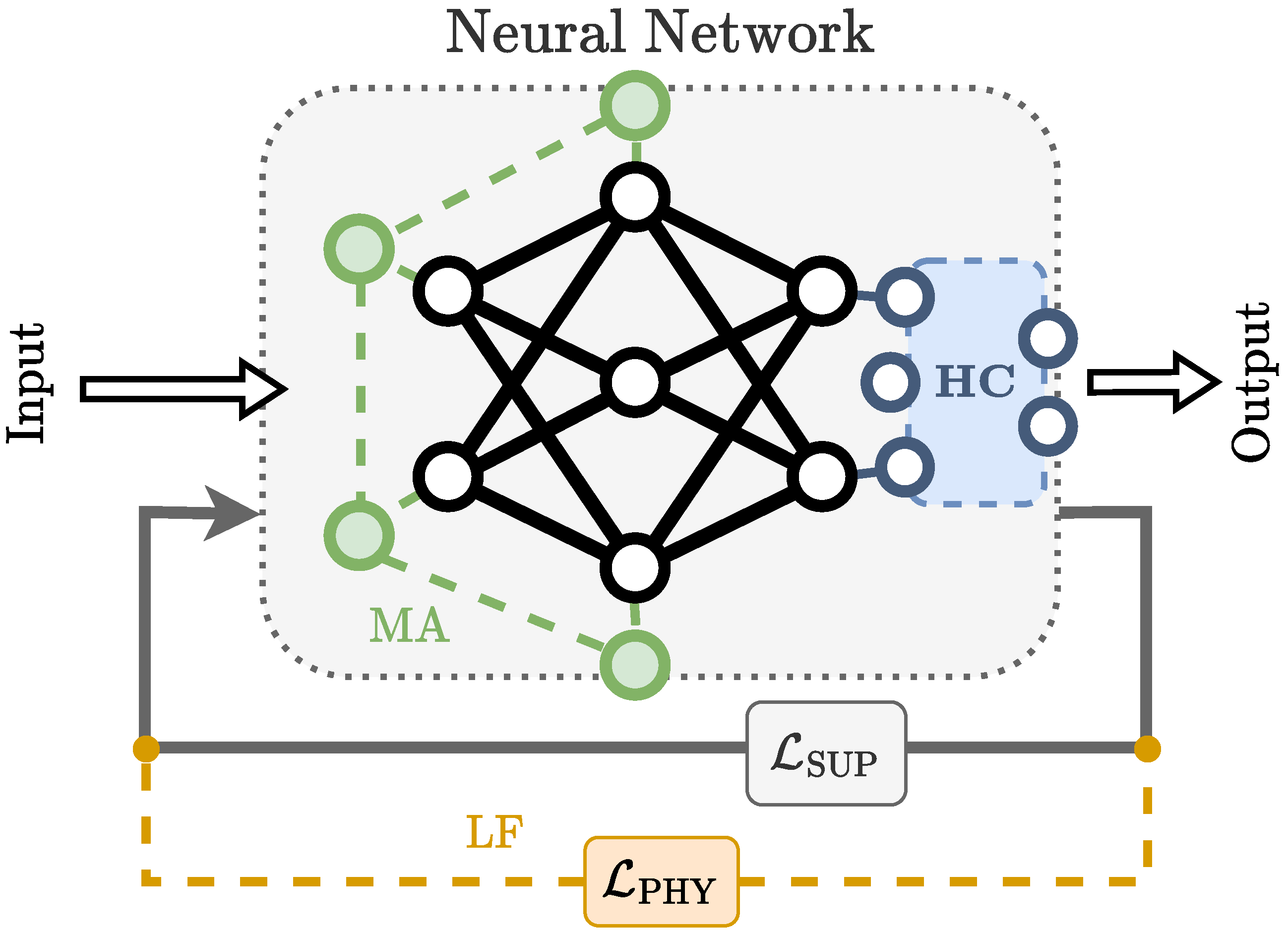
In the context of TGDS, we have selected for this experimental comparison the best papers that provide both code and datasets and are representative of the above strategies. They are listed below:
enforcing domain-specific constraints within the loss function (LF);
reducing the network output space in order to make the solution exactly fulfill the known hard constraints (HC);
incorporating the semantics of the problem to build a use-case specific model architecture in order to express the prior knowledge (MA).
These theory-guided building blocks are summarized in
Figure 1. In the next part of the section, we will show the analyzed works both highlighting the {source, representation, integration} triad and adopted building blocks.
3. Datasets and Methods
For each of the proposed strategies, we experimentally compare the state of the art in two application contexts, each defined by a specific dataset whose main characteristics, e.g., cardinality and size, are listed in
Table 1. The last row of the table refers to a graph dataset. Then, the cardinality and attribute dimension are specified for both vertices (here the product of static graph vertices and time samples) and edges.
3.1. Lake Temperature
The first study concerns the problem of modeling water temperature in a lake as a function of depth and weather conditions. We selected two papers by Daw et al. who first presented the Physics-Guided Neural Network (PGNN) [
8] and later addressed the same task with a recurrent neural network called Physics-Guided Architecture (PGA-LSTM from now on) [
31]. We compared the proposed architectures with the same dataset provided in [
31], while previous works were conducted with different datasets. The available data are a collection of weather measurements taken at Lake Mendota in Wisconsin, USA, between April 2009 and December 2017. Additional information is provided by simulated predictions of temperature.
PGNN consists of a multilayer perceptron (MLP) trained with a loss function with a physical term following the approach of Equation (
1). Such a loss formalizes the fact that water density increases monotonically with depth. Given the known analytical relationship between density
and temperature
t, the difference between successive densities (i.e., from depth
i to
), which are functions of the network predictions, must be negative to be consistent with this property. This led to the following physical loss:
In Equation (
2), ReLU function is applied to all density differences to consider only the contributions of the positive ones.
We can classify the PGNN algorithm according to the criteria of source, representation, and integration as follows: Source is scientific knowledge, representation is equations and simulation results, and integration is achieved by enriching training data and constraints in the learning procedure. The physical injection is performed here according to the LF strategy.
The same physical information, but with a different strategy, is introduced in the PGA-LSTM approach. Its architecture consists of an LSTM-based autoencoder that extracts temporal features from the input data and exploits repetition in the temporal dimension. The output of this first mesh is then appended and passed through a second recurrent mesh, which now operates in the depth dimension and is specifically designed to preserve the monotonicity of density over depth. This was accomplished by creating an additional recurrent link between density within the base LSTM architecture, which is enforced as a physical intermediate in a loss function that penalizes the mean square error between ground truth and the predicted value of temperature and density:
The architecture PGA-LSTM has the same knowledge source as the PGNN, but represents the knowledge through spatial and temporal invariances instead of equations, and integrates the knowledge into the model architecture itself. Therefore, we classify PGA-LSTM as an example of the MA strategy.
3.2. Convective Movements in Climate Modeling
The second experimental comparison context is the application of neural networks to climate modeling, as presented in [
26]. The goal of the network is to predict the rate at which heat and water are redistributed due to convective motions. The local climate is described by a set of over 300 variables that relate to thermodynamic properties over different elevation profiles as well as large-scale, non-elevation conditions. The goal of the network is then to predict the associated time trends of convection and additional variables from the system conservation laws. The total data are the simulated climate for 2 years using a parameterized atmospheric model [
32]. Among the many variables, the authors highlighted 4 conservation variables, namely column integrated energy, mass, longwave radiation, and shortwave radiation. These physical laws are translated into equations relating to input and output. Since they are derived as linear relationships, they can be substituted into a coefficient matrix
that yields zero when multiplied by the vector of inputs and outputs such that:
These constraints are then added either as soft constraints, i.e., the squared norm of as an additional loss function term, leading to an approach called LCNet; or as hard constraints, producing an ACnet. The latter strategy is performed by developing an MLP with trainable parameters and a number of initial features equal to the cardinality of minus the number of constraints, concatenating the other features obtained in a deterministic way.
For both LCNet and ACNet, the information is provided by scientific knowledge as the source and equations as the representation. Instead, we can determine the integration by the loss function in the first case and by hypotesis set in the second case. For this reason, the two strategies are compared as representatives of the solutions applying the LF and the HC, respectively.
3.3. Climate Prediction
The third work in our comparison consists of a GNN architecture applied to the task of climate prediction [
23]. The authors use the graph network component to predict the state at time
, assuming it is the same at time
t, to incorporate dynamical physics into this formalism. They extend the natural definitions of temporal and spatial derivatives to the inputs/outputs of the network and within the network itself, through nodes connected by undirected edges. Therefore, the differential equations underlying the nature of the problem are written in terms of these elements, and the process is then repeated recursively to mimic the evolution of the system. The basic assumption is that the entire physical system is much more complex than known physical knowledge. Therefore, the model should be able to extract patterns from the data to express this complexity while following the known components of the dynamics. Wind vectors and pressure most likely follow diffusive properties, even though this is not the only component of motion. This physical information is then provided by a physical loss term that expresses a diffusion penalty using the proposed GNN formalism. One defined the way of calculating the velocities
on the graph nodes, such a loss function term become
where
is a fixed coefficient adjusting the diffusivity of the latent physics quantities.
Climate observations were collected over 16 days in the Southern California region. Each vertex of the graph is a patch of the entire region and is connected to adjacent vertices by an edge. The vertices are expressed by 10 climate observations, while a static edge attribute was generated to track the land use of the patches that the edge connects. The final output of the network is then a temperature value for each node of the graph, obtained with an MLP decoder applied to the GNN block, to which the monitored loss is applied. In our experimental comparison, we analyze the average mean square temperature error output by the network after 10 steps of predicted wheat configurations.
We can classify this last TGDS approach as both LS and MA, since it has a scientific knowledge source represented with physical equations and domain invariants, and is integrated into both the loss function and the model architecture.
A summary of the knowledge source, representation, and integration for each of the approaches analyzed can be found in
Table 2.
4. Experimental Results
Since the main contribution of a theory-guided algorithm is its ability to obtain a reliable and physically consistent solution with a smaller amount of data, we evaluated all strategies experimentally by measuring their predictive power with variations in the size of the training data set. Each model was trained with a subset of the data, starting with the first timestamp. The test data set, on the other hand, was set as a separate subset. In order to obtain quantitative statistics on the results and their significance for comparison, the entire process was repeated 10 times for each experiment, with an experiment being identified by the tuple {use case, DL model, training-set percentage}. The results are then evaluated both in terms of average value and standard deviation.
A limitation of the current work is due to the seasonal effect of the start date: different algorithms may have different performance when selecting only a portion of the training set in a specific period of the year, with respect to another period. We plan to address this issue in future works. Currently, all comparisons were made under the assumption that the potential benefits of choosing different periods for training are common to all models.
4.1. Lake Temperature
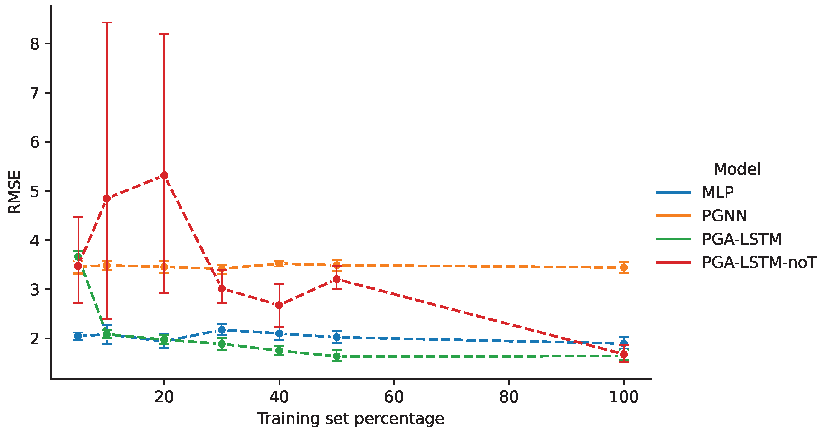
In
Figure 2, we compare the performance of the PGNN algorithm, its counterpart without the physical loss function (denoted MLP), and the algorithm PGA-LSTM on different training sets, alongside an additional experiment for PGA-LSTM without the temporal features extracted by the encoder (denoted PGA-LSTM -noT). The first notable observation is that the PGNN physical loss function does not contribute beneficially to any subset of the training set. On the other hand, the simple MLP achieves a valuable performance compared to other models by being the second best performing model after PGA-LSTM and is even tied for small percentages of the training set (10–20%). This suggests that the theory-based contribution may be limited for this simple problem. On the other hand, using the encoder to extract temporal features in PGA-LSTM contributes greatly to improving the results over PGA-LSTM -noT, especially for small training sets.
4.2. Convective Movements in Climate Modeling
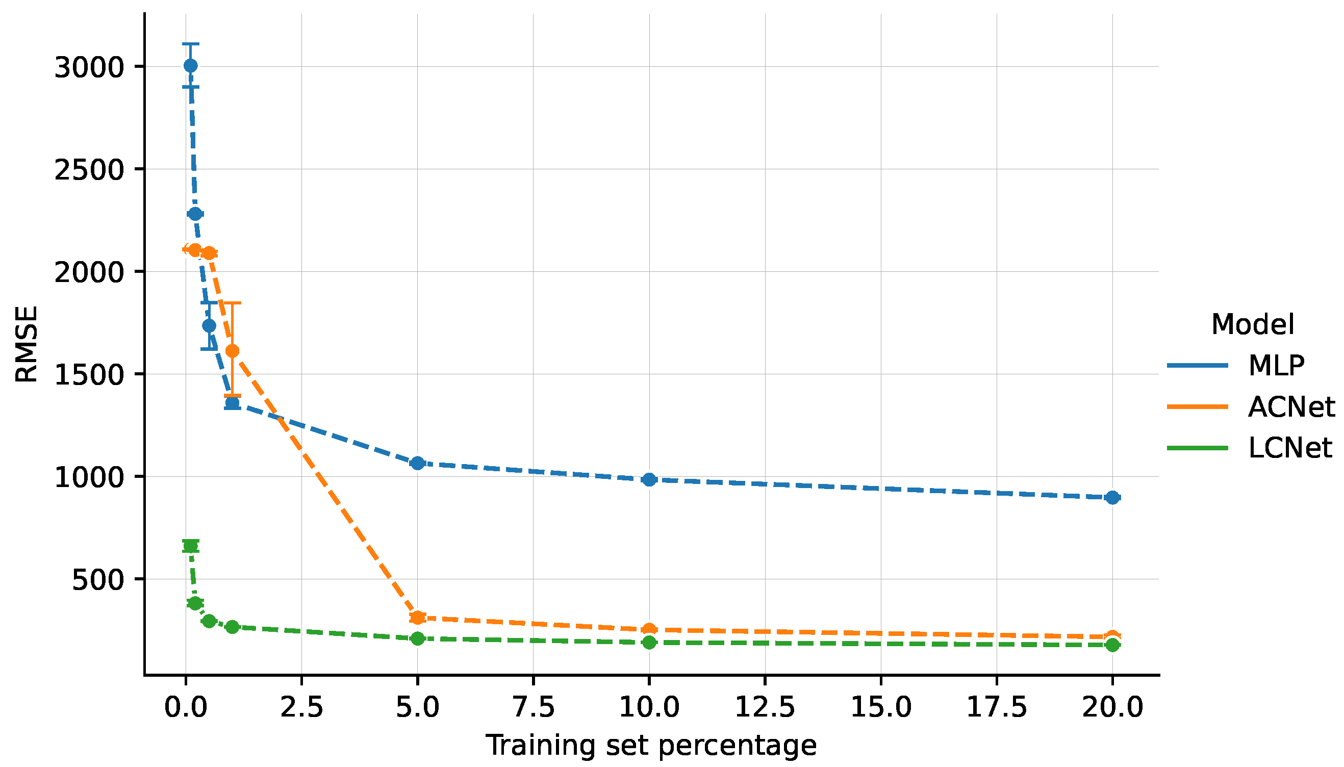
In
Figure 3, we compare a purely data-driven MLP architecture and the two theory-guided solutions LCNet and ACNet. Due to the much larger dimension of the data set (171 Gb compared to the few Mb of the other use cases), experiments are reported for 1–20% of the training set, with a clear asymptotic trend suggesting unsurprising behavior at larger sizes. With the largest training set (20%), the MLP achieves an RMSE of
, about four times higher than the two theory-guided approaches, with LCNet and ACNet at 176 and
, respectively.
The HC strategy (ACNet) strongly depends on the size of the training set: when the training set increases from 1 to 5% of the whole data set, the ACNet RMSE abruptly decreases from to . The MLP and LCNet also show the same trend for smaller training sets, below 1%. In this use case, the LCNet with the LF approach is the best performing solution, and its theory-driven injection leads to a large improvement over the purely data-driven MLP for all training sizes, and in particular, reaches a peak performance asymptote when trained on only 1% of the data set size. However, for such small training sizes (1%), the other theory-guided approach, ACNet, based on HC, is outperformed by the data-driven MLP, making the choice of the specific knowledge injection method a critical factor in TGDS solutions: it is not the case that all theory-guided approaches provide beneficial effects in all situations. We can interpret this evidence by assuming that ACNet is practically equivalent to MLP in terms of the learning part, but with a smaller number of weights to be trained. This leads to a relatively high RMSE when the information for training may be insufficient. On the other hand, LCNet also seems to offer advantages for smaller datasets. For a larger portion of the data set, LCNet shows a better profile for all experiments, but the difference with ACNet results is getting smaller. Considering that the latter network has the advantage of providing a full constraint match, this relatively small additional error could be negligible in all those situations where this second aspect is crucial. With respect to this analysis, we note that theoretical injection is definitely advantageous, but the choice of the element to apply may depend on the specific use case.
4.3. Climate Prediction
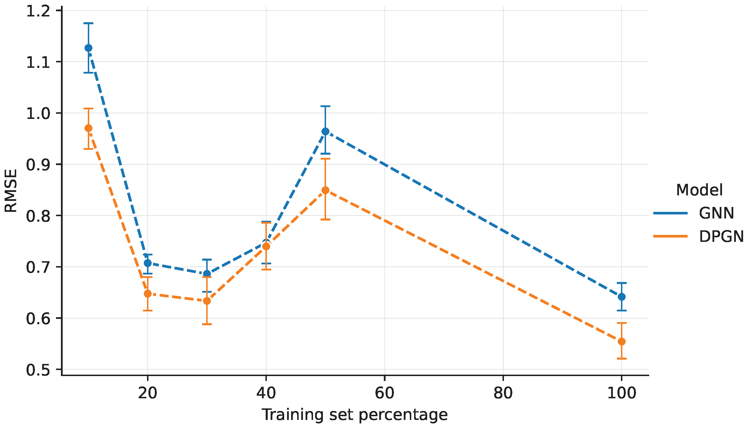
In
Figure 4, we compare the DPGN solution exploiting the building blocks LF+MA with its counterpart without the physical penalty in the loss function (GNN).
We know from the work of Seo et al. [
23] that a data-only MLP solution performs much worse compared to these two architectures: To avoid repetition, we refer readers to [
23] for details on this aspect. In our experiments, we observe that the DPGN outperforms the GNN in all training subsets, by a fairly constant margin. Both models show an unexpected behavior with a decreasing performance for the training set fraction between
and
. We hypothesize that this behavior can be explained by seasonal trends, which are not currently accounted for in our results.
5. Conclusions
The aim of the paper is to experimentally compare selected modern theory-guided approaches to evaluate the contribution of different techniques to the injection of a priori knowledge. We have divided knowledge injection into the building blocks of loss function (LF), hard constraints (HC), and model architecture (MA). Using three selected use cases for which the authors provided datasets and code, we compared the contribution of the different theory-guided injection techniques.
We evaluated the algorithms on variable portions of the datasets in order to test the effectiveness of the approaches in reaching valuable solutions with less data. The experimental comparison shows that not all the alternative methods always provide statistically significant improvements, e.g., for different training set sizes. However, it is globally evident that domain-injection methods can lead to benefits in performance with respect to traditional ones.
Although the results are preliminary in terms of the breadth of the field, we found that an architecture designed specifically for a physical phenomenon (MA) performs better on smaller data sets, with greater benefits for more complex problems. The more complex the physical problem, the greater the expected theory-guided improvement. However, theory-guided injection is not always advantageous for less complex problems, as in the lake temperature use case.
Forcing hard constraints (HC) has been shown to be effective in the convective motion use case, with comparable results compared to the soft loss function penalty approach. Nevertheless, the application is difficult because the strict equality conditions between input and output are not necessarily present in all use cases. In the literature [
26], the extension of this approach to inequality constraints, as upper bounds in parts of the solution, has been proposed. We plan to investigate this possibility or enforce restrictions even in situations where they are not strict, as in our third use case.
Finally, the domain-driven loss function (LF) seems to be the most promising. Although it does not give the best results in all comparisons when considered alone, it is easier to apply in most contexts. In fact, it is included in both proposed use cases of the paper and can possibly be integrated with other strategies.
In future work, we plan to extend the experimental comparison to new use cases and possibly provide more strategies for each use case, with the goal of identifying proposals for the most promising theory-driven approaches for different classes of scientific problems.
This preliminary experimental comparison is a promising step toward improving traditional data-driven algorithms, and the implications are not limited to scientific problems. In the future, we plan to conduct a systematic analysis of a larger number of use cases and establish a unified framework for knowing which is the best theory-guided way to formalize each aspect of human knowledge.
Author Contributions
Conceptualization, S.M. and D.A.; methodology, S.M.; software, S.M.; validation, S.M., D.A. and G.M.; formal analysis, S.M.; investigation, S.M.; resources, D.A.; data curation, S.M.; writing—original draft preparation, S.M.; writing—review and editing, S.M., D.A. and G.M.; visualization, S.M.; supervision, D.A.; project administration, D.A. All authors have read and agreed to the published version of the manuscript.
Funding
This research received no external funding.
Institutional Review Board Statement
Not applicable.
Informed Consent Statement
Not applicable.
Data Availability Statement
Acknowledgments
The research leading to these results has been partially supported by the SmartData@PoliTO center for Big Data and Machine Learning technologies.
Conflicts of Interest
The authors declare no conflict of interest.
References
- Dhar, V. Data science and prediction. Commun. ACM 2013, 56, 64–73. [Google Scholar] [CrossRef]
- Castelvecchi, D. Artificial intelligence called in to tackle LHC data deluge. Nature 2015, 528, 18–19. [Google Scholar] [CrossRef]
- Baldi, P.; Brunak, S. Bioinformatics: The Machine Learning Approach; MIT Press: Cambridge, MA, USA, 2001. [Google Scholar]
- Anderson, C. The end of theory: The data deluge makes the scientific method obsolete. Wired Mag. 2008, 16, 16-07. [Google Scholar]
- Karpatne, A.; Atluri, G.; Faghmous, J.; Steinbach, M.; Banerjee, A.; Ganguly, A.; Shekhar, S.; Samatova, N.; Kumar, V. Theory-guided Data Science: A New Paradigm for Scientific Discovery from Data. IEEE Trans. Knowl. Data Eng. 2017, 29, 2318–2331. [Google Scholar] [CrossRef]
- Diligenti, M.; Roychowdhury, S.; Gori, M. Integrating prior knowledge into deep learning. In Proceedings of the 2017 16th IEEE international conference on machine learning and applications (ICMLA), Cancun, Mexico, 18–21 December 2017; pp. 920–923. [Google Scholar]
- Stewart, R.; Ermon, S. Label-free supervision of neural networks with physics and domain knowledge. In Proceedings of the Thirty-First AAAI Conference on Artificial Intelligence, San Francisco, CA, USA, 4–9 February 2017. [Google Scholar]
- Daw, A.; Karpatne, A.; Watkins, W.; Read, J.; Kumar, V. Physics-guided neural networks (pgnn): An application in lake temperature modeling. arXiv 2017, arXiv:1710.11431. [Google Scholar]
- Raissi, M.; Perdikaris, P.; Karniadakis, G.E. Physics informed deep learning (part I): Data-driven solutions of nonlinear partial differential equations. arXiv 2017, arXiv:1711.10561. [Google Scholar]
- Von Rueden, L.; Mayer, S.; Beckh, K.; Georgiev, B.; Giesselbach, S.; Heese, R.; Kirsch, B.; Pfrommer, J.; Pick, A.; Ramamurthy, R.; et al. Informed Machine Learning—A Taxonomy and Survey of Integrating Knowledge into Learning Systems. arXiv 2021, arXiv:1903.12394. [Google Scholar] [CrossRef]
- Willard, J.; Jia, X.; Xu, S.; Steinbach, M.; Kumar, V. Integrating Scientific Knowledge with Machine Learning for Engineering and Environmental Systems. arXiv 2022, arXiv:2003.04919. [Google Scholar] [CrossRef]
- Faghmous, J.H.; Kumar, V. A big data guide to understanding climate change: The case for theory-guided data science. Big Data 2014, 2, 155–163. [Google Scholar] [CrossRef]
- O’Gorman, P.A.; Dwyer, J.G. Using machine learning to parameterize moist convection: Potential for modeling of climate, climate change, and extreme events. J. Adv. Model. Earth Syst. 2018, 10, 2548–2563. [Google Scholar] [CrossRef]
- Rai, R.; Sahu, C.K. Driven by Data or Derived Through Physics? A Review of Hybrid Physics Guided Machine Learning Techniques With Cyber-Physical System (CPS) Focus. IEEE Access 2020, 8, 71050–71073. [Google Scholar] [CrossRef]
- Mohan, A.T.; Gaitonde, D.V. A deep learning based approach to reduced order modeling for turbulent flow control using LSTM neural networks. arXiv 2018, arXiv:1804.09269. [Google Scholar]
- Cang, R.; Li, H.; Yao, H.; Jiao, Y.; Ren, Y. Improving direct physical properties prediction of heterogeneous materials from imaging data via convolutional neural network and a morphology-aware generative model. Comput. Mater. Sci. 2018, 150, 212–221. [Google Scholar] [CrossRef]
- Raccuglia, P.; Elbert, K.C.; Adler, P.D.; Falk, C.; Wenny, M.B.; Mollo, A.; Zeller, M.; Friedler, S.A.; Schrier, J.; Norquist, A.J. Machine-learning-assisted materials discovery using failed experiments. Nature 2016, 533, 73–76. [Google Scholar] [CrossRef]
- Peng, G.C.; Alber, M.; Buganza Tepole, A.; Cannon, W.R.; De, S.; Dura-Bernal, S.; Garikipati, K.; Karniadakis, G.; Lytton, W.W.; Perdikaris, P.; et al. Multiscale modeling meets machine learning: What can we learn? Arch. Comput. Methods Eng. 2021, 28, 1017–1037. [Google Scholar] [CrossRef]
- Muralidhar, N.; Bu, J.; Cao, Z.; He, L.; Ramakrishnan, N.; Tafti, D.; Karpatne, A. Phynet: Physics guided neural networks for particle drag force prediction in assembly. In Proceedings of the 2020 SIAM International Conference on Data Mining, Cincinnati, OH, USA, 7–9 May 2020; pp. 559–567. [Google Scholar]
- Butter, A.; Kasieczka, G.; Plehn, T.; Russell, M. Deep-learned top tagging with a Lorentz layer. SciPost Phys. 2018, 5, 28. [Google Scholar] [CrossRef]
- Muralidhar, N.; Islam, M.R.; Marwah, M.; Karpatne, A.; Ramakrishnan, N. Incorporating Prior Domain Knowledge into Deep Neural Networks. In Proceedings of the 2018 IEEE International Conference on Big Data (Big Data), Seattle, WA, USA, 10–13 December 2018; pp. 36–45. [Google Scholar] [CrossRef]
- Wang, R.; Yu, R. Physics-Guided Deep Learning for Dynamical Systems: A Survey. arXiv 2022, arXiv:2107.01272. [Google Scholar]
- Seo, S.; Liu, Y. Differentiable Physics-informed Graph Networks. arXiv 2019, arXiv:1902.02950. [Google Scholar]
- Kashinath, K.; Mustafa, M.; Albert, A.; Wu, J.; Jiang, C.; Esmaeilzadeh, S.; Azizzadenesheli, K.; Wang, R.; Chattopadhyay, A.; Singh, A.; et al. Physics-informed machine learning: Case studies for weather and climate modelling. Philos. Trans. R. Soc. A 2021, 379, 20200093. [Google Scholar] [CrossRef]
- Battaglia, P.W.; Hamrick, J.B.; Bapst, V.; Sanchez-Gonzalez, A.; Zambaldi, V.; Malinowski, M.; Tacchetti, A.; Raposo, D.; Santoro, A.; Faulkner, R.; et al. Relational inductive biases, deep learning, and graph networks. arXiv 2018, arXiv:1806.01261. [Google Scholar]
- Beucler, T.; Pritchard, M.; Rasp, S.; Ott, J.; Baldi, P.; Gentine, P. Enforcing Analytic Constraints in Neural Networks Emulating Physical Systems. Phys. Rev. Lett. 2021, 126, 098302. [Google Scholar] [CrossRef]
- Donti, P.L.; Rolnick, D.; Kolter, J.Z. DC3: A learning method for optimization with hard constraints. arXiv 2021, arXiv:2104.12225. [Google Scholar]
- Jia, X.; Zwart, J.; Sadler, J.; Appling, A.; Oliver, S.; Markstrom, S.; Willard, J.; Xu, S.; Steinbach, M.; Read, J.; et al. Physics-guided recurrent graph model for predicting flow and temperature in river networks. In Proceedings of the 2021 SIAM International Conference on Data Mining (SDM), Virtual Event, 29 April– 1 May 2021; pp. 612–620. [Google Scholar]
- Liang, X.; Hu, Z.; Zhang, H.; Lin, L.; Xing, E.P. Symbolic graph reasoning meets convolutions. In Proceedings of the NIPS’18: Proceedings of the 32nd International Conference on Neural Information Processing Systems, Red Hook, NY, USA, 3–8 December 2018; Volume 31. [Google Scholar]
- Peters, M.E.; Neumann, M.; Logan, R.L., IV; Schwartz, R.; Joshi, V.; Singh, S.; Smith, N.A. Knowledge enhanced contextual word representations. arXiv 2019, arXiv:1909.04164. [Google Scholar]
- Daw, A.; Thomas, R.Q.; Carey, C.C.; Read, J.S.; Appling, A.P.; Karpatne, A. Physics-Guided Architecture (PGA) of Neural Networks for Quantifying Uncertainty in Lake Temperature Modeling. arXiv 2019, arXiv:1911.02682. [Google Scholar]
- Khairoutdinov, M.F.; Randall, D.A. Cloud resolving modeling of the ARM summer 1997 IOP: Model formulation, results, uncertainties, and sensitivities. J. Atmos. Sci. 2003, 60, 607–625. [Google Scholar] [CrossRef]
| Publisher’s Note: MDPI stays neutral with regard to jurisdictional claims in published maps and institutional affiliations. |
© 2022 by the authors. Licensee MDPI, Basel, Switzerland. This article is an open access article distributed under the terms and conditions of the Creative Commons Attribution (CC BY) license (https://creativecommons.org/licenses/by/4.0/).


