1. Introduction
Topographic map data with 1:50,000 scale are one of the most basic geographic information data, which play a significant and strategic role in national economy and national defense construction [
1,
2]. With the rapid development of society, users have increasingly higher requirements for the current situation of topographic maps, and the updating of topographic maps [
3,
4] has become the primary and urgent work. The content of topographic maps mainly includes ground objects and the undulating form of terrain. Because the changes in terrain data are generally relatively small, the updated objects of topographic map mainly consist of ground objects.
Optical remote sensing imagery is one of the main data sources for updating ground objects in topographic maps. Ground object mapping mainly refers to the acquisition of object information in remote sensing imagery according to the corresponding scale graphic specification [
1]. At present, ground object mapping using remote sensing imagery is mainly completed manually, with high precision but low efficiency, making this kind of fashion tedious, expensive, and labor intensive, so it is difficult to meet the needs of rapid applications, such as land planning and automatic driving. According to official statistics [
5], it takes at least 40 days and 10 thousand RMB to produce 1:50,000 topographical map data. The number of global 1:50,000 topographical maps is about 400 thousand, and each update requires an investment of about 4 billion RMB.
With the launch of Zi-Yuan 3 (ZY-3) and Tian-Hui 1 (TH-1) stereo mapping satellites [
6,
7], China has the capability of measuring and updating 1:50,000 topographic maps with satellite remote sensing imagery. Among the ground feature elements, residential areas are one of the most important elements in topographic map content. A survey demonstrated that in most areas, the workload of extracting residential areas accounts for more than 60% of all the work of extracting ground features [
2]. Therefore, studying the automatic extraction method of residential areas for mapping applications is of considerable significance to improving the efficiency of mapping work.
With the development of this automatic extraction technology, many institutions around the world have developed digital mapping systems integrated with automatic technology for recognizing ground feature elements [
2]. For examples, both the eCognition [
8] of Definiens and the EasyFeature [
9] of Handleray have integrated the ground feature recognition technology. Specifically, this kind of method mainly includes two steps: extraction and post-processing.
Semantic segmentation [
10,
11] is a typical and an efficient technology to accomplish the extraction step, which indicates, dividing the image into pixel groups with specific semantics and recognizing each region’s category. In recent years, the development of deep learning techniques, such as convolution neural network (CNN), has injected new vitality into the study of semantic segmentation. However, due to the complexity of ground features and background in remote sensing imagery, the classification results of residential areas extracted by semantic segmentation method are usually not perfect, especially at residential area boundaries [
12], which are irregular contours. Consequently, these classification results cannot be directly employed in mapping applications. In addition, the post-processing technology is exploited to obtain the regularized object boundary contour. The popular operations used to identify the boundary of a raster dot group include smoothing, line segment fitting, denudation under complex constraints, and conditional random field (CRF) method, etc. In addition, there are also some methods using an end-to-end network to process the boundary of objects. The abovementioned innovative works focus on improving extraction accuracy but without consideration of the matching degree between the extraction results and the mapping requirement.
Obviously, the mapping method with two steps is cumbersome, and the post-processing step also greatly reduces the overall intelligence of the mapping method. End-to-end fashion can realize intelligent mapping without manual intervention. To promote the end-to-end mapping method, we present and introduce an optical satellite images dataset named RERB (Residential area Extraction with Regularized Boundary). To the best of the authors’ knowledge, there is no dataset released for the application of mapping residential area, which limits the research of end-to-end residential area regularization extraction. Compared to existing datasets, the contour of label image in RERB dataset consists of regular line segments. Given this point, it can facilitate the research for end-to-end training of residential area regularized extraction. Specifically, the public RERB dataset consists of 13,892 satellite images in 256 × 256 size, covering an area of more than 3640 square kilometers.
To summarize, our contributions are as follows:
- (1)
According to the specifications for cartographic symbols of 1:50,000 topographic map, our work summarizes the requirements of regular extraction in the residential area mapping application.
- (2)
We construct a residential area mapping dataset called RERB with regular contour labels based on TH-1 [
7] satellite images, which is the first dataset released for the residential feature mapping application. Furthermore, in order to measuring the compliance of the extraction results with the mapping requirements when using RERB dataset, we design a special evaluation index named CMI (contour matching index) based on contour matching. Extensive experiments demonstrate the superiority of RERB dataset.
- (3)
We sufficiently explore the contour constraint with regular contours in label images by integrating the contour cross-entropy constraint and the original loss function into an end-to-end network, which can significantly improve the regularization degree of extraction results for the mapping of residential areas.
The remainder of this paper is organized as follows:
Section 2 introduces the related works.
Section 3 presents the constructed RERB dataset in detail.
Section 4 details the experimental results along with in-depth analysis.
Section 5 finishes the paper with conclusions and our future perspective.
2. Related Works
In this section, we first describe the development of datasets for ground object extraction based on optical image and then introduce semantic segmentation methods. Finally, we introduce post-processing technology.
2.1. Datasets for Ground Object Extraction
Recently, with the advancement of deep learning technology, datasets have played an important part in ground object extraction. Any effective deep learning model is obtained by training with many original images and their corresponding labels. As shown in
Table 1, the widely used open-source datasets with optical image pixel level annotation include WHU [
13], LandCoverNet [
14], GID [
15], LoveDA [
16], SSD [
17], etc.
WHU dataset is released by Wuhan University, and it includes one land-cover category, namely, buildings. WHU dataset can be used to construct a building extraction model in a topographic map with a scale of 1:10,000 or larger and cannot be directly applied to residential area mapping in 1:50,000 scale topographic maps.
The Gaofen image dataset (GID) contains 150 high-quality GF-2 images from more than 60 cities in China, with a spatial resolution of 4 m. The size of each image is approximately 7200 × 6800 pixels, and it includes six land cover categories, namely, built-up, farmland, forest, meadow, water, and others, which represents all categories other than the former five categories. Similarly, LandCoverNet, LoveDA, and SSD are also constructed for land use and land cover (LULC) classification. If they are used for topographic mapping, post-processing steps still need to be added after model inference.
To study end-to-end regularized extraction technology of residential area, we propose the RERB dataset in this paper.
2.2. Semantic Segmentation
Semantic segmentation is a long-standing research topic that assigns a label to each pixel, known as pixel-level classification. In 2015, Long et al. [
18] proposed full connected networks (FCNs), whose excellent performance led researchers to change their understanding of semantic segmentation from regional clustering to pixel classification. At present, CNN-based methods have completely exceeded the segmentation accuracy of traditional methods. However, the training steps of FCNs are complex, and it is easy to lose pixel position information during up-sampling. After that, U-Net [
19], SegNet [
20], PSPNet [
21], the DeepLab family [
22,
23,
24], and FastFCN [
25] were developed. U-Net can effectively fuse multilevel feature maps, and small objects and large objects are processed by using shallow and deep information, respectively. U-Net is essentially a structure based on multiscale context and multilevel feature fusion. SegNet improves the segmentation accuracy by recording the position of pooled values in the original feature map and accurately mapping the relevant values to the corresponding positions in the up-sampling step. However, SegNet still fails to recover the object boundary very well. PSPNet integrates the multiscale background information with a pyramid pooling module. To obtain a larger receptive field, PSPNet improves the backbone network by using dilated convolutions [
26]. Furthermore, additional losses can provide the intermediate supervision information in PSPNet. The DeepLab series leads research on semantic segmentation. DeepLab v3+ [
24], which integrates more local information in low-level features and replaces the feature extractor with a more complex Xception network [
27], performs well on several public datasets. In addition, the atrous spatial pyramid pooling (ASPP) structure proposed by the DeepLab network has been widely employed in semantic segmentation research literature. FastFCN uses the joint pyramid up-sampling (JPU) module to improve the dilated convolution and obtains faster speed and higher accuracy.
Especially, semantic segmentation technology has been applied to remote sensing imagery and medical image [
28,
29] in recent years, which has greatly improved the research level of methods used to automatically extract ground feature elements. For example, Ying Sun et al. [
30] used optical images and light detection and ranging (LiDAR) data to construct multichannel input data and designed a convolution neural network (CNN) model with multiscale encoder–decoder architecture to achieve enhanced segmentation results. Cui et al. [
31] also improved the accuracy of building extraction by using the multiscale information of images. Y. Liu et al. [
32] jointly used LiDAR data and introduced a higher-order CRF to increase the accuracy of ground object segmentation. In addition, several researchers designed two-stage training approaches [
33], modified loss function [
34], self-attention modules [
35,
36], edge information [
37], or both self-attention and edge enhancement modules [
17] to fully exploit the context information of remote sensing imagery from a larger perspective.
2.3. Post-Processing Technology
The processing object of post-processing technology is the raster dot group, which is obtained by semantic segmentation. Traditional operations used to identify the boundary of a raster dot group include smoothing, line segment fitting, and denudation under complex constraints [
38,
39]. Most of these methods belong to the field of traditional image processing, and the degree of automation and intelligence is low.
Moreover, CRF [
40,
41,
42] methods are also widely used in post-processing of semantic segmentation results. Using CRF, the segmentation results can be corrected, especially at ground object borders. However, these CRF methods require the introduction of samples to the CRF control process, and this operation cause the CRF methods to lose their end-to-end characteristics. For mapping tasks based on automatic extraction technology, when the end-to-end characteristics are lost, the ground object mapping work must add an additional manual post-processing operation, which greatly reduces the overall intelligence of mapping tasks. Hence, new end-to-end methods must be introduced to solve this problem.
Ying Sun et al. [
43] first constructed multichannel input data using optical images and LiDAR data and then achieved a better result than SegNet by designing an end-to-end encoding–decoding structure. Meanwhile, the object boundary is strengthened. There are also some methods using an end-to-end network to process the boundary of objects, such as ACE2P [
44], Gated-SCNN [
45], and EaNet [
46]. The ACE2P model realizes end-to-end high-precision training by fully integrating the bottom characteristics, global contextual information, and edge details in the human body parsing task. Gated-SCNN is a double branch structure, in which the target shape information is embedded into the semantic segmentation network by a shape branch. Except for traditional semantic segmentation labels, image boundary labels are also needed in Gated-SCNN. To effectively separate confusing objects with sharp contours, EaNet is constructed based on a large kernel pyramid pooling (LKPP) module and a dice-based edge-aware loss function.
3. The RERB Dataset and Model Construction
This section first describes the contour requirements for mapping applications and then introduces the RERB dataset. Finally, we analyze the statistics for RERB dataset and describe the construction of a residential area regularized extraction model.
3.1. Contour Requirements for Mapping Applications
Different topographic maps are distinguished by scale and commonly used scales generally include 1:2000, 1:5000, 1:10,000, and 1:50,000. The 1:50,000 topographic map data are one of the most basic geographic information data. At present, ground object mapping using remote sensing imagery is mainly completed manually, with high precision but low efficiency, making this kind of fashion tedious, expensive, and labor intensive [
5]. As a result, it is very important to analyze the mapping requirements and build a mapping dataset to improve the intelligence of mapping work.
Topographic maps of different scales are constrained by corresponding graphic specifications, which mainly stipulates the symbols, annotations, and contour decoration of various ground objects and geomorphic elements represented on topographic maps, as well as the methods and basic requirements of using these symbols. This paper mainly focuses on 1:50,000 scale, and its corresponding current national standard [
1] was issued on 14 October 2017 and implemented on 1 May 2018.
Ground object mapping in surveying and mapping field mainly refers to the collection of the ground object information from remote sensing imagery according to the corresponding specification for cartographic symbols [
1].
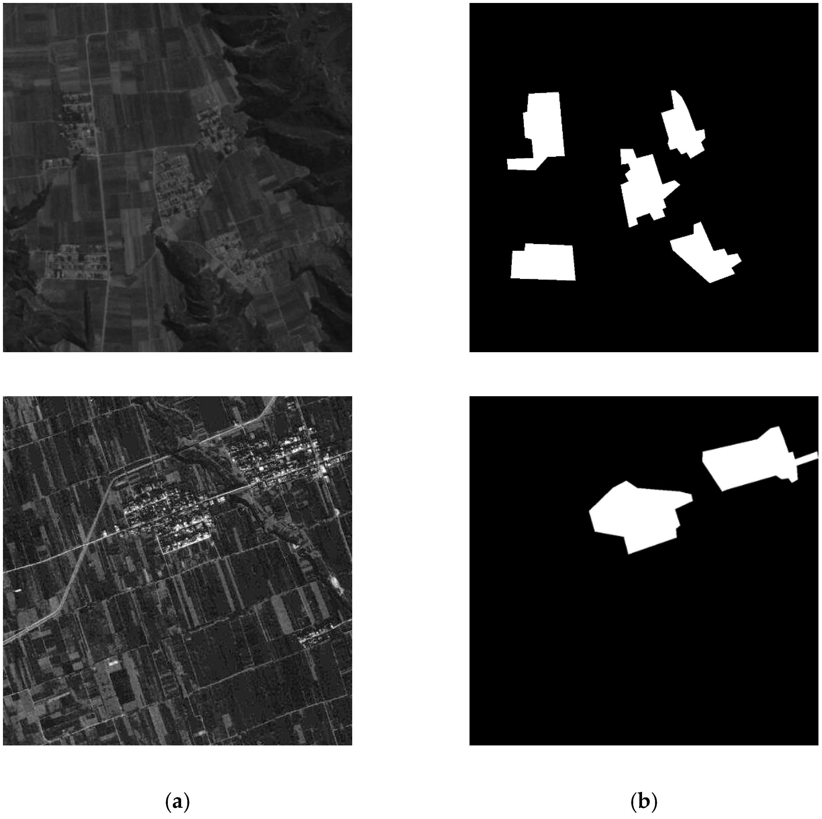
Figure 1 is an example of residential area extraction and mapping based on optical images.
Figure 1b is an illustration of a residential area in the 1:50,000 topographic map corresponding to the original image in
Figure 1a. Mapping is to obtain the contour of ground objects that meet the requirements of graphic specifications from remote sensing imagery.
Residential areas [
2] refer to houses that are contiguous to each other in cities, towns, and villages. There are obvious outer contours and primary and secondary streets in residential areas. The graphic specification [
1] stipulates that the convex and concave parts should be comprehensively represented when their length is less than 0.5–1 mm on the maps. In the 1:50,000 topographic map, 1 mm on the map represents the actual 50 m, and the length of 50 m is 25 pixels in the image with a resolution of 2 m. Therefore, the graphic specification requires that the convex and concave parts should be smoothed when their length is less than 12.5–25 pixels.
Figure 1c is a direct extraction result of residential areas based on semantic segmentation algorithms. The contour line is messy and has a high degree of border redundancy.
Figure 1b shows an illustration of the residential area layer in a topographic map, and it is a standard representation corresponding to the cartographic symbols used in topographic mapping. Its outer contour is multiple straight-line segments. The comparison indicated that the results of traditional semantic segmentation algorithms are different from the requirements of the cartographic symbols, and the contour of the extracted results must be regularized as much as possible.
To sum up, the extracted contour is required to be regular when images are used for residential area mapping. Each segment of extracted contour is generally a straight-line segment, which is relatively regular. Therefore, when building a dataset that supports the end-to-end regularization extraction of residential areas, it is necessary to ensure that the label image contour meets the regularization requirements.
3.2. Overview and Data Properties
In order to create RERB dataset, we collected 13,892 high-resolution TH-1 images [
7], and the size of each image is approximately 256 × 256 pixels.
Figure 2 shows the label visualization result in this dataset. The TH-1 satellite is the first stereo mapping transmission satellite in China, and its goal is to achieve topographic mapping at a 1:50,000 scale without using ground control points. It consists of a high-resolution camera with ground pixel size of 2 m and a multispectral camera with a ground pixel size of 10 m. Images with a spatial resolution of 2 m are applied in this dataset, and these images cover a geographical area of more than 3640 square kilometers.
The proportions of residential area and other land cover categories in RERB dataset are shown in
Table 2. It is obvious that the proportion of the residential area is lower than that of the other categories, which is consistent with the distribution of large-scale remote sensing imagery scenes.
The labels used for traditional semantic segmentation usually do not have regularization characteristics, as shown in
Figure 3b. This kind of label is assigned accurately according to the actual range of residential areas in the image [
42]. Different from semantic segmentation labels, according to the contour regularization requirements in mapping application, we need to ensure the labels of residential areas into a regular format.
In addition to the regularization requirements of contour line segments, special attention should also be paid to the treatment of the included angle between line segments when labeling. The main principles include small contour protrusion removal and small contour concave part filling. As shown in
Figure 4, using the interior of the patch as the reference direction, the contour protrusion and the concave part of the contour are defined when the angle between contour segments is too small (<45°) and excessively large (>90°), respectively. These situations will be corrected with blunt or right angles. For example, in
Figure 3b, there are small acute angles as shown in the red circles at the corner of residential areas. Therefore, as shown in
Figure 3c, we edit these angles by using a right angle or an obtuse angle in mapping application labels.
We split 85% of these images into the train set and leave the remaining 15% as the test set. As for annotation, RERB dataset provides pixel-level labels for two important categories, including background and residential area. They are labeled with black (0) and white (1).
We also analyze RERB dataset and find it has four properties: (1) Large-scale and high-resolution. As shown in
Table 1, RERB contains 13,892 high-quality satellite images acquired from different cities in China. It covers an area of more than 3640 square kilometers. (2) Well annotated and regular label contour. For each satellite image, we provide accurate pixel-wise mapping application labels for two categories (‘background’ and ‘residential’ area), which are annotated by a group of experts. (3) Rich background. The remote sensing mapping task is always faced with the diverse background samples (i.e., ground objects that are not of interest). The high-resolution and different scenes bring more rich details for the background samples. (4) Class imbalance. As shown in
Table 2, two categories have very different proportions, which lead to a class imbalance problem. This problem poses a special challenge for the regularization extraction of the residential areas task.
3.3. Statistics for RERB Dataset
Some statistics of the RERB dataset are analyzed in this section. The number of labeled pixels has been counted. As is shown in
Table 2 and
Figure 5a, the background class contains the most pixels with rich and diverse background samples, which cause special challenge for residential areas extraction.
For the spectral statistics (
Figure 5b), the background category has a lower mean value (color column) and standard deviation (vertical line). Because of the high-resolution images of TH-1 satellite are single channel, the values of red, green, and blue are same. As is shown in
Figure 5c, most of the residential areas have relatively small scales. Through calculation, the average size of the minimum 30% residential areas is about 479.71 pixels, and the average size of the maximum 30% residential areas is about 18,851 pixels. The multiscale residential areas require the models to have multiscale capture capabilities.
3.4. Construction of Residential Area Regularized Extraction Model
The common semantic segmentation network is generally a symmetric network with encoding–decoding structure [
19,
20]. The encoding operations mainly include convolution and pooling. Convolution is used to extract high-dimensional features of the input image, and pooling is used to make the image smaller. The decoding operations mainly include deconvolution and up-sampling. Deconvolution makes the features of the image reappear after classification, and up-sampling can restore the original size of the image. Finally, the classification results of each pixel are output. In terms of loss function, cross-entropy [
46] has been the most widely used loss function in semantic segmentations of images.
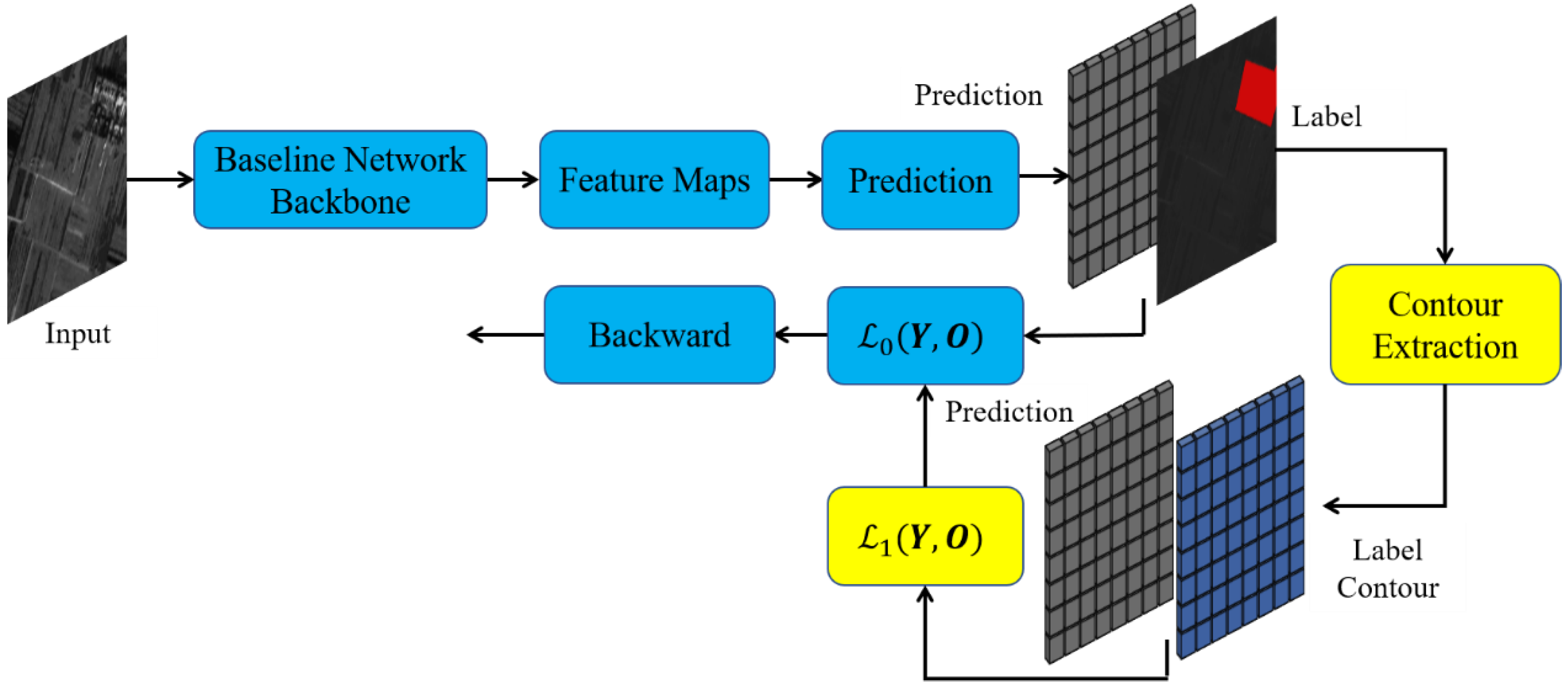
In order to test the effectiveness of the RERB dataset, we designed an end-to-end regularized extraction network by analyzing the regularization characteristics of label contour and the constraints of loss function.
As shown in
Figure 6, compared with the traditional semantic segmentation network in
Figure 7, our method extracts the contour of the label image first, and realizes regularization extraction by adding the cross-entropy constraint of the label contour image and model prediction image to the original loss function. The baseline method chosen in this article can be any semantic segmentation network, such as U-Net [
19] or DeepLab v3+ [
24].
The cross-entropy loss function can make the predicted image learned from the training data similar to the real label image. Considering that the label image contour of RERB dataset already has good, regularized contour characteristics, we first extract the contour of label image and then constrain the contour regularization degree of the network prediction image by calculating the cross-entropy loss between the label contour image and the network prediction image, as shown in Equation (1):
where
denotes the label image,
represents the image size,
is the network inference result image, which has the same size as image
.
and
represent the cross-entropy loss function and the contour extraction function, respectively.
represents the degree of inconsistency between the contours of the two images. Through the calculation and back propagation of
in the training process, the contour of the prediction image can be made more and more regular. The cross-entropy loss function is expressed as follows:
where
and
denotes the value at position
in the image
and
, respectively.
The contour of the label image can be extracted by the corrosion of a 3 × 3 structuring element. Corrosion is a commonly used morphological operation in an image processing file, and it can be expressed as follows:
In the above formula, the corrosion operation can remove the area contour in the image , and then the contour image can be obtained by subtracting the corroded image from the original image.
In the training stage, the Adam [
47] optimizer is adopted, and it is a first-order optimization algorithm. The best model can be obtained by minimizing joint loss function
, which is shown in the following formula:
where
is the original loss function of the baseline network, and the functions used in this paper include cross-entropy and Lovász [
48]. The existence of
can ensure the segmentation accuracy of the original semantic segmentation network.
and
are the two weights of loss functions, which are experimentally determined.
4. Experiment and Analysis
In this section, we carried out experimental verification and tested the effectiveness of the RERB dataset by using the model constructed in
Section 3 and
Section 4. We first introduced the evaluation metrics. Then, we performed an ablation study to determine some parameters. In the contrast experiment, the baseline networks were U-Net and DeepLab v3+. All experiments were carried out on a platform with an Intel Core (TM) i9 3.60 GHz CPU, 32 GB RAM, GeForce GTX 2080 GPU, and 11 GB video memory. These algorithms were implemented using PyTorch 1.0 and Python 3.7.
4.1. Design of Evaluation Metrics
The traditional semantic segmentation evaluation indexes, such as mean intersection over union (
mIoU) [
18], mainly evaluated the extraction accuracy in pixel units, which cannot reflect the regularization degree of contours as a whole. In detail, the calculation of
mIoU was based on the confusion matrix, as shown in
Table 3. There were
different classes in total, including backgrounds, where
was the number of pixels of class
predicted to belong to class
and
was the total number of pixels of class
.
Therefore,
mIoU is calculated as follows.
To quantitatively evaluate the regularization extraction results, a contour matching index (CMI) was designed to measure the performance of the algorithm in this paper. The specific steps of the CMI calculation are as follows.
- (1)
The contours of the model prediction image (
Figure 8b) and the label image (
Figure 8c) were extracted, and the results are shown in
Figure 8d,e;
- (2)
The distance transform of the contour of label image was computed, as shown in
Figure 8f;
- (3)
A contour matching value was obtained by matching the contour of the model prediction image (
Figure 8d) with the distance transformed image (
Figure 8f);
- (4)
The CMI value of this image was obtained by dividing the matched value by the number of pixels in the contour of the label image.
The critical factor of the distance transform [
49] was the definition of distance. In this paper, a block distance transform was adopted. The pixel value of the true contour point was 0 in the image after the distance transform was computed. The farther away from the true contour point, the larger the pixel value of the transformed image. Thus, the matching value can be obtained by calculating the sum of pixel values in the transformed image corresponding to the position of the contour points in the model prediction image. Since the contour image was a binary image that contained only the residential area point (pixel value 1) and the background point (pixel value 0), the matching values between
Figure 8d,f can be calculated as follows:
where
is the pixel coordinate,
and
are pixel values at
in
Figure 8d,f, respectively, and
represents the total number of contour points in label contour image
(
Figure 8e).
The value reflected the matching degree between the prediction result and the value image. The smaller the value was, the higher the matching degree. Furthermore, the average CMI of all images was used as the evaluation result when a whole test set was evaluated.
Considering that the background class occupied most of the image, we removed the background class in the calculation of mIoU to prevent it from affecting the evaluation of other ground features. Therefore, the evaluation indexes included the CMI and IoU of residential areas.
4.2. Parameters Settings and Ablation Study
4.2.1. Parameters Settings
In the experiment, we divided the training set and test set according to the ratio of 17:3. Finally, the training set and the test set contained approximately 13,611 image slices and 281 image slices, respectively. To verify the adaptability of the proposed method to different loss functions, Lovász was used for when the baseline network was U-Net, and cross-entropy was used for when the baseline network was DeepLab v3+. The number of ground feature elements was set as .
The polynomial learning rate policy was employed where the initial learning rate was multiplied by
after each iteration. The maximum number of training cycles was 100 epochs, and thus,
. The optimal model was determined by testing the model epoch by epoch during training. The weight decay coefficient was set to 0.0005. In terms of the optimization method, the Adam [
47] optimizer was used for training.
Batch size value had a great impact on model training and quality of results. Usually, we selected the maximum value according to the network parameters and the hardware configuration (mainly the video memory of GPU). In this paper, we carried out experiments with a batch size of 8, which was determined by model size and video memory. The selection principle was to make the video memory not overflow.
4.2.2. Ablation Study
In this section, we first studied the influence of the initial learning rate on the test set of the RERB dataset. To perform this ablation study, we adopted the semantic segmentation network and the metric mIoU. We evaluated the performance pertaining to the abovementioned parameters, as described in
Table 4.
The experiments specified in
Table 4 were conducted with training batch size = 8. As shown in
Table 4, the
mIoU peaked when the initial learning rate was 2 × 10
−5.
Next, we studied the influence of the weight on the test set of the RERB dataset. The cross-entropy loss between the label contour image and the network prediction image was inserted to the above semantic segmentation models. The metric CMI was adopted in these experiments.
The experiments specified in
Table 5 were conducted with training batch size = 8 and the initial learning rate 2 × 10
−5. As shown in
Table 5, the CMI index of the proposed method reached the minimum value when
.
4.3. Results and Analysis
We parameter tuned some parameters of U-Net, DeepLab v3+ and our proposed method, and the quantitative evaluation results on the test set of RERB dataset are shown in
Table 6.
The contrasting experimental results are shown in
Figure 9. As seen from
Table 6 and
Figure 9, the regularization level of residential area contours extracted by our proposed method had increased greatly, especially those areas marked by white circles. When the baseline network was U-Net, the IoU of residential areas decreased by 0.51%, but the CMI increased by 39.54%. Moreover, both the IoU of residential areas and the CMI increased by 0.63% and 25.5%, respectively, when the baseline network was DeepLab v3+.
Compared with the semantic segmentation dataset, the label image contour in RERB dataset had the regularization characteristic and provided additional information, so it could support the construction and training of end-to-end regularization extraction model of residential areas. The experimental results demonstrated the preponderance and practicability of the RERB dataset.
In terms of computational complexity, according to the model construction method in
Section 3 and
Section 4, the increased calculation amount of this method compared with the basic network mainly included label image edge extraction and contour cross-entropy loss calculation during training. The operations of contour extraction included a corrosion operation with 3 × 3 structuring element and a subtraction. Contour cross-entropy loss calculation included logarithmic calculation and accumulation, which was the same as the original cross-entropy function. Therefore, during the training phase, the computational complexity of the proposed method was slightly larger than that of the traditional semantic segmentation network. Consequently, the runtime of training and the optimal epoch number of our method were higher than those before model modification. In the case of test time, our proposed method was at the same level with traditional models.
5. Conclusions
For residential areas, the difference between semantic segmentation labels and mapping application labels limits the possibility of end-to-end regularization extraction training. In order to address this problem, we built a dataset named RERB (Residential area Extraction with Regularized Boundary) for the end-to-end regularization extraction of residential areas. To ensure the rationality of RERB dataset, we analyzed the contour representation requirements for residential area mapping according to the graphic specification of 1:50,000 topographic map, and then transformed it into the following annotation requirements: the contour of label image should be regular, and the included angle of contour line segments should be as right angle as possible. Based on these principles, we have completed the annotation of residential areas in 13,892 image patches based on TH-1 images. The size of each image is approximately 256 × 256 pixels. The RERB dataset encompasses four properties: (1) Large-scale and high-resolution; (2) well annotated and regular label contour; (3) rich background; and (4) class imbalance. In reality, high resolution, complex background, and category imbalance represent three challenges in residential area mapping. Finally, a residential area regularization extraction model is constructed with a contour cross-entropy constraint by using the regular contour label of a residential area. Experimental results showed that the proposed algorithm can improve the regularization degree of the extracted contour of residential areas while maintaining nearly the same extraction accuracy. This fully proves the effectiveness of RERB dataset. In the future, we will expand and improve the dataset of mapping residential area and conduct in-depth research on the end-to-end model for mapping.


