1. Introduction
Large amounts of data are now freely available. As a result, it is necessary to analyze these data in order to extract useful information and then create an algorithm based on that analysis. This can be accomplished via data mining and machine learning (ML). ML is a subset of artificial intelligence (AI) that creates algorithms based on data trends and previous data correlations. Bioinformatics, wireless communication networking, and image deconvolution are just a few of the areas that use machine learning [
1]. The ML algorithms extract information from data. These data are accustomed to learning. This is what ML is used for [
2].
Because 6G is a revolutionary wireless technology that is presently undergoing academic study, the primary promises of 6G in wireless communications are to spread ML benefits in wireless networks and to customers. 6G will also improve technical parameters, such as throughput, support for new high-demand apps, and radio-frequency-spectrum usage using ML techniques [
3,
4]. The ML techniques are used to enhance the QoS.
The rising number of users necessitates a higher bandwidth need for future fixed fifth generation (F5G) connectivity [
5]. Optical code division multiple access (OCDMA) can be considered a dominant technique for supporting future applications that require simultaneous transmission of information with high performance [
6,
7,
8,
9,
10] among many multiple access techniques, such as time division multiple access (TDMA) and wavelength division multiple access (WDMA). Because time-sharing transmission is essential in TDMA systems, each subcarrier’s capacity is limited. Furthermore, transmitting various services, such as audio and data would need time management, which will be difficult [
7]. Furthermore, due to the necessity for a high number of wavelengths for users, WDM systems are insufficient for large cardinality systems [
6].
The following are the contributions of this paper:
The Q-Factor, SNR, and BER are studied as the ML input predictors. The statistical validation of the ML input samples is performed using hypothesis testing.
The multicollinearity of the features is detected using Pearson correlation matrix and the VIF score for each feature.
The ML approach adopted for the classification of the following four classes {SPD: Groups A/D, SPD: Groups B/C, DD: Groups A/D, DD: Groups B/C}. The DT and RF are integrating the model as ML classifiers. The evaluation of both classifiers is performed using confusion matrices and ROC curves.
The paper is organized as follows.
Section 2 is concerned with the model used as the normalization, multicollinearity detection, and ML classifiers are introduced.
Section 3 shows the results of each process where the evaluation of the hypothesis testing, Pearson correlation, and VIF are revealed. ML results are evaluated using correlation matrices and ROC curves. In the end,
Section 4 presents the conclusion and future work.
2. Dataset Validation and Preprocessing
The coupling of a laser beam in an optical fiber causes losses due mainly to its noncircularity and to the Fresnel reflections created at the injection face of the fiber. These reflections, moreover, disturb the proper functioning of the laser. The impact of these reflections on the stability of the optical source is easily avoided in a free-space assembly by using inclined optical surfaces, which deflect the beam but do not reduce losses. The constant reduction of the space requirement in the interrogators leads to using fiber components. In this case, it is possible to reduce the Fresnel reflections significantly by applying an antireflection coating to the injection face of the fiber.
The intrinsic propagation losses in AR fibers are due to diffusion at the interfaces, leaks, and absorption of the material. However, the losses due to scattering are considered negligible for this type of fiber, given the small amount of surface area seen by the light propagating, compared with photonic band-gap fibers.
This section shows the dataset validation. The total dataset features are extracted from Optisystem version 19. The features are Q-factor, SNR, and BER. The data response has four different groups carrying two different quality of services (video and audio) at different data rates—1.25 Gbps and 2.5 Gbps. These groups are assigned with variable weight fixed right shift (VWFRS) code that applies to a spectral amplitude coding optical code division multiple access (SCA-OCDMA) system using two detections schemes: direct detection (DD) and single photodiode (SPD). These are groups are:
- (1)
Group A/D for video service at 1.25 Gbps and odd weight FRS code with SPD scheme.
- (2)
Group B/C for audio service at 1.25 Gbps and even weight FRS code with SPD scheme.
- (3)
Group A/D for video service at 2.5 Gbps and odd weight FRS code with DD scheme.
- (4)
Group B/C for audio service at 2.5 Gbps and even weight FRS code with DD scheme.
The total number of unique groups is four, where the groups are {SPD: A/D, SPD: B/C, DD: A/D, DD: B/C}. The number of data points is equiprobable for all such classes. The sample data taken are validated through hypothesis testing. The rest of the workflow procedures are data normalization, data visualization, and multicollinearity detection.
2.1. Hypothesis Testing
To determine if the outcome of a dataset is statistically significant, statistical hypothesis testing is carried out. The probability that the difference in conversion rates between a particular variation and the baseline is not the result of random chance is known as statistical significance. This is shown by the
p-value, which is the degree of marginal significance in a statistical hypothesis test and represents the likelihood that a particular event will occur. To assess if there is a significant difference between the means of the two groups, which may be connected in certain attributes, the
t-test is a common sort of inferential statistic [
11]. The two groups in this case are the population and the sample for Q-factor, SNR and BER. The null hypothesis (
) is that the average of the sample set is the same as the population set. On the other hand, the alternative hypothesis (
) is that both averages can be differentiated. The hypothesis can be denoted as:
where F represents the features and i = 1, 2, 3 which represents the Q-factor, SNR and BER. The
t-test reveals
p-value of 0.97, 0.98 and 0.98 for Q-factor, SNR and BER, respectively.
A p-value greater than 0.05 provides strong support for the null hypothesis, but is not statistically significant. As a result, there is no statistical significance, and the null hypothesis cannot be rejected. The population’s distribution matches that of the sample. As a result, the test demonstrates the predictor dataset’s reliability.
2.2. Z-Score Normalization
Due of the high variance and outliers in the data, ML models may perform poorly and be complicated [
12]. Hence, every data point
should be subjected to data normalization and can be denoted as [
12]:
where
and
are the average and standard deviation of each feature
j.
2.3. Multicollinearity Detection
The multicollinearity shows the dependence of multiple features on the output. The preliminary detection of the features that formulate the multicollinearity problem may avoid the use of unwanted features. The Pearson correlation matrix and the VIF factor are adopted to detect the multicollinearity of the input features impacting the output.
The Pearson correlation matrix shows correlations between features. Covariance can be used to describe the correlation coefficients mathematically [
13]:
This formula has a few variables, each of whose definitions are as follows: is defined as the mean value of the sum after multiplying between the corresponding elements in two sets of data; denotes the average value of the sample X; is the mean value of the sample Y; denotes the standard deviation of the sample X; is defined as the standard deviation of the sample Y; is the correlation coefficient between X and Y, that is Pearson correlation coefficient. Generally defined as follow: 0.8 1.0, means extremely strong correlation; 0.6 0.8, means strong correlation; 0.4 0.6, means moderate correlation; 0.2 0.4, means weak correlation; 0.0 0.2, means extremely weak correlation.
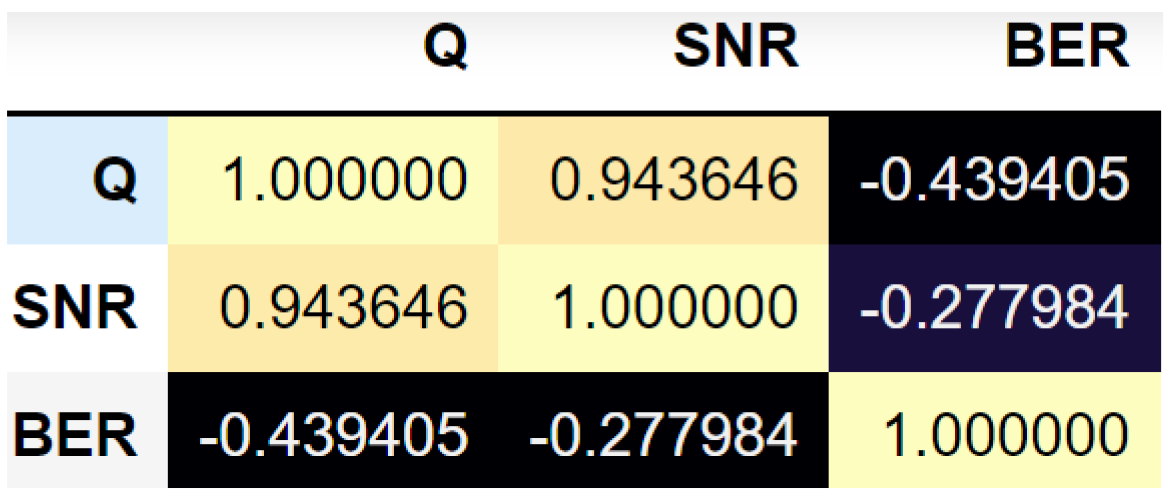
The resultant correlation matrix of the normalized features Q-factor, SNR and BER is represented in
Figure 1.
The brighter the cell represents the highly positive correlation. The diagonal represents the auto correlation coefficient (between the feature and itself). The correlation matrix shows that a highly strong positive correlation exists between the SNR and the Q-factor (denoted as Q) with a value of = 0.94. A moderate correlation exists between the BER and Q-factor. A negative weak correlation exists between the SNR and BER.
Moreover, the multicollinearity can be validated through
VIF using the method of [
14]
where
is the multiple
for the regression of a feature on the other covariates. The higher the
VIF, the lower the entropy of the information. The value of
VIF should not pass 10. If the value of
VIF is more than 10, then multicollinearity surely exists. The resultant
VIF for each feature is represented in
Table 1.
The Q-factor has the highest VIF with 4.49. The SNR and BER achieve 3.88 and 1.34, respectively.
2.4. Data Visualization
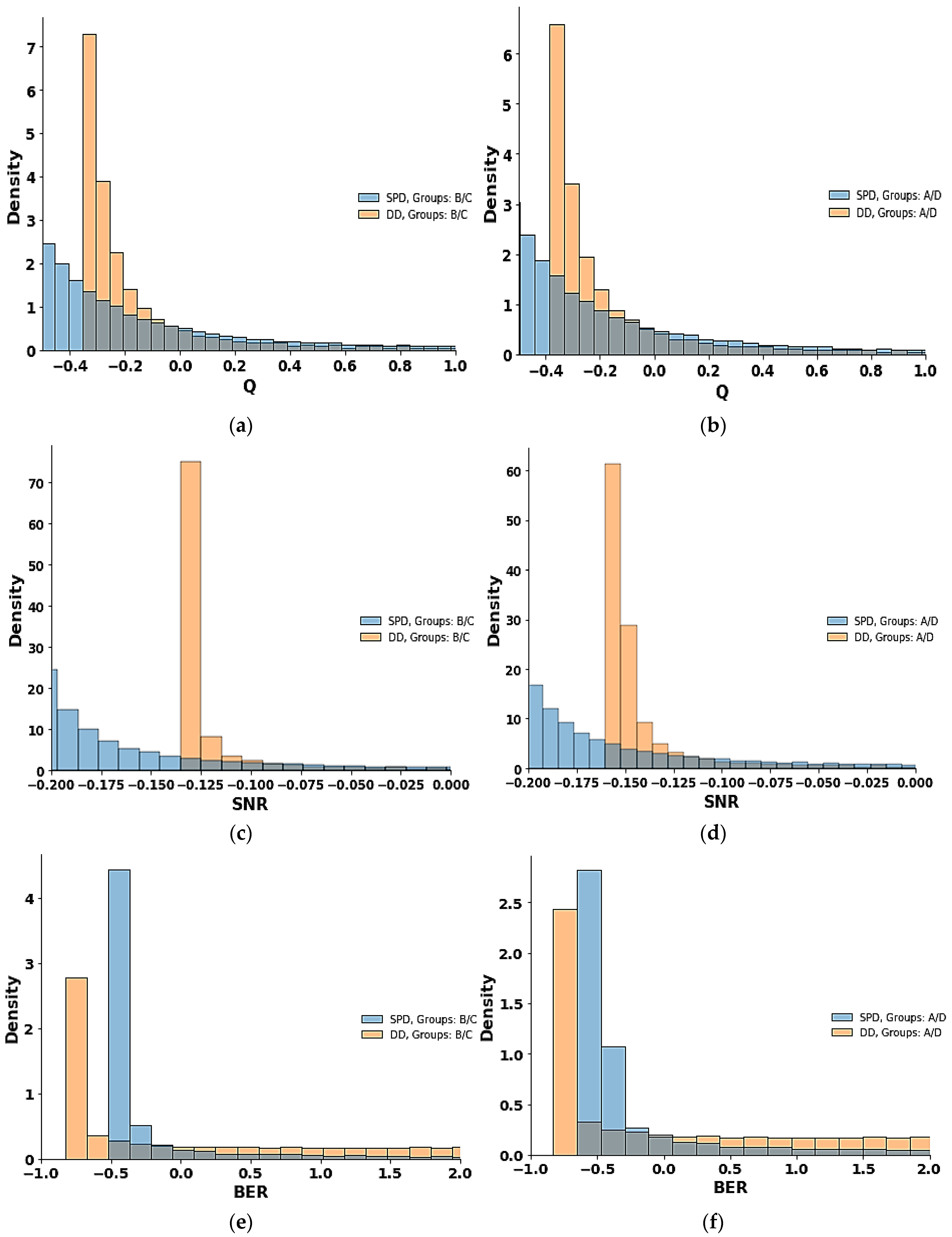
After testing the hypothesis and normalizing each feature using z-score normalization, the data are visualized through count-plot where each detection technique SPD and DD are compared within the groups A/D and B/C.
These features corresponding to each group are shown in
Figure 2.
3. ML Procedures
The ML problem formulation is to classify between different data rates at different detection techniques (DD and SPD) to achieve a certain key performance indicator (KPI) need. The KPIs’ needs are the following spectrum. We use C-band and can use it in next-generation passive optical networks (PONs), data rates (1.25 Gbps for audio and 2.5 Gbps for video). The Q, SNR and BER are used as ML predictors. The DT and RF are both used as classifiers. The classification process is formulated in order to determine four different classes with different data rates {DD: Groups A/D, DD: Groups B/C, SPD: Groups A/D, SPD: Groups B/C}. Hence, the classifiers are used as supervised learning where the training data has an output included while training the model. The total dataset rows and columns are 1800 and 4, respectively. The four columns are the Q, SNR and BER while the fourth column is the label outcome. The number of training data points is 1200 (300 data points for each class of the four classes). Then, the number of test data points is 600 (150 data points for each of the four classes).
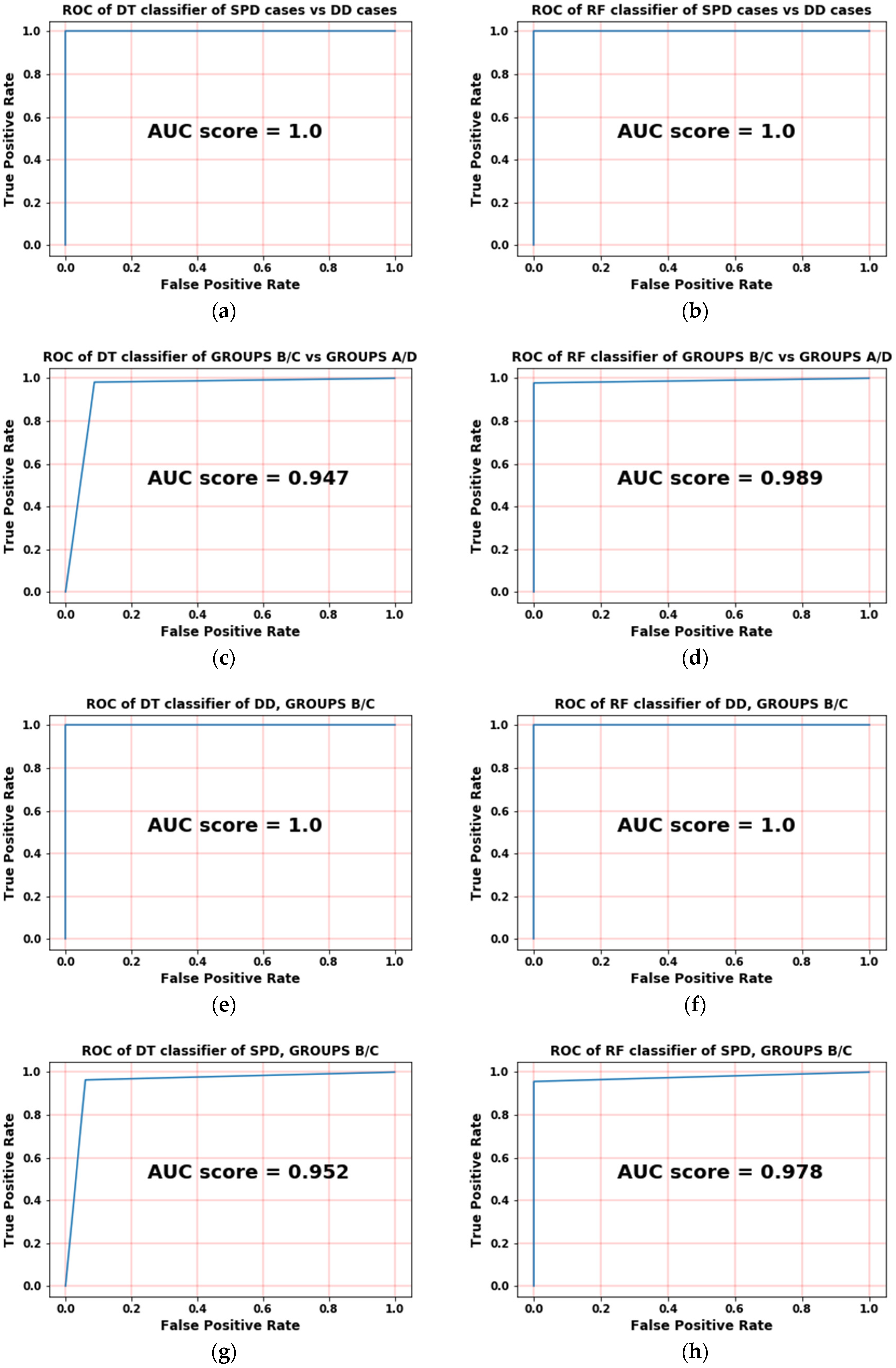
The input features of the test data Q, SNR and BER are used to test the model. Then the model-predicted labels are evaluated using the output of the test data as the true label. The evaluation is done using confusion matrices and ROC curves. First, the confusion matrix shows the relation between the actual values and predicted values. Hence, the accuracy of the model can be easily extracted from it as the accuracy is the ratio between the right predictions over the whole test set. Moreover, the ROC curves are revealed as they display the relation between the true-positive rate and the false-positive rate.
The ideal case of ROC curve occurs when the area under the curve gets to its maximum of 1. The ROC curves are binary. This means that it can be used in binary classification. As such, each unique case is shown versus the other 3 cases, e.g., DD: Groups B/C versus DD: Groups A/D, SPD: Groups B/C and SPD: Groups A/D, so that the problem formulation turns into binary classification in order to reveal each ROC curve.
3.1. Decision Tree
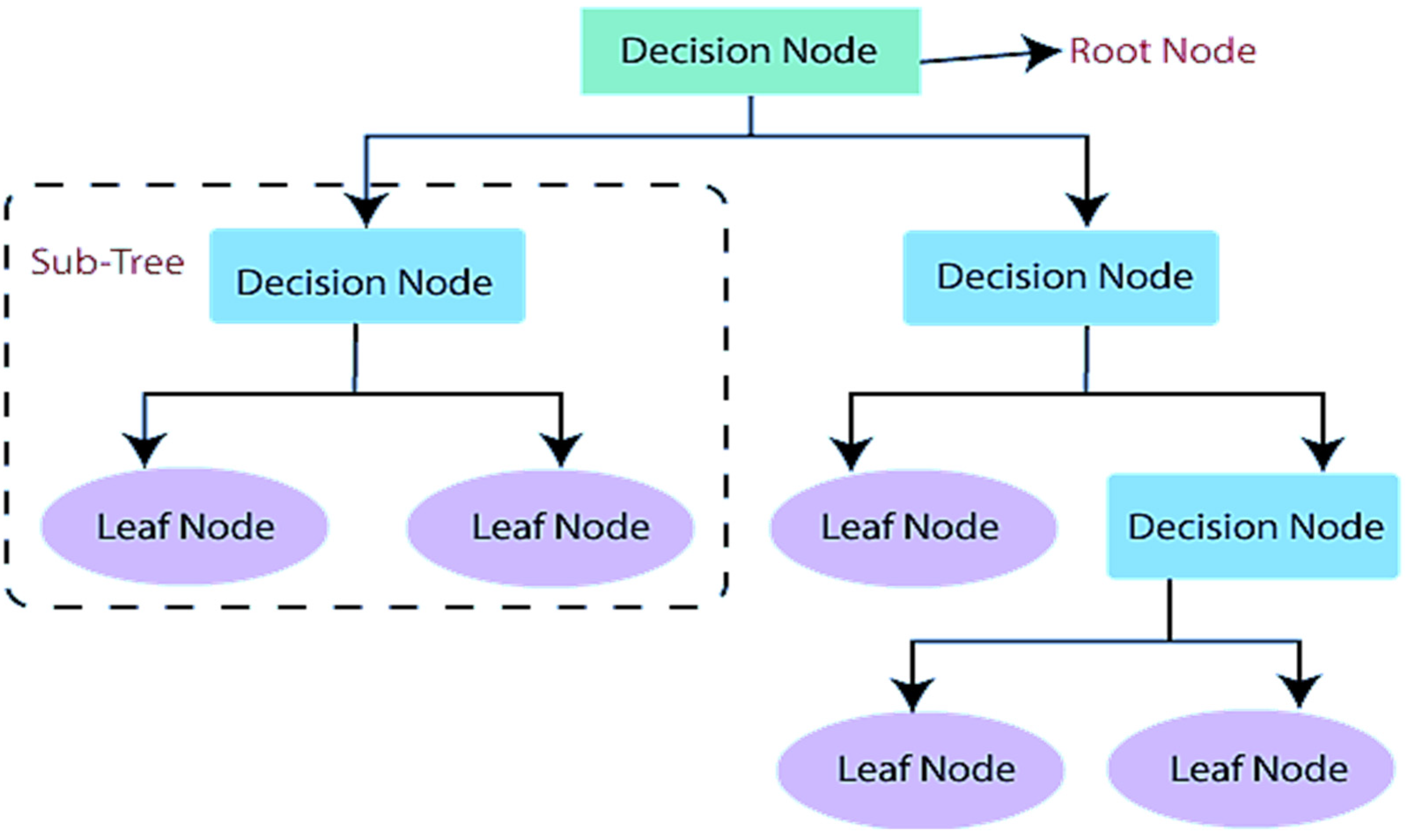
A typical type of supervised learning algorithm is the decision tree (DT). It formulates the classification model by creating a DT. Each node in the tree denotes a test on an attribute, and each branch descending from that node, represents one of the attribute potential values [
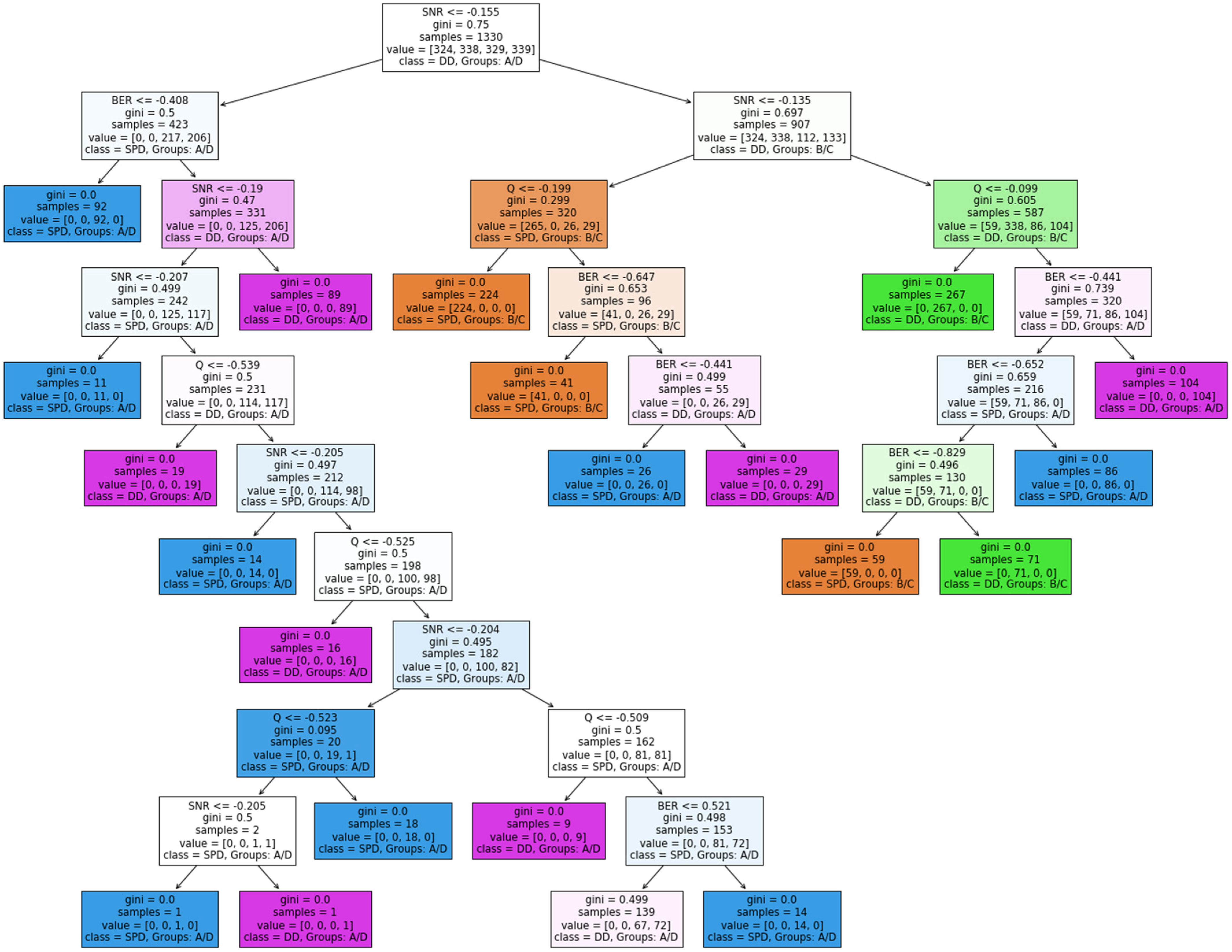
15]. In a DT, there are two nodes, which are the decision node and leaf node. Each leaf node represents the result, while the internal nodes indicate the dataset’s features and branches its decision-making processes, as shown in
Figure 3.
A major advantage of the DT is solving the nonlinear classification problems. It is capable of formulating nonlinear decision boundaries, unlike the linear decision boundaries, so the DT solves more complex problems [
16].
3.2. Random Forest
An ensemble learning technique for classification, regression, and other problems is the random forest (RF), often referred to as random choice forest, which works by creating a huge number of decision trees during training. The class that the majority of trees select is the output of the random forest for classification problems. The issue of DTs that overfit their training set is addressed by RF. So, RF typically performs better than DT [
17].
Deeply developed trees, in particular, have a tendency to acquire highly irregular patterns: they overfit their training sets, resulting in low bias but large variation [
18]. Random forests are a method of minimizing variation by averaging numerous deep decision trees trained on various regions of the same training set. This comes at the cost of a modest increase in bias and some loss of interpretability, but it significantly improves the final model’s performance.
The training algorithm for RF, adopts the technique of bagging. Assume a training set
with outcome
bagging repetitively (
N times) chooses a random sample with the replacement of the training set and fits trees [
19]:
For b = 1, …, N:
Bootstrapping samples with n training examples from X, Y; call these Xb, Yb.
Training a model tree fb on Xb, Yb.
After training, predictions for unknown samples
x′ is done by having the average predictions from all the individual trees on
x′:
4. ML Evaluation
In this section, the results of the hypothesis testing, Pearson correlation, VIF and the ML models are revealed. The confusion matrices of both classifiers are revealed. The ROC curves are displayed and discussed for all cases.
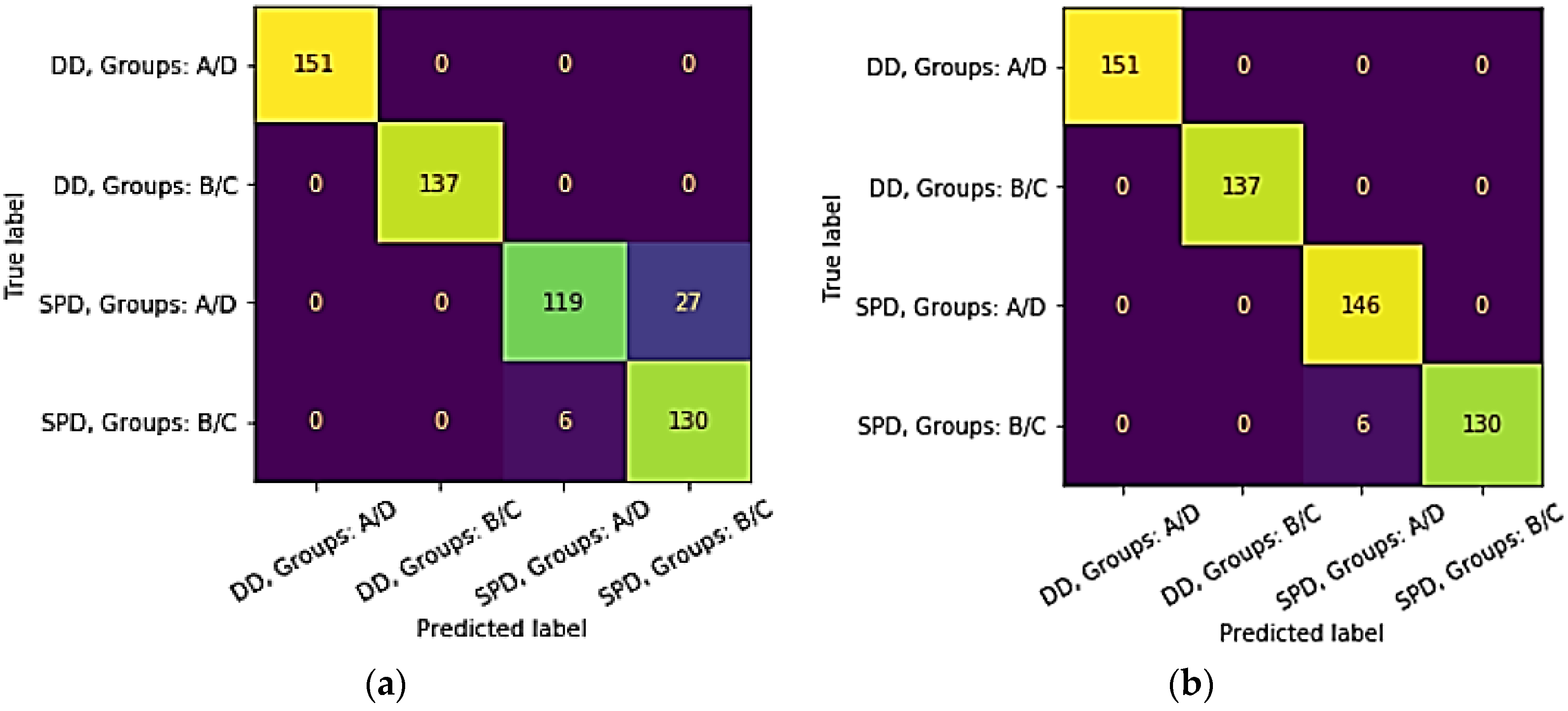
The four classes are compared in terms of the predicted outcome and the actual ones. The actual label value is represented as the true label.
Figure 4 shows the confusion matrices for both DT and RF.
As the color of each cell on the matrix diagonal gets brighter, this indicates that a perfect classification performance gets achieved.
Figure 4a shows that the DT has misclassified an overall 33 labels while the RF has only 6 misclassifications. Hence, the accuracy of the DT is 94% while the accuracy of the RF is 99%, so the preliminary results show that the RF outperforms the DT. To make sure this is correct, the ROC curves are revealed in
Figure 5. Both classifiers are compared side by side during performing the same binary classification problem.
The first case in
Figure 5a,b is the classification between SPD (both groups) and DD (both groups) where the DT and RF have shown an ideal classification as the area under the curve is nearly maximized. The second case is the classification between all Groups A/D and all Groups B/C where the RF ROC is clearly accurate than DT
Figure 5c,d.
Figure 5e,f are showing that both classifiers achieved ideal ROCs in classifying a specific output that represents the DD of Groups B/C.
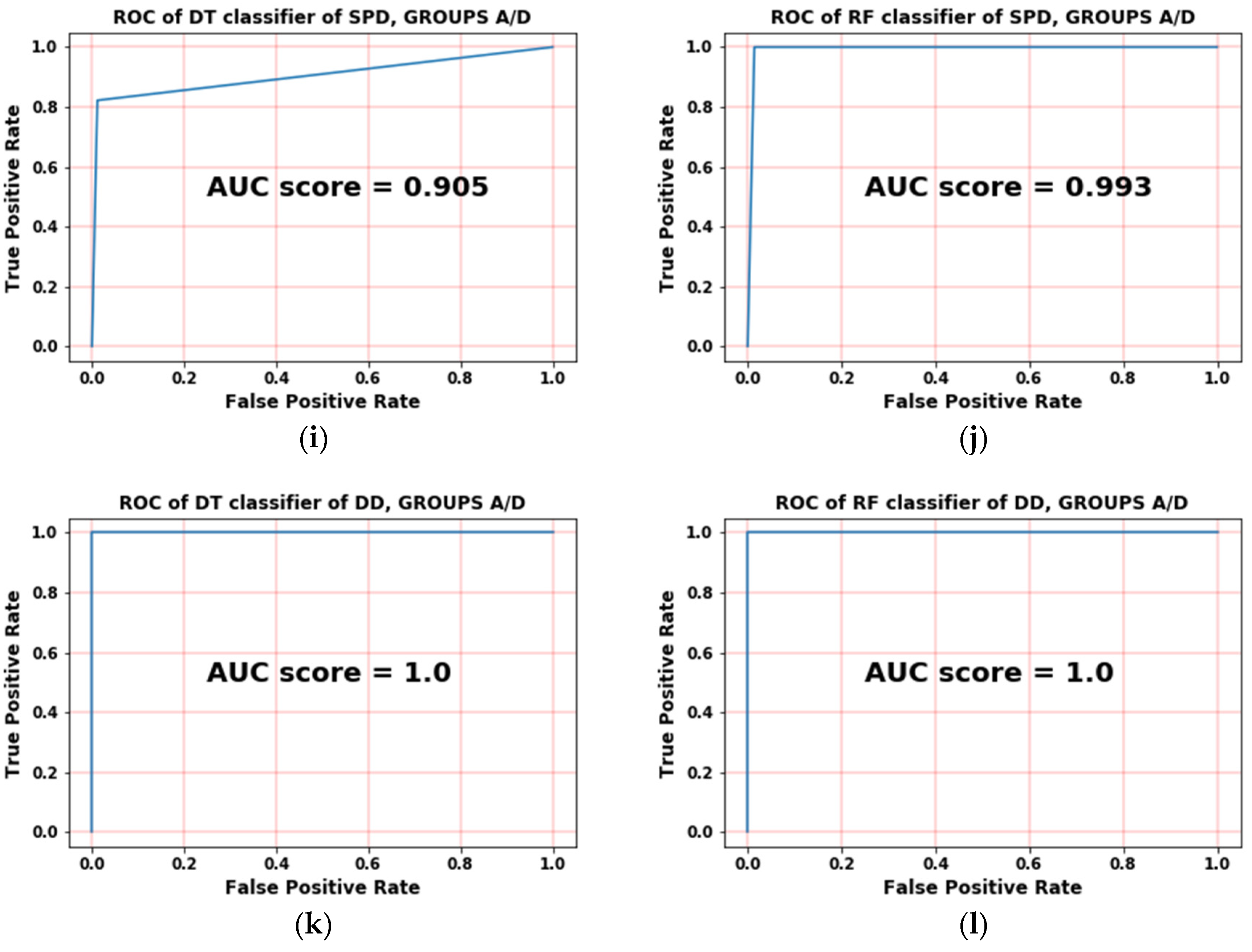
Figure 5g–j shows the classification of SPD (Groups B/C) and the classification of SPD (Groups A/D), respectively, where the RF has properly classified these cases and has shown promising near-ideal results. The final case of
Figure 5k,l shows ideal results for both classifiers RF and DT, so for each particular binary classification of ROC curves, the RF outperforms the DT.
Figure 6 shows the decision tree threshold bounding.
The leaf nodes and decision nodes are revealed after training and validating the model where the maximum depth of the tree is 10. The Gini impurity measure is a method utilized in DT algorithms to decide the optimal split from a root node. For example, in the very first few steps of the DT process, the root node has a Gini index of 0.75 for SNR less than or equal −0.155 for DD (Groups A/B). Then the root node is split into 2 decision nodes: one for BER less than or equal −0.408 and the other for SNR less than or equaling −0.135. The first decision node is split into one leaf node in which the label is decided as SPD (Groups A/D) and the others.
The procedures complete as mentioned in the very first steps where the leaf and decision nodes are completed and formed based on the threshold of the predictor and the Gini index.
5. Conclusions
The classification of different groups of QoS is done using machine learning (ML). The input predictors were studied to determine the data robustness. In terms of BER, SNR, and maximum number of users, the suggested system’s performance is analyzed analytically. Hypothesis testing is used to prove the ML input data robustness. The test showed 0.98, 0.97, and 0.98 for Q-factor, SNR, and BER, respectively. The multicollinearity of the data is studied using Pearson correlation and VIF as they are revealed for the dataset. The Q-factor has 4.8 VIF while the values for SNR and BER are 3.88 and 1.44. These results prove that each component is important for ML classification, as there is no existing multicollinearity between any components. Then, ML is used to classify whether the code weights are even or odd for both cases SPD and DD (QoS cases for video and audio). Hence, the ML is formulating a classification problem to classify four classes. ML evaluation shows promising results, as the DT and the RF classifiers achieved 94% and 99% accuracy, respectively. The ROC curves and AUC scores of each case are revealed, showing that the RF outperforms the DT classification performance. The study of other features, such as polarization and eye opening that significantly affects ML, is still under research.
Author Contributions
Conceptualization, S.A.A.E.-M. and A.M.; methodology, S.A.A.E.-M. and A.M.; software, S.A.A.E.-M. and A.M.; validation, S.A.A.E.-M., A.M., A.C., H.Y.A. and M.Z.; formal analysis, A.M., A.C., H.Y.A. and A.N.K.; investigation, S.A.A.E.-M., A.M. and H.Y.A.; resources, S.A.A.E.-M. and A.M.; writing—original draft preparation, S.A.A.E.-M. and A.M.; writing—review and editing, A.C. and H.Y.A.; visualization, A.C. and H.Y.A.; funding acquisition, A.C. All authors have read and agreed to the published version of the manuscript.
Funding
This research received no external funding.
Conflicts of Interest
The authors declare no conflict of interest.
References
- Angra, S.; Ahuja, S. Machine learning and its applications: A review. In Proceedings of the 2017 International Conference on Big Data Analytics and Computational Intelligence (ICBDAC), Cirala, India, 23–25 March 2017; pp. 57–60. [Google Scholar]
- Abdualgalil, B.; Abraham, S. Applications of machine learning algorithms and performance comparison: A review. In Proceedings of the 2020 International Conference on Emerging Trends in Information Technology and Engineering (ic-ETITE), Vellora, India, 24–25 February 2020; pp. 1–6. [Google Scholar]
- Kaur, J.; Khan, M.A.; Iftikhar, M.; Imran, M.; Emad Ul Haq, Q. Machine learning techniques for 5G and beyond. IEEE Access 2021, 9, 23472–23488. [Google Scholar] [CrossRef]
- Zaki, A.; Métwalli, A.; Aly, M.H.; Badawi, W.K. Enhanced feature selection method based on regularization and kernel trick for 5G applications and beyond. Alex. Eng. J. 2022, 61, 11589–11600. [Google Scholar] [CrossRef]
- Dat, P.T.; Kanno, A.; Yamamoto, N.; Kawanishi, T. Seamless convergence of fiber and wireless systems for 5G and beyond networks. J. Light. Technol. 2018, 37, 592–605. [Google Scholar] [CrossRef]
- Shiraz, H.G.; Karbassian, M.M. Optical CDMA Networks: Principles, Analysis and Applications; Wiley: Hoboken, NJ, USA, 2012. [Google Scholar]
- Osadola, T.B.; Idris, S.K.; Glesk, I.; Kwong, W.C. Network scaling using OCDMA over OTDM. IEEE Photon. Technol. Lett. 2012, 24, 395–397. [Google Scholar] [CrossRef]
- Huang, J.; Yang, C. Permuted M-matrices for the reduction of phase-induced intensity noise in optical CDMA Network. IEEE Trans. Commun. 2006, 54, 150–158. [Google Scholar] [CrossRef]
- Ahmed, H.Y.; Nisar, K.S.; Zeghid, M.; Aljunid, S.A. Numerical Method for Constructing Fixed Right Shift (FRS) Code for SAC-OCDMA Systems. Int. J. Adv. Comput. Sci. Appl. (IJACSA) 2017, 8, 246–252. [Google Scholar]
- Kitayama, K.-I.; Wang, X.; Wada, N. OCDMA over WDM PON—Solution path to gigabit-symmetric FTTH. J. Lightw. Technol. 2006, 24, 1654. [Google Scholar] [CrossRef]
- Vu, M.T.; Oechtering, T.J.; Skoglund, M. Hypothesis testing and identification systems. IEEE Trans. Inf. Theory 2021, 67, 3765–3780. [Google Scholar] [CrossRef]
- Raju, V.N.G.; Lakshmi, K.P.; Jain, V.M.; Kalidindi, A.; Padma, V. Study the influence of normalization/transformation process on the accuracy of supervised classification. In Proceedings of the 2020 Third International Conference on Smart Systems and Inventive Technology (ICSSIT), Tirunelveli, India, 20–22 August 2020; pp. 729–735. [Google Scholar]
- Zhi, X.; Yuexin, S.; Jin, M.; Lujie, Z.; Zijian, D. Research on the Pearson correlation coefficient evaluation method of analog signal in the process of unit peak load regulation. In Proceedings of the 2017 13th IEEE International Conference on Electronic Measurement & Instruments (ICEMI), Yangzhou, China, 20–22 October 2017; pp. 522–527. [Google Scholar]
- Shah, I.; Sajid, F.; Ali, S.; Rehman, A.; Bahaj, S.A.; Fati, S.M. On the Performance of Jackknife Based Estimators for Ridge Regression. IEEE Access 2021, 9, 68044–68053. [Google Scholar] [CrossRef]
- Navada, A.; Ansari, A.N.; Patil, S.; Sonkamble, B.A. Overview of use of decision tree algorithms in machine learning. In Proceedings of the 2011 IEEE Control and System Graduate Research Colloquium, Shah Alam, Malaysia, 27–28 June 2011; pp. 37–42. [Google Scholar]
- Al Hamad, M.; Zeki, A.M. Accuracy vs. cost in decision trees: A survey. In Proceedings of the 2018 International Conference on Innovation and Intelligence for Informatics, Computing, and Technologies (3ICT), Sakhier, Bahrain, 18–20 November 2018; pp. 1–4. [Google Scholar]
- More, A.S.; Rana, D.P. Review of random forest classification techniques to resolve data imbalance. In Proceedings of the 2017 1st International Conference on Intelligent Systems and Information Management (ICISIM), Aurangabad, India, 5–6 October 2017; pp. 72–78. [Google Scholar]
- Xiao, Y.; Huang, W.; Wang, J. A random forest classification algorithm based on dichotomy rule fusion. In Proceedings of the 2020 IEEE 10th International Conference on Electronics Information and Emergency Communication (ICEIEC), Beijing, China, 17–19 July 2020; pp. 182–185. [Google Scholar]
- Paul, A.; Mukherjee, D.P.; Das, P.; Gangopadhyay, A.; Chintha, A.R.; Kundu, S. Improved random forest for classification. IEEE Trans. Image Process. 2018, 27, 4012–4024. [Google Scholar] [CrossRef] [PubMed]
| Publisher’s Note: MDPI stays neutral with regard to jurisdictional claims in published maps and institutional affiliations. |
© 2022 by the authors. Licensee MDPI, Basel, Switzerland. This article is an open access article distributed under the terms and conditions of the Creative Commons Attribution (CC BY) license (https://creativecommons.org/licenses/by/4.0/).


 ,
, 


