Enhancement of Underwater Images by CNN-Based Color Balance and Dehazing

Abstract

Convolutional neural networks (CNNs) are employed to achieve the color balance and dehazing of degraded underwater images. In the module of color balance, an underwater generative adversarial network (UGAN) is constructed. The mapping relationship between underwater images with color deviation and clean underwater images is learned. In the module of clarity improvement, an all-in-one dehazing model is proposed in which a comprehensive index is introduced and estimated by deep CNN. The third module to enhance underwater images adopts an adaptive contrast improvement method by fusing global and local histogram information. Combined with several underwater image datasets, the proposed enhancement method based on the three modules is evaluated, both by subjective visual effects and quantitative evaluation metrics. To demonstrate the advantages of the proposed method, several commonly used underwater image enhancement algorithms are compared. The comparison results indicate that the proposed method gains better enhancement effects for underwater images in different scenes than the other enhancement algorithms, since it can significantly diminish the color deviation, blur, and low contrast in degraded underwater images.

1. Introduction

Underwater information plays an important role in the human exploration and exploitation of the underwater world, for example, underwater archeology [1], underwater localization [2], underwater maintenance [3], underwater target recognition [4], underwater search and salvage [5], underwater environment monitoring [6], etc. Acoustic technology and optical technology are both used to obtain underwater information. Comparatively, optical images and videos present us a more intuitive understanding of underwater objectives. However, the particularity of the underwater environment degrades the visibility and quality of underwater images, and videos, for example, suffer from resultant color deviation, blur, and decrease in contrast. The attenuation and scattering of light propagation in water partly account for the degradation. Other reasons for the degradation are because of the movement of water or underwater creatures [7], temperature and salinity [8], noises such as salt and pepper noise, Gaussian noise, and marine snow [9]. To alleviate the degradation of underwater images and videos, one can resort to advanced equipment, for example, a divergent beam underwater Lidar imaging system [10] and a multistate underwater laser line scan system [11]. However, the expense of the equipment hinders its wide use. By contrast, image processing provides an effective way to obtain high-quality images and videos at low cost. During the last decade, the enhancement and restoration of underwater images received more and more attention.

This paper aims to comprehensively enhance underwater images from the aspects of color, clarity, and contrast. To achieve this, color deviation and blur are diminished by an underwater generative adversarial network and a CNN-based all-in-one dehazing model, respectively. To further improve the contrast of underwater images, an adaptive contrast improvement method is proposed. Several commonly used underwater image enhancement algorithms are compared with the proposed algorithm, not only from the point of view of subjective visual effect but also from several quantitative evaluation metrics.

The rest of the paper is organized as follows. In Section 2, underwater image enhancement methods and the issues are reviewed. In Section 3, the fundamentals of underwater imaging and CNN are described. In Section 4, the methods proposed in the study are explained, including UGAN-based color balance, CNN-based dehazing, and adaptive contrast enhancement. In Section 5, underwater images are treated using the proposed method and the results are evaluated from quantitative and subjective aspects, and compared to other algorithms. The final section is the conclusion.

2. Literature Review

Generally, physical model-based and physical model-free approaches are available for the enhancement and restoration of underwater images. A physical model for underwater imaging gives the relationship between degraded underwater images and restored underwater images. By determining the transmittance of light and estimating the background light of the surrounding underwater environment, the restored underwater images can be obtained. A representative physical model for underwater imaging is the Jaffe–McGlamery model [12]. Based on the Jaffe–McGlamery model, Trucco and Olmos-Antillon [13] proposed a self-tuning filter for underwater image restoration. Wang et al. [14] presented an effective two-stage method to restore underwater images. Wagner et al. [15] addressed a visual quality-driven restoration method for underwater images. Shi et al. [16] proposed a normalized gamma transformation to obtain contrast restoration. Inspired by the Jaffe–McGlamery model, He et al. [17] initiated the dark channel prior (DCP) model, and this model is commonly used in underwater image restoration. Galdran et al. [18] proposed a red channel method to restore underwater images. Li et al. [19] combined gray-world and DCP to improve the color and contrast of underwater images. Tang et al. [20] presented an improved DCP algorithm to preprocess underwater monocular vision images. Xie et al. [21] used background light estimation and DCP to obtain underwater image restoration. Yu et al. [22] proposed a DCP-based underwater image dehazing algorithm by combining homomorphic filtering, double transmission map, and dual-image wavelet fusion.

Compared with physical model-based enhancement and restoration of underwater images, the physical model-free approach provides a more direct way to enhance the underwater images since its focus is on the adjustment of pixels of underwater images. Representative techniques involve white balance [23], gamma correction [7], histogram equalization [24], wavelet transformation [25], and the Retinex algorithm [26]. Due to the diversity of the degradation of underwater images (as aforementioned color deviation, blur, and decrease in contrast), researchers prefer to combine two or more techniques to obtain comprehensive high-quality underwater images. Examples are the integration of histogram equalization and wavelet transformation [27,28], the fusion of white balance, histogram equalization, and wavelet transformation [29], as well as the combination of histogram equalization, white balance, and gamma correction [30]. Moreover, it is noted that in much research, the physical model is also considered when a physical model-free method is used, which means the combination of the physical model-based approach and physical model-free approach. For example, Li et al. [31] proposed the enhancement of underwater images by dehazing with minimum information loss and histogram distribution prior. Wending et al. [32] presented the underwater image enhancement based on red channel weighted compensation and gamma correction. Wang et al. [33] addressed a L2-based Laplacian pyramid fusion algorithm. Luo et al. [34] proposed a fusion algorithm with color balance, contrast optimization, and histogram stretching.

During the last decade, the development of artificial intelligence (AI) provided new tools for image processing. Representative examples are neural networks (NN) and support vector machines (SVM). Both NN and SVM show their ability in image enhancement. With the rapid progress in computer science and technology, in recent years a machine learning method, deep learning, was paid considerable attention, since it presented powerful learning or calculation ability in many areas, for example, underwater image enhancement. Singh et al. [35] and Arif et al. [36] review the application of deep learning to image enhancement, especially the image dehazing. Manzo and Pellino [37] adopted a pretrained deep neural networks-based architecture for image description, and subsequently, classification. Li et al. [38] applied a deep neural network to the underwater image de-scattering. Perez et al. [39] proposed a deep convolutional neural network (CNN) to dehaze underwater images. Wang et al. [40] used deep CNN for the color correction and haze removal of underwater images. Saeed et al. [41] presented the reconstruction of clear latent underwater images by using deep CNN. Wang et al. [42] proposed a parallel deep CNN to estimate the transmission and light in restoring underwater images. Mhala and Pais [43] presented a secure visual secret sharing scheme combined with CNN to enhance underwater images. Due to the difficulty with the ground truth of underwater images, normal deep learning structure is limited to dealing with specific underwater images associated with ground truth. To solve the problem, a generative adversarial network (GAN), in which CNN is commonly adopted, was recently applied to the enhancement of underwater images. By using GAN, training samples can be enriched significantly so that deep learning performs well. Fabbri et al. [44] presented the improvement of visual underwater scenes by using GAN. Li et al. [45] reported real-time color correction of underwater images by an unsupervised GAN (Water-GAN). Liu et al. [46] used a cycle-consistent generative adversarial network (CycleGAN) to generate underwater images as training data for CNN models for enhancement. Guo et al. [47] addressed a multiscale dense GAN for enhancing underwater images. Yang et al. [48] proposed a multi-scale generator-based conditional GAN to obtain clear underwater images. Zhang et al. [49] proposed an improved GAN to deal with the color restoration of underwater images. Liu et al. [50] addressed the integration of GAN and the Akkaynak–Treibitz model in the enhancement of underwater images.

In general, CNN-based underwater image enhancement and restoration achieved some progresses in recent years. Nevertheless, the power of CNN is to be further exploited. In the study, CNN is employed to enhance underwater images from two aspects, i.e., the color balance and dehazing. Although it was proven that GAN is predominant in diminishing the color deviation of underwater images (e.g., [45,49]), two points should be addressed further when using GAN. One is with the dataset used in GAN. Usually the set of ground truth is small-scale, which limits the enhancement effect by GAN. The other point is that other properties of underwater images actually need to be further improved, such as clarity and contrast, since the specialty of GAN is to deal with color deviation. In the study, an augmented ground truth is constructed by combining two underwater datasets, i.e., Imagenet [51] and EUVP [52]. To improve the clarity of underwater images, an all-in-one dehazing model is proposed to reduce the accumulated errors that result from determining the transmittance and background light individually when a conventional restoration model is used. In the all-in-one dehazing model, a comprehensive index that involves transmittance and background light is identified by a deep CNN. After the treatment of color deviation by GAN and dehazing by CNN, the underwater images are further enhanced by improving contrast. An adaptive contrast enhancement algorithm is proposed by fusing global and local contrast information. In summary, in the study a hybrid enhancement method is proposed in which both a physical model-based approach and a physical model-free approach are used. In detail, GAN-based color balance and contrast enhancement can be viewed as physical model-free approaches, while CNN-based dehazing can be viewed as a physical model-based approach. The highlights mainly refer to the augmentation of ground truth, color balance by GAN, use of CNN in the all-in-one dehazing model, and the fusion algorithm in the contrast improvement. To verify the proposed image enhancement method, a lot of underwater images from datasets are dealt with, and some of the results are presented. The novelty of the study mainly refers to the combination of deep learning-based underwater image enhancement and conventional enhancement. Existing deep learning-based enhancement methods for underwater images usually focus on the color balance or dehazing, while the contrast improvement is ignored. The main contributions of the paper include (1) an augmented dataset-based GAN proposed for the color balance of underwater images; (2) a CNN-based all-in-one model proposed to the dehazing of underwater images; (3) and an adaptive contrast improvement that combines adjustable histogram equalization and contrast limited adaptive histogram equalization is for the contrast enhancement of underwater images.

3. Fundamentals

3.1. Underwater Imaging

The propagation of light in water is affected by underwater environments, which results in the attenuation and scattering of light. Influence factors refer to the density of water, selective refraction and absorption of light by water, underwater suspended particles, movement of water, the temperature, and the salinity of water. Consequently, optical underwater images commonly have the problems of color deviation, blur, and low contrast.

Due to the attenuation and scattering of light in underwater imaging, the received light intensity by a camera can be described as the sum of three parts:

$$I=E_d+E_f+E_b,$$

(1)

where I denotes the total light intensity; E_d denotes the part of direct reflection of light; E_f denotes the part of forward scattering of light; E_b denotes the part of backward scattering of light. For the direct part E_d, no scattering of light is considered but the attenuation. The model of E_d is

$$E_d(x)=J(x)e^{-cd(x)}=J(x)t(x),$$

(2)

where J(x) denotes the light received from an illumination source to the object; c is the coefficient of the attenuation of light; d(x) is the distance between the sensor (e.g., camera) and the underwater object. t(x) is introduced as the transmittance with definition $t\left(x\right)=e^{-cd\left(x\right)}.$

For the forward scattering of light E_f, it relates to the disturbed reflection of light from an object. A representative disturbance is the underwater suspended particles. For small-angle scattering, E_f can be calculated as a convolution [53],

$$E_f(x)=E_d(x)\ast g(x)=(J(x)t(x))\ast g(x),$$

(3)

where g(x) is the point spread function (PSF).

For the backward scattering of light E_b, it derives from the reflection by underwater suspended particles instead of the object to be imaged. Therefore, it can be viewed as a noise in the underwater imaging model (1). The model of E_b is

$$E_b(x)=B_{\infty }(x)(1-t(x)),$$

(4)

where B_∞ is the water background.

According to the Equations (2)–(4), the received light intensity by a camera expressed as (1) can be rewritten as

$$I(x)=J(x)t(x)+(J(x)t(x))\ast g(x)+B_{\infty }(x)(1-t(x)),$$

(5)

Usually, the contribution of the forward scattering of light E_f in the model (1) is much less than that of the direct reflection E_d, and the backward scattering of light E_b, especially when the image plant is close to the object to be imaged. Therefore, the model (5) can be simplified as

$$I(x)=J(x)t(x)+B_{\infty }(x)(1-t(x)),$$

(6)

Equation (6) is often used as a restoration model in image processing. J(x) represents a restored image, while I(x) represents the real image received by a sensor-like camera. As aforementioned, t(x) relates to the attenuation of light in water while the second term in (6), i.e., $B_{\infty }\left(x\right)\left(1-t\left(x\right)\right)$ represents the backward scattering of light in water. In an idealistic case, when the attenuation and scattering of light in water disappears, obviously I(x) = J(x) holds. However, in real underwater imaging environments, the attenuation and scattering of light are inevitable and have to be considered. As can be inferred from (6), the restored image J(x) depends on t(x) and $B_{\infty }\left(x\right)$ after I(x) is obtained by a sensor. Some methods were proposed to obtain t(x) and $B_{\infty }\left(x\right)$, for example, the maximum intensity prior [54,55]; DCP [56,57]; red channel prior [18]; image blurring and light absorption [58]; and underwater light attenuation prior [59].

3.2. Convolutional Neural Network (CNN)

As a kind of artificial neural network, convolution neural network (CNN) is most commonly employed to analyze visual images. Examples of classical CNNs are LeNet-5, AlexNet, Inception, ResNet, and VGGNet. Based on the shared weight architecture of filters, CNN is of low complexity and little pre-processing. Moreover, due to the equivariant and invariant characteristics, CNN guarantees the stability in processing images. A typical CNN architecture consists of an input layer, convolutional layers, pooling layers, a full connection layer, and an output layer, as shown in Figure 1. In the example figure, 3 × 3 and 2 × 2 represent the size of convolutional kernel. When CNN is used in image processing, images are taken as inputs. Convolution is performed to extract features in images by filters and the features are further mapped by pooling. In the full connection layer, all features are collected to form the final output images.

As a vital component, the filter in CNN can be viewed as shared weights to extract the features in images. For different features, different filters can be selected. Given an input image $X=\left\{x_{pq}\right\}\in R^{M\times N}$ and the filter $W=\left\{w_{uv}\right\}\in R^{u\times v}$, suppose the stride = 1, standard convolution operation yields $Y=\left\{y_{ij}\right\}$ as

$$y_{ij}={\displaystyle \sum _{u=1}^U{\displaystyle \sum _{v=1}^V{w}_{uv}{x}_{i-u+1,j-v+1}}},$$

(7)

Activation functions, such as ReLU (rectified linear unit), are then employed to increase the nonlinear property of CNN. Thus, feature maps can be obtained. Afterwards, another important component, pooling, is conducted. Commonly used pooling concerns average pooling and max pooling, by which the size of the feature map can be reduced. Moreover, the problem of over-fit can be avoided by pooling. After several convolutional layers and pooling layers, the full connection layer performs a high-level reasoning to form the final output image. In this layer, all local features obtained in the convolutional layers are collected and the neurons between different layers are fully connected, as seen in regular ANN.

4. Underwater Image Enhancement by UGAN-Based Color Balance, CNN-Based Dehazing and Adaptive Contrast Enhancement

A sketch that depicts the procedure of the proposed underwater image enhancement is shown as Figure 2. As can be seen, CNN is employed in the color balance and dehazing while contrast improvement is conducted afterwards. The enhancement is conducted by three steps, i.e., color balance, dehazing, and contrast improvement. Firstly, CNN is used to form a higher-level architecture, i.e., UGAN to correct the color deviation of degraded underwater images. Secondly, to solve the problem of blur and the low definition of underwater images, a CNN-based integrated dehazing model is proposed. Finally, an adaptive contrast enhancement algorithm based on the fusion of global and local contrast information is used to improve the contrast of the underwater image.

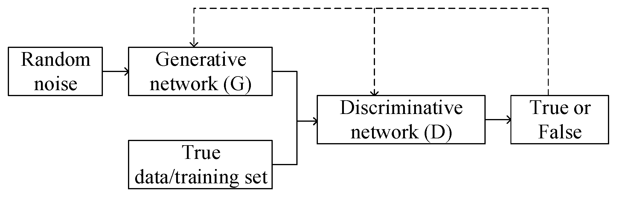
4.1. Color Balance by Underwater Generative Adversarial Network (UGAN)

A representative application of CNN is to construct generative adversarial networks. A generative adversarial network (GAN) is a framework for obtaining generative models in the form of a contest conducted by a generative network and discriminative network [60]. The framework operates in the manner of unsupervised learning. In the GAN structure, the mission of the discriminative network is to identify the realness of data, while the mission of generative network is to successfully cheat the discriminative network by creating realistic-looking data. Such a zero-sum game lasts until the generative network wins. The structure of GAN can be depicted as Figure 3. A well-trained discriminative network (D) is connected with a generative network (G) that will be updated until the discriminative network cannot distinguish whether the data are from a true training set or the sample generated by a generative network. Such a contest can be modeled as a minimax optimization, i.e.,

$$\underset{G}{\min }\underset{D}{\max }\left\{\underset{{}_{x~P_{data}(x)}}{\mathbb{E}}[\log (D(x))]+\underset{{}_{z~P_z(z)}}{\mathbb{E}}[\log (1-D(G(Z)))]\right\},$$

(8)

where $P_{data}$ represents the distribution over true data, while  is the prior on random noise. D(x) denotes the probability if x derives from true data. G(z) is the synthetic image.

During past years, GAN found increasing applications in the areas of art, science, and even games. The majority of GAN applications are with image processing and CNN is preferred in forming the generator and discriminator. In the study, GAN is employed to enhance underwater images. With this goal, the inputs to the generative network can be selected as low-quality or degraded underwater images while the outputs of generative network would be enhanced underwater images provided a well-trained GAN is obtained. Due to the same dimension of output images as the input images, the U-net architecture is selected in constructing the generative network. The U-net is a kind of fully convolutional network. It can be viewed as a combination of encoder and decoder, as shown in Figure 4a. In the encoder module, downsampling is performed along the contracting path. The spatial information is reduced, while feature information is increased. In the decoder module, the feature and spatial information are combined through upsampling and skip connection (concatenation) with high-resolution features from the contracting path in the encoder. In the study, the size of the input images is selected as 256 × 256. Each contraction step consists of 4 × 4 filtering with stride 2 followed by Leaky-ReLU activation and batch normalization (BN). In the decoder, the activation function is selected as ReLU.

In the discriminative network, PatchGAN is selected as the network architecture. As a Markovian discriminator, PatchGAN was proven to be a better discriminator than regular GAN for the purpose of image processing, especially in terms of image resolution and image details. The main difference is that regular GAN discriminator outputs a scalar that represents the input image is real or fake, while for PatchGAN, its discriminator outputs a matrix in which each element represents a patch (receptive field) in the input image that is real or fake. In the study, the size of the output of the discriminator is 32 × 32. Each convolution layer consists of 4 × 4 filtering with stride 2 along with Leaky-ReLU activation. The architecture of discriminator in the GAN is depicted as Figure 4b. The width and height of the boxes represent the width and height of the feature map, and different boxes correspond to different convolutional layers of the network.

The loss functions used to train the discriminator and generator are selected as Wasserstein GAN (WGAN) function and L1-norm, respectively. To improve the stability of training, a penalty term is added to the WGAN. Based on (8), the overall loss function in the UGAN can be described as

$$L_{UGAN}=L_{WGAN}(G,D)+{\lambda }_1{L}_{L1}(G),$$

(9)

where λ₁ is a weight factor and the loss function with penalty term is defined as

$$L_{WGAN}(G,D)=\mathbb{E}[D(x)]-\mathbb{E}[D(G(Z))]+{\lambda }_{\mathrm{GP}}{\mathbb{E}}_{\widehat{x}~P_{\widehat{x}}}[{({\Vert {\nabla }_{\widehat{x}}D(\widehat{x})\Vert }_2-1)}^2],$$

(10)

where λ_GP is the penalty coefficient and $P_{\widehat{x}}$ is obtained by sampling uniformly along straight lines between $P_{data}$ and $P_z$. The loss function for generator in the Equation (9) is defined as

$$L_{L1}(G)=\mathbb{E}\left[{\Vert x-G(Z)\Vert }_1\right].$$

(11)

It is noted that in the applications of GAN, some focused on the generation of realistic underwater images by GAN (e.g., [45]), while some employed GAN to the color correction of underwater images (e.g., [49]). In this paper, GAN is used for the color balance of underwater images. Similar to [49], the generator network in the study is a full convolutional encoder–decoder and U-net architecture is used. Different from [49], in the study, PatchGAN structure is used as the discriminator to guarantee the image resolution and image details.

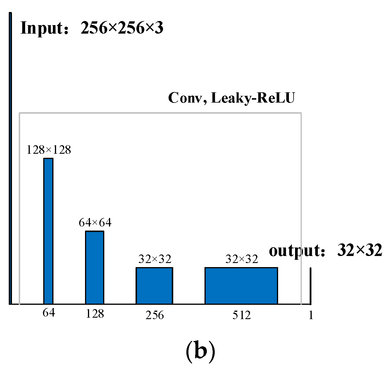
4.2. CNN-Based Integrated Dehazing Model

The model (6) originated from the treatment of images from an air environment. Now it is widely used in underwater image processing to obtain a clean or restored image J(x). Based on (6), the clean image can be determined by

$$J(x)=\frac{I(x)}{t(x)}-\frac{B_{\infty }(x)}{t(x)}+B_{\infty }(x).$$

(12)

As can be inferred, to obtain a clean image J(x), t(x), and $B_{\infty }\left(x\right)$ should be estimated in advance. Accumulated errors result from estimating t(x) and $B_{\infty }\left(x\right)$ individually. In the study, a comprehensive index is used to decrease such errors. Based on (12), an all-in-one dehazing model can be defined as

$$J(x)=K(x)I(x)-K(x)+b,$$

(13)

where b is a constant and K(x) is determined by t(x) and $B_{\infty }\left(x\right)$ as

$$K(x)=\frac{(I(x)-B_{\infty }(x))/t(x)+(B_{\infty }(x)-b)}{I(x)-1}.$$

(14)

It is obvious from the definition (13) that the clean image J(x) depends on the estimation of K(x), which is achieved by using deep CNN in the study, as shown in Figure 5.

In constructing the CNN for estimating K(x), multi-scale networks are designed to increase the accuracy and efficiency of estimation. Moreover, a coarse-scale network is concatenated with a fine-scale network to decrease the information loss during convolution operation. In the study, five convolutional layers are designed and concatenation is performed among the convolutional layers. As can be recognized from Figure 6, there is a concatenation between the first and second convolutional layers (as labelled by the black line); and between the second and third convolutional layers as well (as labelled by red line). The last concatenations are based on the first four layers (as labelled by the blue line).

The size of the filter in the first convolutional layer (denoted by con1 in Figure 6) is selected as 1 × 1, 3 × 3 in the second layer (con2), 5 × 5 in the third layer (con3), 7 × 7 in the fourth layer (con4); and 3 × 3 in the last layer (con5). The activation function is selected as RELU. Furthermore, to guarantee that the size of the output is the same as the input image, in the study the padding varies with the size of the filter in different convolutional layers, which simplifies the network structure, compared with the required pooling and upsampling operation in the case of constant padding.

According to the relationship in the convolution operation that is

$$W=\frac{N-F+2P}{S}+1,$$

(15)

the padding can be determined as

$$P=\frac{NS-N+F-S}{2},$$

(16)

in the case of N = W, where N represents the size of the input image; W the size of the output image; F the size of the filter; S the stride; and P the padding. Usually, the value of stride can be kept as 1. Therefore, the calculation of the padding can be simplified as

$$P=\frac{F-1}{2}.$$

(17)

In this way, the paddings in the five convolutional layers are 0, 1, 2, 3, and 1, respectively.

4.3. Adaptive Contrast Improvement of Underwater Images

Due to the particularity of underwater environments, the contrast of underwater images are usually low. Conventional means, such as histogram equalization (HE) do not perform well and some unexpected effects will happen, such as excessive enhancement, artifacts, and distortion. To further improve the details of underwater images, in the study an adaptive contrast improvement is proposed. Figure 7 presents the procedure. The core of the approach to contrast improvement is the histogram treatment that is composed of adjustable histogram equalization (AHE) and contrast limited adaptive histogram equalization (CLAHE). Preprocess includes linear stretching and transformation, while postprocess mainly refers to a fusion algorithm under a hue-preserving framework. The fusion algorithm combines the image obtained by AHE and the image obtained by CLAHE.

Liner stretching is to make the pixel value be within the range of [0, 255] by using the expression

$${\widehat{X}}_c=255\times \frac{X_c-X_{\min }}{X_{\max }-X_{\min }}.$$

(18)

where $c\in \left\{r,g,b\right\}$; X_max and X_min are the maximal pixel value and minimal pixel value, respectively. Furthermore, transformation from RGB image to grayscale image is performed by using the expression [61].

$$I=0.222\cdot {\widehat{X}}_R+0.707\cdot {\widehat{X}}_G+0.071\cdot {\widehat{X}}_B.$$

(19)

Normalization is then conducted to histogram h by

$$h_{\mathrm{I}}(s)=\frac{n_s}{N},$$

(20)

where n_s is the number of the pixels that have the same scale value s; N is the number of all pixels. A uniformly distributed histogram h_U can be obtained on the basis of h_I. The size of h_U is the same as h_I and each element in h_U is 1/256. Different from the standard HE, adjustable histogram equalization (AHE) is used in the study by optimizing

$$\tilde{h}=\underset{h}{\arg \min }({\Vert h-h_{\mathrm{I}}\Vert }_2^2+\lambda {\Vert h-h_{\mathrm{U}}\Vert }_2^2).$$

(21)

where λ is a trade-off parameter. The solution of the above quadratic optimization problem is

$$\tilde{h}=(\frac{1}{1+\lambda })\times h_{\mathrm{I}}+(\frac{\lambda }{1+\lambda })\times h_{\mathrm{U}}.$$

(22)

To obtain a proper λ, a tone distortion index is used [62]

$$D(T)=\underset{0\le j\le i\le 255}{\max }\left\{i-j;T(i)=T(j),h_I(i)>0,h_I(j)>0\right\},$$

(23)

where T is the transfer function in contrast enhancement. A smaller tone distortion D indicates a smoother tone of the images reproduced by T. Therefore, the trade-off parameter λ can be determined by

$$\lambda =\min D(T).$$

(24)

By using the above AHE, the contrast of an image can be improved globally. However, this global approach to contrast enhancement might not be suitable for the case when local details of an image are necessary. Therefore, in the study a local contrast enhancement technique, the contrast limited adaptive histogram equalization (CLAHE), is combined with the AHE to comprehensively improve the contrast of underwater images. Moreover, to avoid the gamut problem caused by linear stretching (Equation (18)) and transformation from RGB space to grayscale space (Equation (19)), a hue-preserving framework is adopted in the contrast enhancement. The algorithm of the hue-preserving can be expressed as

$$G_c(k)=\{\begin{array}{l}\frac{G_I(k)}{I(k)}\stackrel{\wedge }{X_c}(k),\hspace{1em}\hspace{1em}\hspace{1em}\hspace{1em}\hspace{1em}\hspace{1em}\hspace{1em}\hspace{1em}\hspace{1em}\mathrm{if}\frac{G_I(k)}{I(k)}\le 1\\ \frac{255-G_I(k)}{255-I(k)}(\stackrel{\wedge }{X_c}(k)-I(k))+G_I(k),\hspace{1em}\mathrm{if}\frac{G_I(k)}{I(k)}>1\end{array}$$

(25)

where G_I(k) is the image processed by global or local contrast enhancement.

After the global contrast enhancement by AHE, the local contrast enhancement by CLAHE, and treatment by hue preservation (HP) by Equation (25), the channels of the image can be obtained by fusion of

$$Y_{\mathrm{c}}(k)={\widehat{W}}_A(k)\times A_c(k)+{\widehat{W}}_P(k)\times P_c(k),c\in \left\{R,G,B\right\},$$

(26)

where A_c is the image processed by AHE and HP while P_c is the image processed by CLAHE and HP. The weights ${\widehat{W}}_A(k)$ and ${\widehat{W}}_P(k)$ are determined by

$${\widehat{W}}_d=\frac{W_d}{W_A+W_P},d\in \left\{A,P\right\},$$

(27)

where W_d is determined by the contrast measure C_d and the well-exposedness measure B_d

$$W_d=\min \left\{C_d,B_d\right\},d\in \left\{A,P\right\}.$$

(28)

5. Results and Analysis

To evaluate the proposed image enhancement measures, several underwater datasets are used and the evaluation is performed from both subjective and quantitative aspects. Datasets include Imagenet [51], EUVP [52], NYU2 [63], and RUIE [64]. The Imagent dataset is a large visual database designed for visual object recognition, in which more than 14 million images are contained. The EUVP dataset is constructed for enhancement of underwater visual perception, which contains a paired and an unpaired collection of 20 K underwater images of poor and good perceptual quality. The NYU2 dataset consists of more than 400 K images, containing 35,064 distinct objects, covering 894 different classes. The RUIE dataset, containing over 4000 images, is constructed as a large-scale underwater benchmark under natural light, and targets tasks including visibility degradation, color cast, and higher-level detection/classification. From the datasets Imagenet and EUVP, UGAN for color balance is trained and validated. A total of 13,863 images are used as a training set, while 2513 images are used for validation. From the dataset NYU2, CNN for dehazing is trained and validated. The training set includes 24,443 images, while 2813 images are for validation. Based on the UGAN, CNN, and the contrast enhancement proposed, images from the dataset RUIE are evaluated and compared with six conventional and commonly used algorithms in underwater image processing, including multi-scale retina enhancement algorithm with color restoration (MSRCR) [65], red channel prior (RCP) [18], underwater dark channel prior (UDCP) [15], ICM integrated color model (ICM) [24], relative global histogram stretching (RGHS) [66], and Retinex and multilayer perceptron (R-MLP) [67]. The comparison algorithms are briefly described as follows:

MSRCR algorithm [65]:

$$r_{MSRC{R}_i}(x,y)=C_i(x,y)\times r_{MS{R}_i}(x,y), i=R,G,B$$

(29)

where $r_{MSRC{R}_i}(x,y)$ represents the output image processed by MSRCR while $r_{MS{R}_i}(x,y)$ is obtained by using MSR; $C_i(x,y)$ denotes the color restoration factor.

RCP algorithm [18]:

$$J^{RCP}(x)=\min (\underset{y\in \Omega (x)}{\min }(1-J^R(y)),\underset{y\in \Omega (x)}{\min }(J^G(y)),\underset{y\in \Omega (x)}{\min }(J^B(y)))\approx 0,$$

(30)

where $\left\{J^R(y),J^G(y),J^B(y)\right\}$ are original image; $\Omega (x)$ is a neighborhood of pixels around the x location.

UDCP algorithm [15]:

$$J(x)=\frac{\left(I(x)-A\right)}{\max \left\{t(x),t_o\right\}}+A,$$

(31)

where A is the water background; $t_o$ is the threshold of transmittance.

ICM algorithm [24]:

$$\{\begin{array}{l}H=\{\begin{array}{ll}\theta \hfill & ,G\ge B\hfill \\ 2\mathsf{\pi }-\theta & ,G<B\hfill \end{array},\theta ={\cos }^{-1}\left[\frac{[(R-G)+(R-B)]/2}{\sqrt{{(R-G)}^2+(R-B)(G-B)}}\right],\\ S=1-\frac{3\times \min (R,G,B)}{R+G+B},\\ I=\frac{(R,G,B)}{\sqrt{3}},\end{array}$$

(32)

where H denotes the hue, S denotes the saturation and I denotes the intensity, respectively, in a HSI color model transferred from RGB model.

The RGHS algorithm adopts the histogram stretching function [66]:

$$p_o=(p_i-I_{\min })(\frac{O_{\max }-O_{\min }}{I_{\max }-I_{\min }})+O_{\min },$$

(33)

where p_i and p_o are the input and output pixels, respectively; I_min, I_max, O_min, and O_max are the adaptive pixels for the images before and after stretching.

R-MLP algorithm [67]:

$$J(x)=\frac{r^{\prime }(x,y)-A}{\max \left\{t^{\prime }(x,y),t_o\right\}}+A,$$

(34)

where $r^{\prime }(x,y)$ is the Gamma corrected map after the Retinex algorithm; multilayer perceptron outputs $t^{\prime }(x,y)=MLP[t(x,y)]$; $t(x,y)$ is the transmission map of the dark channel of $r^{\prime }(x,y)$.

5.1. Subjective Vision

Figure 8 presents the visual effects of ten underwater images by using seven different enhancement algorithms, including the above six algorithms and the proposed algorithm. In consideration of the particularity of the underwater environment, the ten images are selective in that the images No.1 and No.2 are bluish; images No.3 and No.4 are blue-green tones; images No.5 and No.6 are greenish; images No.7, No.8 and No.9 are of low visibility; and the last image is from the experiments on an underwater robot.

As can be seen, although the degraded underwater images can be enhanced by different algorithms in general, comparatively the proposed algorithm performs better than the other algorithms in terms of color balance, clarity, contrast and details. As can be recognized, the images treated by MSRCR are reddish. RCP and UDCP do not deal well with the bluish images, e.g., the images No.1, No.2, No.7, and No.10 in which the color deviation cannot be diminished effectively. For ICM algorithm, the color deviation in bluish and blue-green images cannot be diminished well. Moreover, low brightness happens in the images No.1, No.5, and No.8. For RGHS algorithm, although the brightness and details are improved, the color deviation cannot be dealt with well, especially for bluish and blue-green images. For the R-MLP algorithm, the color deviation is effectively diminished. Generally the image enhancement is better than the other competing algorithms. Nevertheless, the clarity and contrast need to be further improved. By contrast, the color deviation can be effectively diminished by using the proposed GAN. The clarity can be obviously improved by the proposed all-in-one model-based CNN. The contrast and details can be enhanced by the proposed adaptive contrast enhancement method.

Although the proposed fusion algorithm outperforms the other algorithms in enhancing the quality of underwater images, it should be noted that the real-time performance of the proposed algorithm needs to be improved.

Table 1. Execution speed by using different algorithms.

Algorithm	Time (s)
MSRCR [65]	56.76
RCP [18]	77.03
UDCP [15]	84.57
ICM [24]	118.83
RGHS [66]	155.89
R-MLP [67]	123.82
Proposed	167.56

compares the time spent in processing 100 images by using different algorithms. The running environment in computer is Pycharm; Windows 10; 16 G RAM; Inter i5-4590 CPU @ 3.30 GHz; and Nvidia Geforce GTX 2070 (8 G). As can be seen, the proposed algorithm spends the most time compared with the other algorithms when dealing with the same image samples under the same computer environment.

5.2. Ablation Experiments

To verify the effectiveness of each module in the proposed image enhancement algorithm, ablation experiments are conducted. Five images out of Figure 8 are taken for verification. Figure 9 presents the visual effects by reducing each module. The images in the first column, denoted by A3, represents the images processed by GAN, the all-in-one model-based CNN, and adaptive contrast enhancement. The second column, A2, represents the results by GAN and the all-in-one model-based CNN, which implies the removal of contrast enhancement. The third column A1 keeps only the GAN while the all-in-one model-based CNN and contrast enhancement are removed. The last column is with the original images. As can be recognized, the visual effect is getting better and better along with the increasing modules. In detail, only color deviation is diminished by using only GAN while the clarity and contrast are to be improved further. By adding all-in-one model-based CNN, the clarity is improved, besides the color balance. With the incorporation of contrast improvement, the overall visual effect can be improved comprehensively, in terms of color balance, clarity, contrast, and details.

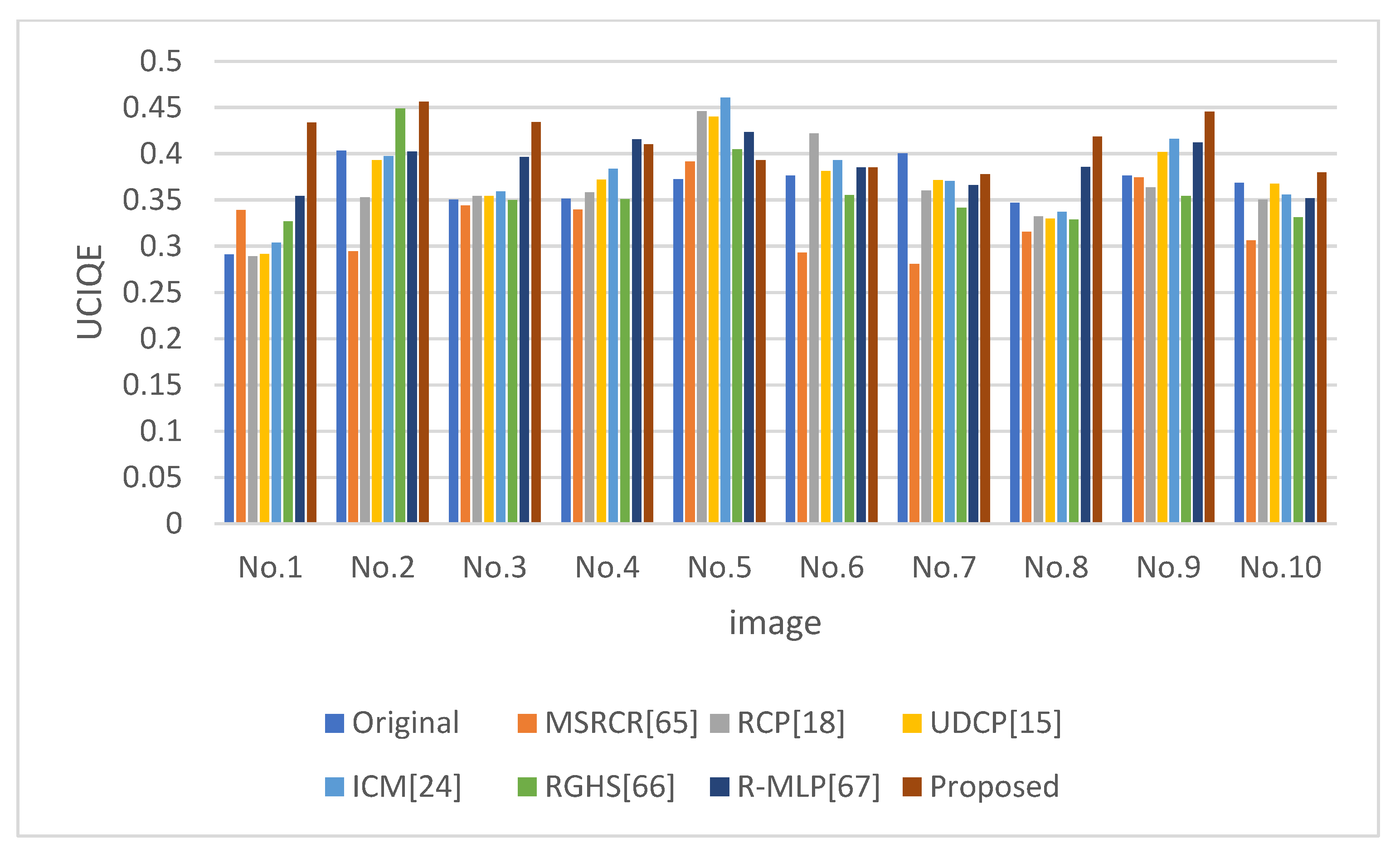
5.3. Quantitative Evaluation

Due to the discrepancy of individual perception, the visual effect of a processed image might be different for a different person. Therefore, quantitative evaluation metrics are necessary. In the study, four commonly used metrics, including root mean square (RMS) contrast, average gradient, underwater color image quality evaluation (UCIQE), and information entropy are used to evaluate the quality of processed underwater images. The RMS contrast reflects the degree of grayscale difference in an image. Average gradient indicates not only the contrast but also the clarity of an image. Comparatively, UCIQE is a more comprehensive metric, since chroma, saturation, and luminance contrast of an image are concerned in this metric. The last metric, information entropy, is a general metric, since it provides the amount of information contained in an image. The four dimensionless metrics are defined as follows. In general, the higher the value of any metric is, the better quality an image has.

The metric of RMS contrast is defined as:

$$\sigma =\sqrt{\frac{1}{M\times N}{\displaystyle \sum _{}{(I(x,y)-\frac{1}{M\times N}{\displaystyle \sum _{}I(x,y)})}^2}},$$

(35)

where M and N are the image width and height; I(x, y) is the pixel gray value at the point (x, y).

The metric of an average gradient is defined as:

$$G=\frac{1}{3}{\displaystyle \sum _{\lambda }\frac{{\displaystyle \sum _{i=1}^M{\displaystyle \sum _{j=1}^N\sqrt{\frac{{\left(\frac{\partial f}{\partial x}\right)}^2+{\left(\frac{\partial f}{\partial y}\right)}^2}{2}}} }}{M\times N}},\lambda \in \left\{r,g,b\right\}.$$

(36)

where $f=f(x,y)$ is the gray value.

The UCIQE metric is defined as:

$$UCIQE=C_1{\sigma }_{\mathrm{c}}+C_{2}co{n}_1+C_3{\mu }_{\mathrm{s}},$$

(37)

where C_i are constants; ${\sigma }_{\mathrm{c}}$ is the standard deviation of chroma; $co{n}_1$ is the brightness contrast; ${\mu }_{\mathrm{s}}$ is the mean saturation.

The metric of information entropy is defined as:

$$Entropy=-{\displaystyle \sum _{i=0}^{N}p(i){\log }_{2}p(i)}.$$

(38)

where i is the gray level with N as the maximum; p(i) is the probability when the pixel value equals i.

By means of the above four metrics,

Table 2. Evaluation of images by RMS contrast.

Image	Original	MSRCR [65]	RCP [18]	UDCP [15]	ICM [24]	RGHS [66]	R-MLP [67]	Proposed
No.1	5.3081	7.4120	6.0984	6.2435	6.7897	10.2875	17.2354	25.4847
No.2	15.1314	14.0953	16.3356	15.5865	15.8495	20.0559	27.5491	36.8800
No.3	10.6724	12.9316	14.3161	14.9913	15.8461	17.4935	28.5648	33.8563
No.4	6.4623	8.2318	7.2596	7.7552	8.7491	7.8784	17.88631	22.0955
No.5	7.8397	10.7915	10.9258	10.9650	13.0286	11.1871	19.5689	22.8650
No.6	5.2668	8.5472	7.8924	7.4822	9.2979	7.8364	14.1568	19.4065
No.7	14.9364	15.6319	16.4253	17.2833	17.6971	16.8500	25.7612	32.9018
No.8	11.2983	14.4708	13.9546	14.4396	15.7776	17.2405	21.6387	29.1649
No.9	10.3155	16.1995	10.2866	10.7759	13.7391	10.7838	17.3652	20.6239
No.10	5.2029	7.4389	5.3538	4.9656	5.4576	5.3483	7.5813	9.4337

,

Table 3. Evaluation of images by average gradient.

Image	Original	MSRCR [65]	RCP [18]	UDCP [15]	ICM [24]	RGHS [66]	R-MLP [67]	Proposed
No.1	2.6423	5.5311	3.8158	3.9434	4.3340	6.9506	8.6724	14.9875
No.2	11.4476	7.9984	12.8501	12.0324	11.6766	14.8117	20.6825	27.1891
No.3	7.2113	9.5290	10.0930	10.4506	9.5695	12.2144	17.3654	23.4287
No.4	4.1082	5.9081	5.0925	5.4805	5.7546	5.5310	8.3642	12.4997
No.5	4.6157	7.6744	7.3803	7.3931	7.4815	7.5037	9.3684	14.1172
No.6	2.7305	5.4254	5.3033	5.0539	4.7643	5.2895	6.8762	10.4021
No.7	10.9880	9.9088	12.5353	13.0484	12.2145	12.7762	19.3653	25.0020
No.8	8.1085	10.2638	10.4221	10.7476	10.4786	12.8594	15.6428	20.8428
No.9	5.5421	6.6848	6.0041	5.6982	6.2871	8.8941	9.5842	11.6465
No.10	2.5368	4.2125	2.4199	2.1152	2.7483	2.4453	4.6843	5.1009

,

Table 4. Evaluation of images by UCIQE.

Image	Original	MSRCR [65]	RCP [18]	UDCP [15]	ICM [24]	RGHS [66]	R-MLP [67]	Proposed
No.1	0.2912	0.3393	0.2889	0.2917	0.3037	0.3267	0.3543	0.4338
No.2	0.4033	0.2944	0.3530	0.3930	0.3973	0.4491	0.4023	0.4562
No.3	0.3504	0.3439	0.3546	0.3545	0.3593	0.3499	0.3964	0.4343
No.4	0.3513	0.3395	0.3581	0.3720	0.3839	0.3509	0.4156	0.4104
No.5	0.3723	0.3914	0.4463	0.4402	0.4608	0.4047	0.4236	0.3933
No.6	0.3765	0.2932	0.4222	0.3815	0.3932	0.3551	0.3851	0.3852
No.7	0.4006	0.2809	0.3603	0.3714	0.3707	0.3415	0.3659	0.3780
No.8	0.3468	0.3158	0.3323	0.3300	0.3371	0.3287	0.3857	0.4188
No.9	0.3766	0.3743	0.3638	0.4021	0.4160	0.3544	0.4123	0.4457
No.10	0.3685	0.3062	0.3502	0.3677	0.3560	0.3312	0.3519	0.3797

and

Table 5. Evaluation of images by information entropy.

Image	Original	MSRCR [65]	RCP [18]	UDCP [15]	ICM [24]	RGHS [66]	R-MLP [67]	Proposed
No.1	5.8674	6.5304	6.4659	6.5056	6.5712	7.4107	7.0365	7.5500
No.2	7.2914	6.9136	7.4504	7.3393	7.3353	7.6421	7.5383	7.3194
No.3	6.6303	6.7505	7.1167	7.0985	7.0791	7.3096	7.6853	7.6887
No.4	7.0890	7.2488	7.4661	7.5578	7.5562	7.5314	7.6695	7.7171
No.5	6.9445	7.4199	7.5348	7.5197	7.5327	7.4902	7.8631	7.6420
No.6	6.4370	7.1931	7.3684	7.2275	7.1261	7.2719	7.3627	7.4410
No.7	7.2052	6.8577	7.3754	7.4174	7.4080	7.3312	7.7261	7.8021
No.8	6.9133	7.0229	7.2435	7.2510	7.2246	7.4810	7.5362	7.6588
No.9	6.7553	6.3295	7.2502	7.0300	6.9953	6.6903	7.5382	7.4103
No.10	7.1588	7.5891	6.9706	7.2512	7.2924	7.4022	7.3696	7.4961

present the evaluation results of ten aforementioned images processed by MSRCR, RCP, UDCP, ICM, RGHS, R-MLP, and the proposed hybrid enhancement method. It is noted that the best metric is shown in bold to distinguish it from the others. Figure 10, Figure 11, Figure 12 and Figure 13 show the visual evaluation metrics.

As can be recognized from the comparison results, in terms of RMS contrast and average gradient, the proposed method obviously and exclusively gains better enhancement than the other algorithms. In terms of UCIQE, the proposed method generally outperforms the others, with three exceptions in image No.4 by R-MLP, in image No.5 by ICM, and in image No.6 by RCP. Similarly, in terms of information entropy, the proposed method generally outperforms the other algorithms, with four exceptions in image No.2 by RGHS, in images No.5 and No.9 by R-MLP, and in image No.10 by MSRCR. Nevertheless, it is noted that in these four exceptions the proposed method still performs well.

To further verify the effectiveness of the proposed enhancement method, the performance of edge detection is evaluated. In the field of image processing, edge detection is important for image classification, target recognition, and feature identification, since the results of detection reflect the quality of an image. Usually, a high-quality image contains more edge information than a low-quality image. In the study, the Canny edge detector is employed. This detector applies a multi-step algorithm to detect a wide range of edges in images. During past decades, it was widely used in various computer vision systems. Figure 14 presents the comparison results of three images by different algorithms. As can be recognized, the proposed enhancement method gains more edge information in images than the other algorithms.

6. Conclusions

In the study, a CNN-based underwater image enhancement method is proposed. The enhancement strategy involves three modules. First, due to the commonly existing color deviation of underwater images, a CNN-based generative adversarial network (GAN) is constructed to achieve a color balance of underwater images. From the ablation experiments, it is confirmed that GAN can effectively diminish the color deviation. However, the processed images are blurred and the contrast is low. To improve the clarity of images, the conventional imaging model is modified to an all-in-one model, in which a comprehensive index is introduced and estimated by a deep CNN. This introduction is to reduce the accumulated errors resulting from the individual estimation of transmittance and background light. The third measure to enhance underwater images is to improve the overall contrast, and increase local details as well, by using a fusion algorithm. To demonstrate the effectiveness of the proposed method, five commonly used algorithms are compared. Comparison is conducted from subjective visual effects and quantitative evaluation. In the quantitative evaluation, several classical evaluation metrics are employed and edge detection is performed. From the comparison results, it can be seen that the proposed method gains better results over the other algorithms. The proposed method can effectively enhance the underwater image quality since it solves the problems of underwater image color degradation, image blur, and low contrast. The enhanced results are more in line with the visual perception of human eyes, conducive to the recognition of human eyes and machines.

Due to the complexity and uncertainty of underwater environments, enhancement of underwater images is challenging and more work needs to be conducted. It is noted that noise was not considered in the study. In the future work, efforts will be devoted to the removal of noises. Moreover, it should be noted that the method proposed in this paper is a combination of three algorithms, which implies it is time-consuming. For some occasions where real-time performance is required, the algorithm proposed is not suitable. Therefore, the improvement of the real-time performance of the algorithm will be studied in the next work. Additionally, it should be noted that the quality measures used in the study do not measure color correctness, and consequently are skewed towards rewarding the oversharpening of images. Such an issue will be studied in future work.

References

1. Singh, H.; Adams, J.; Mindell, D.; Foley, B. Imaging underwater for archaeology. J. Field Archaeol. 2000, 27, 319–328. [Google Scholar]
2. Boudhane, M.; Nsiri, B. Underwater image processing method for fish localization and detection in submarine environment. J. Vis. Commun. Image Represent. 2016, 39, 226–238. [Google Scholar] [CrossRef]
3. Shi, H.; Fang, S.J.; Chong, B.; Qiu, W. An underwater ship fault detection method based on Sonar image processing. J. Phys. Conf. Ser. 2016, 679, 012036. [Google Scholar]
4. Ahn, J.; Yasukawa, S.; Sonoda1, T.T.; Ura, T.; Ishii, K. Enhancement of deep-sea floor images obtained by an underwater vehicle and its evaluation by crab recognition. J. Mar. Sci. Technol. 2017, 22, 758–770. [Google Scholar] [CrossRef]
5. Gu, L.; Song, Q.; Yin, H.; Jia, J. An overview of the underwater search and salvage process based on ROV. Sci. Sin. Inform. 2018, 48, 1137–1151. [Google Scholar] [CrossRef]
6. Watanabe, J.-I.; Shao, Y.; Miura, N. Underwater and airborne monitoring of marine ecosystems and debris. J. Appl. Remote Sens. 2019, 13, 044509. [Google Scholar] [CrossRef]
7. Powar, O.; Wagdarikar, N. A review: Underwater image enhancement using dark channel prior with gamma correction. Int. J. Res. Appl. Sci. Eng. Technol. 2017, 5, 421–426. [Google Scholar] [CrossRef]
8. Zhang, X.; Hu, L. Effects of temperature and salinity on light scattering by water. In Ocean Sensing and Monitoring II; SPIE: Washington, DC, USA, 2010; Volume 7678, pp. 247–252. [Google Scholar]
9. Silver, M. Marine snow: A brief historical sketch. Limnol. Oceanogr. Bull. 2015, 24, 5–10. [Google Scholar] [CrossRef]
10. He, D.; Seet., G. Divergent-beam Lidar imaging in turbid water. Opt. Laser Eng. 2004, 41, 217–231. [Google Scholar] [CrossRef]
11. Ouyang, B.; Dalgleish, F.; Vuorenkoski, A.; Britton, W. Visualization and image enhancement for multistatic underwater laser line scan system using image-based rendering. IEEE J. Ocean. Eng. 2013, 38, 566–580. [Google Scholar] [CrossRef]
12. Jaffe, J. Computer modeling and the design of optimal underwater imaging systems. IEEE J. Ocean. Eng. 1990, 15, 101–111. [Google Scholar] [CrossRef]
13. Trucco, E.; Olmos-Antillon, A. Self-tuning underwater image restoration. IEEE J. Ocean. Eng. 2006, 31, 511–519. [Google Scholar] [CrossRef]
14. Wang, N.; Qi, L.; Dong, J.; Fang, H.; Chen, X.; Yu, H. Two-stage underwater image restoration based on a physical model. In Proceedings of the Eighth International Conference on Graphic and Image Processing (ICGIP 2016), Tokyo, Japan, 29–31 October 2016; p. 10225. [Google Scholar]
15. Wagner, B.; Nascimento, E.R.; Barbosa, W.V.; Campos, M.F.M. Single-shot underwater image restoration: A visual quality-aware method based on light propagation model. J. Vis. Commun. Image Represent. 2018, 55, 363–373. [Google Scholar]
16. Shi, Z.; Feng, Y.; Zhao, M.; Zhang, E.; He, L. Normalized gamma transformation based contrast limited adaptive histogram equalization with color correction for sand-dust image enhancement. IET Image Process. 2020, 14, 747–756. [Google Scholar] [CrossRef]
17. He, K.; Sun, J.; Tang, X. Single image haze removal using dark channel prior. IEEE Trans. Pattern Anal. 2011, 33, 2341–2353. [Google Scholar]
18. Galdran, A.; Pardo, D.; Picón, A.; Alvarez-Gila, A. Automatic red-channel underwater image restoration. J. Vis. Commun. Image Represent. 2015, 26, 132–145. [Google Scholar] [CrossRef]
19. Li, C.; Guo, J.; Wang, B.; Cong, R.; Zhang, Y.; Wang, J. Single underwater image enhancement based on color cast removal and visibility restoration. J. Electron. Imaging 2016, 25, 033012. [Google Scholar] [CrossRef]
20. Tang, Z.; Zhou, B.; Dai, X.; Gu, H. Underwater robot visual enhancements based on the improved DCP algorithm. Robot 2018, 40, 222–230. [Google Scholar]
21. Xie, H.; Peng, G.; Wang, F.; Yang, C. Underwater image restoration based on background light estimation and dark channel prior. Acta Opt. Sin. 2018, 38, 18–27. [Google Scholar]
22. Yu, H.; Li, X.; Lou, Q.; Lei, C.; Liu, Z. Underwater image enhancement based on DCP and depth transmission map. Multimed. Tools Appl. 2020, 79, 20373–20390. [Google Scholar] [CrossRef]
23. Henke, B.; Vahl, M.; Zhou, Z. Removing color cast of underwater images through non-constant color constancy hypothesis. In Proceedings of the 2013 8th International Symposium on Image and Signal Processing and Analysis (ISPA), Trieste, Italy, 4–6 September 2014; pp. 20–24. [Google Scholar]
24. Iqbal, K.; Abdul, S.; Talib, R.; Abdullah, Z. Underwater image enhancement using an integrated colour model. IAENG Int. J. Comput. Sci. 2007, 34, 239–244. [Google Scholar]
25. Guraksin, G.; Deperlioglu, O.; Kose, U. A novel underwater image enhancement approach with wavelet transform supported by differential evolution algorithm. In Nature Inspired Optimization Techniques for Image Processing Applications; Springer: Cham, Switzerland, 2019; pp. 255–278. [Google Scholar]
26. Tang, C.; von Lukas, U.; Vahl, M.; Wang, S.; Wang, Y.; Tan, M. Efficient underwater image and video enhancement based on Retinex. Signal Image Video Process. 2019, 13, 1011–1018. [Google Scholar] [CrossRef]
27. Qiao, X.; Bao, J.; Zhang, H.; Zeng, L.; Li, D. Underwater image quality enhancement of sea cucumbers based on improved histogram equalization and wavelet transform. Inf. Process. Agric. 2017, 4, 206–213. [Google Scholar] [CrossRef]
28. Ghani, A. Image contrast enhancement using an integration of recursive-overlapped contrast limited adaptive histogram specification and dual-image wavelet fusion for the high visibility of deep underwater image. Ocean Eng. 2018, 162, 224–238. [Google Scholar] [CrossRef]
29. Ancuti, C.; Ancuti, C.O.; Haber, T.; Bekaert, P. Enhancing underwater images and videos by fusion. In Proceedings of the 2012 IEEE Conference on Computer Vision and Pattern Recognition, Providence, RI, USA, 16–21 June 2012; pp. 81–88. [Google Scholar]
30. Mohan, S.; Simon, P. Underwater image enhancement based on histogram manipulation and multiscale fusion. Procedia Comput. Sci. 2020, 171, 941–950. [Google Scholar] [CrossRef]
31. Li, C.; Guo, J.; Cong, R.; Pang, Y.; Wang, B. Underwater image enhancement by dehazing with minimum information loss and histogram distribution prior. IEEE Trans. Image Process. 2016, 99, 5664–5677. [Google Scholar] [CrossRef]
32. Xia, W.; Yang, P.; Wang, S.; Xu, B.; Liu, H. Underwater image enhancement based on red channel weighted compensation and gamma correction model. Opto-Electron. Adv. 2018, 1, 13–21. [Google Scholar]
33. Wang, Y.; Yan, Y.; Ding, X.; Fu, X. Underwater Image Enhancement via L2 based Laplacian Pyramid Fusion. In Proceedings of the Oceans 2019 MTS/IEEE Seattle, Washington, DC, USA, 27–31 October 2019; pp. 1–4. [Google Scholar]
34. Luo, W.; Duan, S.; Zheng, J. Underwater image restoration and enhancement based on a fusion algorithm with color balance, contrast optimization and histogram stretching. IEEE Access 2021, 9, 31792–31804. [Google Scholar] [CrossRef]
35. Singh, M.; Vijay, L.; Parvez, F. Visibility enhancement and dehazing: Research contribution challenges and direction. Comput. Sci. Rev. 2022, 44, 00473. [Google Scholar] [CrossRef]
36. Arif, Z.H.; Mahmoud, M.A.; Abdulkareem, K.H.; Mohammed, M.A.; Al-Mhiqani, M.N.; Mutlag, A.A.; Damaševičius, R. Comprehensive review of machine learning (ML) in image defogging: Taxonomy of concepts, scenes, feature extraction, and classification techniques. IET Image Process. 2022, 16, 289–310. [Google Scholar] [CrossRef]
37. Manzo, M.; Simone, P. Voting in transfer learning system for ground-based cloud classification. Mach. Learn. Knowl. Extr. 2021, 3, 542–553. [Google Scholar] [CrossRef]
38. Li, Y.; Lu, H.; Li, J.; Li, X.; Li, Y.; Serikawa, S. Underwater image de-scattering and classification by deep neural network. Comput. Electr. Eng. 2016, 54, 68–77. [Google Scholar] [CrossRef]
39. Perez, J.; Attanasio, A.C.; Nechyporenko, N.; Sanz, P.J. A deep learning approach for underwater image enhancement. In Proceedings of the International Work-Conference on the Interplay between Natural and Artificial Computation, Corunna, Spain, 19–23 June 2017; pp. 183–192. [Google Scholar]
40. Wang, Y.; Zhang, J.; Cao, Y.; Wang, Z. A deep CNN method for underwater image enhancement. In Proceedings of the 2017 IEEE International Conference on Image Processing (ICIP), Beijing, China, 17–20 September 2017; pp. 1382–1386. [Google Scholar]
41. Saeed, A.; Li, C.; Porikli, F. Deep underwater image enhancement. arXiv 2018, arXiv:1807.03528. [Google Scholar]
42. Wang, K.; Hu, Y.; Chen, J.; Wu, X.; Zhao, X.; Li, Y. Underwater image restoration based on a parallel convolutional neural network. Remote Sens. 2019, 11, 1591. [Google Scholar] [CrossRef]
43. Mhala, N.C.; Pais, A.R. A secure visual secret sharing (VSS) scheme with CNN-based image enhancement for underwater images. Vis. Comput. 2020, 37, 2097–2111. [Google Scholar] [CrossRef]
44. Fabbri, C.; Islam, M.J.; Sattar, J. Enhancing underwater imagery using generative adversarial networks. In Proceedings of the 2018 IEEE International Conference on Robotics and Automation (ICRA), Brisbane, Australia, 21–25 May 2018; pp. 7159–7165. [Google Scholar]
45. Li, J.; Skinner, K.A.; Eustice, R.M.; Johnson-Roberson, M. WaterGAN: Unsupervised generative network to enable real-time color correction of monocular underwater images. IEEE Robot. Autom. Lett. 2018, 3, 387–394. [Google Scholar] [CrossRef]
46. Liu, P.; Wang, G.; Qi, H.; Zhang, C.; Zheng, H.; Yu, Z. Underwater image enhancement with a deep residual framework. IEEE Access 2019, 7, 94614–94629. [Google Scholar] [CrossRef]
47. Guo, Y.; Li, H.; Zhuang, P. Underwater image enhancement using a multiscale dense generative adversarial network. IEEE J. Ocean. Eng. 2020, 45, 862–870. [Google Scholar] [CrossRef]
48. Yang, M.; Hu, K.; Du, Y.; Wei, Z.; Sheng, Z.; Hu, J. Underwater image enhancement based on conditional generative adversarial network. Signal Process. Image Commun. 2020, 81, 115723. [Google Scholar] [CrossRef]
49. Zhang, T.; Li, Y.; Takahashi, S. Underwater image enhancement using improved generative adversarial network. Concurr. Comput. Pract. Exp. 2022, 33, e5841. [Google Scholar] [CrossRef]
50. Liu, X.; Gao, Z.; Chen, B.M. IPMGAN: Integrating physical model and generative adversarial network for underwater image enhancement. Neurocomputing 2021, 453, 538–551. [Google Scholar] [CrossRef]
51. Jia, D.; Wei, D.; Socher, R.; Li, L.; Kai, L.; Li, F. ImageNet: A Large-Scale Hierarchical Image Database. In Proceedings of the IEEE Conference on Computer Vision and Pattern Recognition, Miami, FL, USA, 20–21 June 2009; pp. 248–255. [Google Scholar]
52. Islam, M.J.; Xia, Y.; Sattar, J. Fast Underwater Image Enhancement for Improved Visual Perception. IEEE Robot. Autom. Lett. 2020, 5, 3227–3234. [Google Scholar] [CrossRef]
53. Mclean, J.W.; Voss, K.J. Point spread function in ocean water: Comparison between theory and experiment. Appl. Opt. 1991, 30, 2027–2030. [Google Scholar] [CrossRef] [PubMed]
54. Carlevaris-Bianco, N.; Mohan, A.; Eustice, R.M. Initial results in underwater single image dehazing. In Proceedings of the Oceans 2010 Mts/IEEE Seattle, Seattle, WA, USA, 20–23 September 2010; pp. 1–8. [Google Scholar]
55. Wen, H.; Tian, Y.; Huang, T.; Gao, W. Single underwater image enhancement with a new optical model. In Proceedings of the 2013 IEEE International Symposium on Circuits and Systems (ISCAS), Beijing, China, 19–23 May 2013; pp. 753–756. [Google Scholar]
56. Chao, L.; Wang, M. Removal of water scattering. In Proceedings of the 2010 2nd International Conference on Computer Engineering and Technology, Bali Island, Indonesia, 26–29 March 2010; Volume 2, pp. 35–39. [Google Scholar]
57. Chiang, J.Y.; Chen, Y.-C. Underwater image enhancement by wavelength compensation and dehazing. IEEE Trans. Image Process. 2012, 21, 1756–1769. [Google Scholar] [CrossRef] [PubMed]
58. Peng, Y.-T.; Cosman, P.C. Underwater image restoration based on image blurriness and light absorption. IEEE Trans. Image Process. 2017, 26, 1579–1594. [Google Scholar] [CrossRef]
59. Song, W.; Wang, Y.; Huang, D.; Tjondronegoro, D. A rapid scene depth estimation model based on underwater light attenuation prior for underwater image restoration. Adv. Multimed. Inf. Process. 2018, 11164, 678–688. [Google Scholar]
60. Goodfellow, I.; Pouget-Abadie, J.; Mirza, M.; Xu, B.; Warde-Farley, D.; Ozair, S.; Courville, A.; Bengio, Y. Generative adversarial networks. Adv. Neural Inf. Process. Syst. 2014, 3, 2672–2680. [Google Scholar] [CrossRef]
61. Xie, Q.S. Research on the Method of Converting Color Image to Gray Image; Lanzhou University: Lanzhou, China, 2016. [Google Scholar]
62. Wu, X. A Linear Programming Approach for Optimal Contrast-Tone Mapping. IEEE Trans. Image Process. 2011, 20, 1262–1272. [Google Scholar]
63. Silberman, N.; Hoiem, D.; Kohli, P.; Fergus, R. Indoor segmentation and support inference from rgbd images. In European Conference on Computer Vision; Springer: Berlin/Heidelbergpages, Germany, 2012; pp. 746–760. [Google Scholar]
64. Liu, R.; Fan, X.; Zhu, M.; Hou, M.; Luo, Z. Real-World underwater enhancement: Challenges, benchmarks, and solutions under natural light. IEEE Trans. Circuits Syst. Video Technol. 2020, 30, 4861–4875. [Google Scholar] [CrossRef]
65. Rahman, Z.U.; Jobson, D.J.; Woodell, G.A. Retinex Processing for Automatic Image Enhancement. J. Electron. Imaging 2004, 13, 100–110. [Google Scholar]
66. Huang, D.; Yan, W.; Wei, S.; Sequeira, J.; Mavromatis, S. Shallow-water Image Enhancement Using Relative Global Histogram Stretching Based on Adaptive Parameter Acquisition. In Proceedings of the International Conference on Multimedia Modeling, Bangkok, Thailand, 5–7 February 2018; pp. 453–465. [Google Scholar]
67. Zhang, T.T.; Li, Y.; Li, Y.; Li, B.; Lu, H. Underwater image enhancement using Retinex and multilayer perceptron. In Proceedings of the 4th International Symposium on Artificial Intelligence and Robotics, Daegu, Korea, 20–24 August 2019; pp. 1–12. [Google Scholar] [CrossRef]
Figure 1. Typical CNN architecture.
Electronics 11 02537 g001
Figure 2. Underwater image enhancement by UGAN-based color balance, CNN-based dehazing, and contrast improvement.
Electronics 11 02537 g002
Figure 3. Generative adversarial network (GAN).
Electronics 11 02537 g003
Figure 4. The architectures of generative network (a) and discriminative network (b).
Electronics 11 02537 g004aElectronics 11 02537 g004b
Figure 5. Dehazing of underwater images using all-in-one model.
Electronics 11 02537 g005
Figure 6. Framework of CNN structure for K(x).
Electronics 11 02537 g006
Figure 7. Contrast improvement of underwater images.
Electronics 11 02537 g007
Figure 8. Comparison of visual effect by six algorithms.
Electronics 11 02537 g008aElectronics 11 02537 g008b
Figure 9. Ablation experiments. (a) images processed by GAN, the all-in-one model-based CNN, and adaptive contrast enhancement; (b) images processed by GAN and the all-in-one model-based CNN; (c) images processed by GAN; (d) original images.
Electronics 11 02537 g009
Figure 10. Comparison of RMS contrast [15,18,24,65,66,67].
Electronics 11 02537 g010
Figure 11. Comparison of average gradient [15,18,24,65,66,67].
Electronics 11 02537 g011
Figure 12. Comparison of UCIQE [15,18,24,65,66,67].
Electronics 11 02537 g012
Figure 13. Comparison of information entropy [15,18,24,65,66,67].
Electronics 11 02537 g013
Figure 14. Edge detection [15,18,24,65,66,67].
Electronics 11 02537 g014