Optimised Sliding Mode Control of a Hexacopter: Simulation and Experiments

Abstract

Hexacopters are a kind of unmanned aerial vehicle (UAV) with six actuators and six degrees-of-freedom motions. The control of a hexacopter drone is a critical challenge. This paper presents a nonlinear dynamical model for a hexacopter and complete control approaches based on sliding mode control theory. Furthermore, this study proposed an effective control tuning method based on an optimisation algorithm. The controller has been improved by the grey wolf optimisation (GWO) algorithm, an iteration algorithm inspired by the social hierarchy and hunting behaviour of grey wolves. The improvement of the controller has been verified both experimentally and in simulations. The performance of the sub-controller for an attitude angle was tested in a test bench, and the whole flight controller was tested in simulation hexacopters, which are highly manoeuvrable, nonlinear aerial vehicles with six independent rotors and capacity for vertical take-off and landing. This article presents a derivation of the nonlinear dynamical model for a hexacopter, which includes the aerodynamic drag, and inertia counter torques. Flight control based on sliding mode control theory, which generally shows good performance on nonlinear systems, is developed and implemented. Given the need to simultaneously tune controller parameters, two nature inspired optimisation routines (GWO and PSO) are applied and compared for effectiveness in controller tuning. Results indicate that GWO-based tuning produces superior outcomes in terms of controller performance. This is in addition to the fact that PSO parameters require tuning rather than random selection of algorithm parameters. A reduced-order physical prototype is presented for the validation of the tuning routine on the roll/pitch control. The results indicate good agreement between simulation and experimental outcomes, with about 10.4% improvement in the tracking performance of roll DOF when GWO is applied to tune the controller.

1. Introduction

In recent years, multirotor UAVs (commonly known as drones) have become popular and widely used. Compared to traditional helicopters, drones have a simper mechanical structure, which is easier to control [1]. As a result, drones are widely used for aerial filming. They have potential applications in search and rescue operations, environment monitoring, law enforcement, precision agriculture, traffic management, delivery, etc.

The most commonly used drones are quadcopters or quadrotor helicopters. Drones with more rotors, however, have a higher thrust-to-weight ratio and a greater load capacity but generally, higher energy consumption. However, a drone with more rotors, such as a hexacopter, can consume lower energy under certain mass distribution conditions than a quadrotor with the same material and the same motor, as demonstrated in Sun’s research [2]. This study investigates the enhancement of the potential of a hexacopter through the development of an optimised sliding mode control (SMC) model. Although more research has focussed on quadrotors, the core of the flight control structure is similar for both quadrotors and hexacopters.

In order to meet the requirements of remote control and the autonomous flight of a drone, designing a flight controller is a critical task. The study of control usually starts from the PID control theory. The traditional PID control approach can partially meet these requirements. Salih et al. applied the PID control approach for the remote control of a quadcopter. The results show that the controller responds quickly. However, there are obvious oscillations and overshoots [3]. Mustapa et al. applied PID control for the altitude controller of a quadcopter. Altitude control is a relatively simple part of a drone flight controller, which can be addressed by the classic PID approach [4].

Agha [5] and Abidali [6] each studied the PID controller as a baseline controller for solar-powered drones and used other approaches to improve the performance. Bouabdallah’s early work on quadrotor flight control was mainly focused on the backstepping control approach, which was validated in experiments [7]. Bouabdallah also studied the sliding mode control (SMC) approach with Siegwart [7,8,9]. J.A. Ricardo Jr and D.A. Santos studied a smooth second-order SMC for a hexacopter for position and attitude control problems [10]. Moya et al. studied SMC for a drone and confirmed its advantages over PID controllers [11]. In Chiew et al.’s research about altitude and yaw control of a quadcopter, second-order SMC outperformed PD control in all considered performance indicators. [12] Abrougui et al. proposed a robust SMC scheme to stabilise the attitude of a hexacopter during waypoint tracking [13].

Tuning is a critical process of control approaches development; it refers to adjusting the coefficients of the controller to improve performance. Agha, for example, used the Ziegler–Nichols tuning method in the case of PID control, and both Agha and Abidali used fuzzy logic theory to improve the performance of the PID controllers [5,6]. The tuning of SMC has also been studied, for example, Concha et al. developed a tuning algorithm for SMC and applied it into attenuating the structural vibration. [14] Nekoukar and Dehkordi applied fuzzy logic-based theory on a sliding mode controller of a quadcopter, which achieved robust past tracking. [15]

Optimisation algorithms have been widely used in tuning, for example, particle swarm optimisation (PSO) and grey wolf optimisation (GWO). Both approaches involve biomimicry to obtain the optimal solution. They are characterised by the fact that they do not require in-depth knowledge of the system to obtain the optimal solution; just as animals arriving in a new environment can also obtain their prey quickly in some way. So, these approaches have a wide range of applications. Liu et al. applied PSO on SMC for a vector machine [16]; Kumar et al. utilised PSO- and GWO-optimised SMC on frequency regulation. [17] These approaches have also been applied to drones; for example, PSO has previously been used for tuning the PID control of a quadrotor UAV by Noordin et al. [18] and Yin et al. [19]. Qu et al. developed a hybrid GWO algorithm and applied it on the path planning of a drone. [20] However, the study of optimisation-based SMC optimisation for controlling a hexacopter is limited. This study improves the SMC flight controller by using optimisation approaches, such as PSO and GWO.

2. Dynamical Model

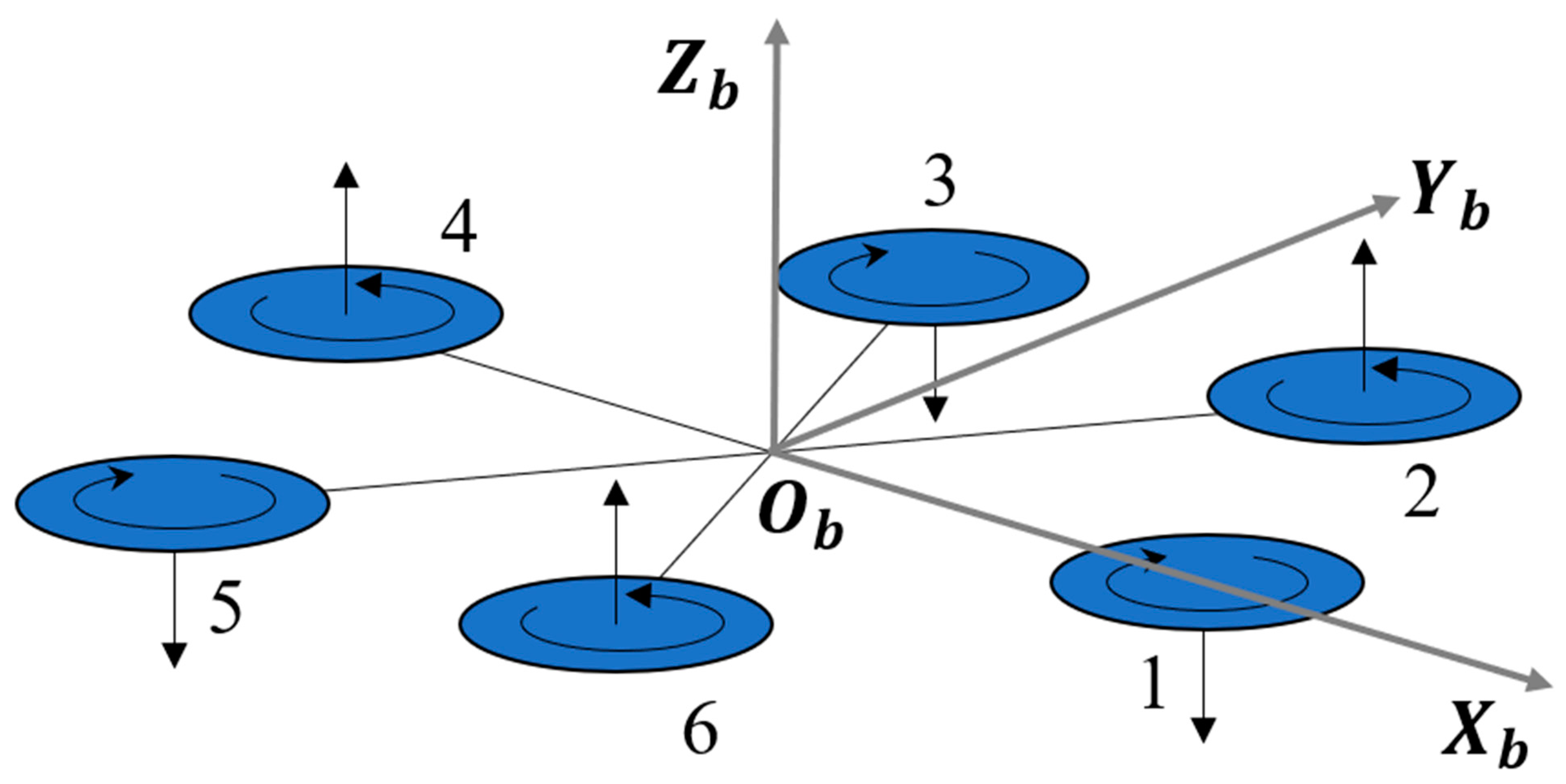
Two coordinate systems are needed to describe the translational and rotational movement of a hexacopter. They are the inertial coordinate (O_iX_iY_iZ_i), based on earth, and the body-fixed coordinate (O_bX_bY_bZ_b) attached to the centre of mass of the drone. For a hexacopter, X_b-axis is on a strip, Y_b-axis is on an angle bisector of two strips, and Z_b-axis is defined by the right-hand rule, as demonstrated in Figure 1. The position of the drone is expressed by vector r in inertial coordinate:

$$\begin{array}{c}\mathit{r}={\left[ \begin{array}{ccc}x& y& z\end{array}\right]}^{\mathit{T}}\end{array}$$

(1)

Moreover, the velocity of the drone is expressed in body-fixed coordinate:

$$\begin{array}{c}\mathit{V}={\left[\begin{array}{ccc}{v}_x& v_y& v_z\end{array} \right]}^{\mathit{T}}\end{array}$$

(2)

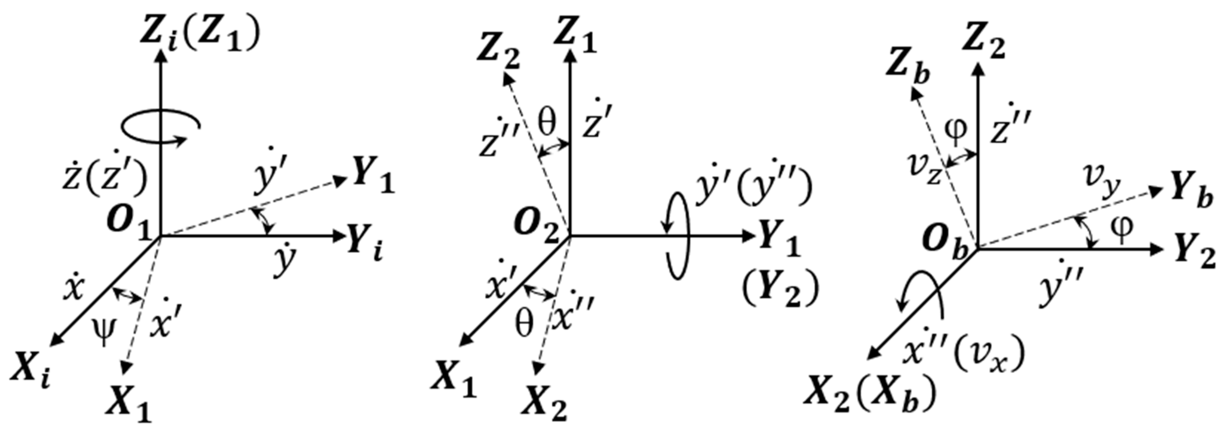
The attitude of the drone is described by Euler angles $\phi \theta \psi$, which expresses roll, pitch, and yaw angles, respectively. In addition, the transformation between inertial and body-fixed coordinates depends on the attitude angles. The two coordinates are coincident initially, and the drone rotates around the z, y, and x axes, as shown in Figure 2. O_{1 × 1}Y₁Z₁ and O₂X₂Y₂Z₂ are two intermediate coordinates after the first and second rotation; accordingly,$\dot{ {\mathit{r}}_{\mathbf{1}}}={\left[\begin{array}{ccc}\dot{x^{\prime }}& \dot{y^{\prime }}& \dot{z^{\prime }}\end{array}\right]}^{\mathit{T}}$ and $\dot{ {\mathit{r}}_{\mathbf{2}}}={\left[\begin{array}{ccc}\dot{x^{″}}& \dot{y^{″}}& \dot{z^{″}}\end{array}\right]}^{\mathit{T}}$ are the intermediate velocity vectors. The mutual orientation of the coordinates is described by the rotation matrix $R$ [21].

$$\begin{array}{c}\mathit{R}=\left[\begin{array}{ccc}cos\theta cos\psi & sin\phi sin\theta cos\psi -cos\phi sin\psi & cos\phi sin\theta cos\psi +sin\phi sin\psi \\ cos\theta sin\psi & sin\phi sin\theta sin\psi +cos\phi cos\psi & cos\phi sin\theta sin\psi -sin\phi cos\psi \\ -sin\theta & sin\phi cos\theta & cos\phi cos\theta \end{array}\right]\end{array}$$

(3)

The transformation of velocities between the body-fixed and inertial frames is given as:

$$\begin{array}{c}\dot{\mathit{r}}=\mathit{R}\mathit{V}\end{array}$$

(4)

The same angular velocity is expressed differently in different coordinate systems. The vector ω denotes the angular speed of the drone in body-fixed coordinates where $p$, $q$, and $r$ are the angular velocities of hexacopter in the body frame; the vector $\mathit{q}$ is the attitude vector in the earth-fixed frame.

$$\begin{array}{c}\mathit{\omega }={\left[\begin{array}{ccc}p& q& r\end{array} \right]}^{\mathit{T}}\end{array}$$

(5)

$$\begin{array}{c}\mathit{q}={\left[\begin{array}{ccc}\phi & \theta & \psi \end{array} \right]}^{\mathit{T}}\end{array}$$

(6)

The transformation matrix for the angular speed is as follows:

$$\begin{array}{c}{\mathit{R}}_{\mathit{A}}=\left[\begin{array}{ccc}1& 0& -\mathit{sin}\theta \\ 0& \mathit{cos}\phi & \mathit{cos}\theta \mathit{sin}\phi \\ 0& -\mathit{sin}\phi & \mathit{cos}\theta \mathit{cos}\phi \end{array}\right]\end{array}$$

(7)

The transformation of the angular speed is:

$$\begin{array}{c}\mathit{\omega }={\mathit{R}}_{\mathit{A}}\dot{\mathit{q}}\end{array}$$

(8)

Equation (9) is the Newton–Euler equation of motion, which describe the equilibrium of forces of a drone in body coordinate:

$$\left[\begin{array}{c}\mathit{F}\\ \mathit{N}\end{array}\right]=\left[\begin{array}{cc}m{\mathit{I}}_{\mathit{3}}& 0\\ 0& M\end{array}\right]\left[\begin{array}{c}\dot{\mathit{V}}\\ \dot{\mathit{\omega }}\end{array}\right]+\left[\begin{array}{c}\mathit{\omega }\times m\mathit{V}\\ \mathit{\omega }\times M\mathit{\omega }\end{array}\right]$$

(9)

where F is the force vector and N is the torque vector, I₃ is a 3 × 3 identity matrix, and M is the inertia matrix:

$$\begin{array}{c}\mathit{M}=\left[\begin{array}{ccc}{J}_x& 0& 0\\ 0& J_y& 0\\ 0& 0& J_z\end{array}\right] \end{array}$$

(10)

The force is determined by the gravity of the drone and the thrust generated by the rotors, the aerodynamic resistance. The equation of force with transformation can be expressed as Equation (11):

$$\mathit{F}=\left[\begin{array}{c}0\\ 0\\ T\end{array}\right]+{\mathit{R}}^{-1}\left[\begin{array}{c}0\\ 0\\ -mg\end{array}\right]+{\mathit{R}}^{-1}\left[\begin{array}{c}{D}_x\\ D_y\\ D_z+L\end{array}\right]$$

(11)

where $m$ is the mass of the drone, $g$ is gravitational acceleration, and $T$ is the total thrust generated by the propellers.

$$\begin{array}{c}T=b\left({\Omega }_1^2+{\Omega }_2^2+{\Omega }_3^2+{\Omega }_4^2+{\Omega }_5^2+{\Omega }_6^2\right)\end{array}$$

(12)

In Equation (12), $b$ is the thrust coefficient, and ${\Omega }_1$ to ${\Omega }_6$ are the angular speeds of the corresponding propellers.

The aerodynamic resistance of the drone cannot be ignored. The direction of the drag is opposite to the direction of the movement, $D_x$, $D_y,$ and $D_z$are the aerodynamic resistances or drags in x, y, and z direction. [22,23]

In Equation (13), $\rho$ is the air density; $C_{Dx},C_{Dy } and C_{Dz}$ are the drag coefficients, which are dimensionless numbers, depending on the angle of attack (AOA).$C_{Lx}, C_{Ly}$ are dimensionless lift coefficients dependent on the AOA; A is the area of the drone in contact with the air when flying vertically upwards.

$$\begin{array}{c}\begin{array}{c}\{\begin{array}{c}{D}_x=-\frac{1}{2}\rho A{C}_{Dx}\dot{x}\left|\dot{x}\right|\\ D_y=-\frac{1}{2}\rho A{C}_{Dy}\dot{y}\left|\dot{y}\right|\\ D_z=-\frac{1}{2}\rho A{C}_{Dz}\dot{z}\left|\dot{z}\right|\end{array}\\ L=-\frac{1}{2}\rho A\left(C_{Lx}{\dot{x}}^2+C_{Ly}{\dot{y}}^2\right)\end{array}\end{array}$$

(13)

The torque vector $\mathit{N}$:

$$\begin{array}{c}\mathit{N}={\left[\begin{array}{ccc}{N}_x& N_y& N_z\end{array}\right]}^T={\mathit{\tau }}_{\mathit{T}}+{\mathit{\tau }}_{{\mathit{P}}_{\mathit{G}}\mathit{y}\mathit{r}\mathit{o}}+{\mathit{\tau }}_{\mathit{c}\mathit{o}\mathit{u}\mathit{n}\mathit{t}\mathit{e}\mathit{r}}+{\mathit{\tau }}_{\mathit{d}\mathit{r}\mathit{a}\mathit{g}}\end{array}$$

(14)

where ${\mathit{\tau }}_{\mathit{T}}$ is the torque produced by the propellers; ${\mathit{\tau }}_{{\mathit{P}}_{\mathit{G}}\mathit{y}\mathit{r}\mathit{o}}$ is the propeller gyroscopic torque, ${\mathit{\tau }}_{\mathit{c}\mathit{o}\mathit{u}\mathit{n}\mathit{t}\mathit{e}\mathit{r}}$ is the inertial counter-torque; ${\mathit{\tau }}_{\mathit{d}\mathit{r}\mathit{a}\mathit{g}}$ is the torque due to the aerodynamic drag.

For a hexacopter, the torque produced by the propeller is [24,25]:

$$\begin{array}{c}\{\begin{array}{c}\begin{array}{c}{\tau }_{Tx}=\frac{\sqrt{3}}{2}bl\left({\Omega }_5^2+{\Omega }_6^2-{\Omega }_2^2-{\Omega }_3^2\right)\\ {\tau }_{Ty}=bl\left(-{\Omega }_1^2-\frac{1}{2}{\Omega }_2^2+\frac{1}{2}{\Omega }_3^2+{\Omega }_4^2+\frac{1}{2}{\Omega }_5^2-\frac{1}{2}{\Omega }_6^2\right)\\ {\tau }_{Dz}=d\left({\Omega }_1^2+{\Omega }_3^2+{\Omega }_5^2-{\Omega }_2^2-{\Omega }_4^2-{\Omega }_6^2\right)\end{array}\\ \end{array}\end{array}$$

(15)

where $b$ is the thrust factor, $d$ is the drag torque constant, and $l$is the arm length; ${\tau }_{Tx}$ and ${\tau }_{Ty}$ are the torque due to thrust about x-axis on body-fixed frame; ${\tau }_{Dz}$ is the torque about the z-axis, which is dominated by the torque from the drag of the blade.

The propeller gyroscopic effect results from a change of angular momentum of propellers due to the rotation of the hexacopter. It is given by the cross-product of the angular velocity of the hexacopter and the angular momentum of a propeller. The expression is:

$$\begin{array}{c}{\mathit{\tau }}_{{\mathit{P}}_{\mathit{G}\mathit{y}\mathit{r}\mathit{o}}}=\left[\begin{array}{c}-J_{r}q\left({\Omega }_1-{\Omega }_2+{\Omega }_3-{\Omega }_4+{\Omega }_5-{\Omega }_6\right)\\ J_{r}p\left({\Omega }_1-{\Omega }_2+{\Omega }_3-{\Omega }_4+{\Omega }_5-{\Omega }_6\right)\\ 0\end{array}\right]\end{array}$$

(16)

where $J_r$ is the moment of inertia of the rotor (a propeller and a motor).

The inertial counter-torque is the torque required to balance the torque of rotors. The torque is given by the product of the rotor moment of inertia and angular acceleration. Applying the rotation form of Newton’s third law; the counter torques are numerically equal to the rotors torques but in opposite directions. The counter-torque only appears on the z-axis (of the body-fixed frame):

$$\begin{array}{c}{\mathit{\tau }}_{\mathit{c}\mathit{o}\mathit{u}\mathit{n}\mathit{t}\mathit{e}\mathit{r}}=\left[\begin{array}{c}0\\ 0\\ J_r\left({\alpha }_1-{\alpha }_2+{\alpha }_3-{\alpha }_4+{\alpha }_5-{\alpha }_6\right)\end{array}\right]\end{array}$$

(17)

where ${\alpha }_1$ to ${\alpha }_6$ are the angular accelerations of the corresponding propellers.

The drone is also affected by aerodynamics during its rotation. The expression of the torque caused by aerodynamics is:

$$\begin{array}{c}{\mathit{\tau }}_{\mathit{d}\mathit{r}\mathit{a}\mathit{g}}=\left[\begin{array}{c}-C_{Tx}p\left|p\right|\\ -C_{Ty}q\left|q\right|\\ -C_{Tz}r\left|r\right|\end{array}\right]\end{array}$$

(18)

$C_{Tx}$,$C_{Ty}$, and $C_{Tz}$are the drag torque coefficients.

According to Newton–Euler Equation, the acceleration and angular acceleration of the drone in body-fixed coordinate can be calculated with the following equation:

$$\begin{array}{c}\{\begin{array}{c}\dot{\mathit{V}}=\frac{1}{m}\mathit{F}-\mathit{\omega }\times \mathit{V}\\ \dot{\mathit{\omega }}={\mathit{M}}^{-1}\mathit{N}-\mathit{\omega }\times \mathit{\omega }\end{array}\end{array}$$

(19)

The drone’s velocity can be calculated by integrating the acceleration and then transforming the velocity to inertial coordinate by Equations (3) and (4). Likewise, the position can be calculated by integrating the velocity. Similarly, the attitude angle can be calculated by two integrations and one transformation.

3. Control of Hexacopter

The objective of the control is to make the drone fly autonomously following a desired trajectory. The desired trajectory includes the desired position (x, y, z) and the desired yaw angle. The pitch and roll angles are supposed to be small, but they control the position. A state vector is defined [11]:

$$\begin{array}{c}\mathit{x}={\left[x_1 x_2 x_3 x_4 x_5 x_6 x_7 x_8 x_9 x_{10} x_{11} x_{12}\right]}^{\mathit{T}}={\left[\phi \dot{\phi } \theta \dot{\theta } \psi \dot{\psi } z \dot{z} x \dot{x} y \dot{y}\right]}^{\mathit{T}}\end{array}$$

(20)

The 12-state variables are the position in the inertial axis, attitude angles, and their time derivatives (or speed). The 12 state variables correspond to six degrees of freedom. The flight controller can be divided into six sub-controllers, corresponding to the state variables or degrees of freedom. The rotation sub-controllers are roll sub-controller, pitch sub-controller, and yaw sub-controller; the position sub-controllers are z (altitude) sub-controller, x sub-controller, and y sub-controller.

The state of the drone is determined by the thrust and torque provided by the rotors, the control vector of the hexacopter is defined as:

$$\begin{array}{c}\mathit{U}={\left[U_1 U_2 U_{3 }{U}_4 \right]}^T={\left[T N_x N_y N_z\right]}^T\end{array}$$

(21)

After simplification, the dynamical model for the flight controller, the time derivative of the state vector is:

$$\begin{array}{c}\dot{\mathit{x}}=f\left(\mathit{x},\mathit{U}\right)=\left(\begin{array}{c}{x}_2\\ a_1{x}_4{x}_6+b_1{U}_2+b_1{c}_1{x}_2\left|x_2\right|\\ x_4\\ a_2{x}_2{x}_6+b_2{U}_3+b_2{c}_2{x}_4\left|x_4\right|\\ x_6\\ a_3{x}_2{x}_4+b_3{U}_4+b_3{c}_3{x}_6\left|x_6\right|\\ x_8\\ \frac{1}{m}\mathit{cos}{x}_3\mathit{cos}{x}_1{U}_1-g+\frac{1}{m}{c}_4{x}_8\left|x_8\right|+\frac{1}{m}\left(c_5{x}_{10}{}^2+c_6{x}_{12}{}^2\right)\\ x_{10}\\ \frac{1}{m}{u}_x{U}_1+\frac{1}{m}{c}_7{x}_{10}\left|x_{10}\right|\\ x_{12}\\ \frac{1}{m}{u}_y{U}_1+\frac{1}{m}{c}_8{x}_{12}\left|x_{12}\right|\end{array}\right)\end{array}$$

(22)

With

$$\begin{array}{r}{c}_1=-C_{Tx} \\ c_2=-C_{Ty} \\ c_3=-C_{Tz} \\ a_1=\left(J_y-J_z\right)/J_x\hspace{1em}{b}_1=\frac{1}{J_x}\hspace{1em}{c}_4=-\frac{\rho A{C}_{Dz}}{2}\\ a_2=\left(J_z-J_x\right)/J_y\hspace{1em}{b}_2=\frac{1}{J_y}\hspace{1em}{c}_5=-\frac{\rho C_{Lx}A}{2}\\ a_3=\left(J_x-J_y\right)/J_z\hspace{1em}{b}_3=\frac{1}{J_z}\hspace{1em}{c}_6=-\frac{\rho C_{Ly}A}{2}\\ c_7=-\frac{\rho A{C}_{Dx}}{2}\\ c_8=-\frac{\rho A{C}_{Dy}}{2}\\ u_x=\mathit{cos}{x}_5\mathit{sin}{x}_3\mathit{cos}{x}_1+\mathit{sin}{x}_5\mathit{sin}{x}_1 \\ u_y=\mathit{sin}{x}_5\mathit{sin}{x}_3\mathit{cos}{x}_1-\mathit{cos}{x}_5\mathit{sin}{x}_1 \end{array}$$

(23)

The propeller gyro effect and inertial counter-torque are neglected in this equation. $U_2$ is the control variable of roll sub-controller; $U_3$ is for pitch sub-controller; $U_4$ is for yaw sub-controller. $u_x$ and $u_y$ are an expansion of the control variables and are determined by the attitude angles and $U_1.$ They are the control variables of x and y sub-controllers. In addition, conversely, the commanded pitch and roll angle (x_1c, x_3c in the form of state variables) can be calculated by the control variables $u_x$ and $u_y$. When the pitch and roll angles are small,

$$\begin{array}{c} \begin{array}{c}{x}_{1c}=u_x\mathit{sin}{x}_5-u_y\mathit{cos}{x}_5\\ x_{3c}=u_x\mathit{cos}{x}_5+u_y\mathit{sin}{x}_5\end{array}\end{array}$$

(24)

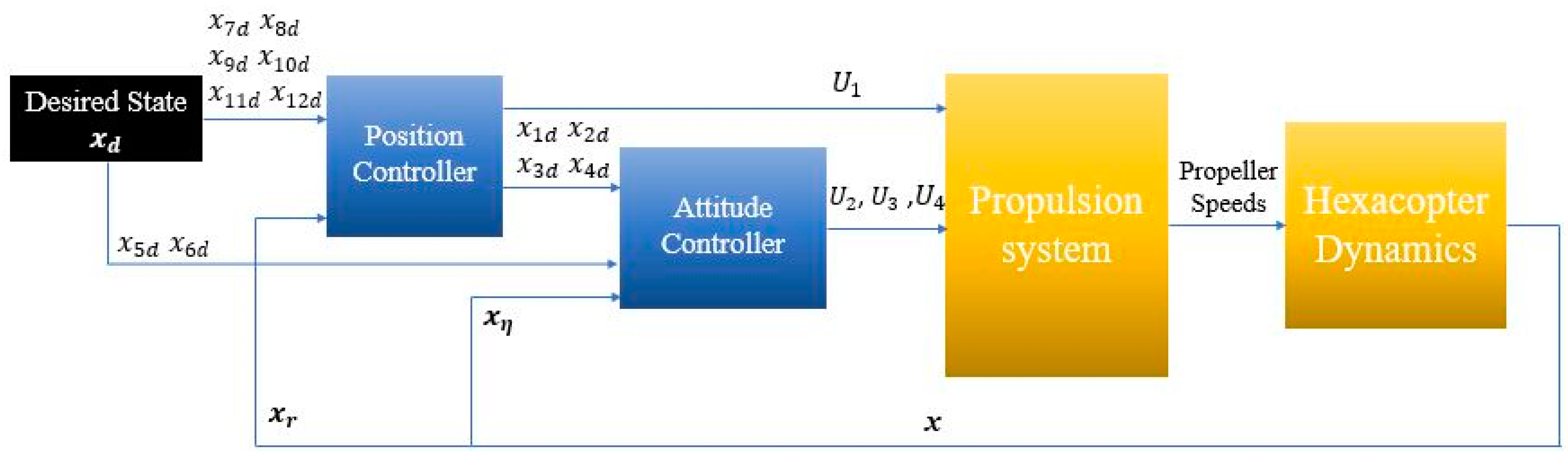
The flight control scheme for a hexacopter is indicated in Figure 3. The input variables are the desired position and yaw angle. First, input the desired position to the position sub-controllers to get the commanded control variable $U_1$ and commanded pitch and roll angles. Then, input the desired yaw angle and commanded pitch and roll angles to the rotation sub-controllers to get the control variables $U_2$, $U_3,$ and $U_4$. The control variables are inputted into the system. The system estimates the actual position and attitude and then feeds back to the sub-controllers.

The control strategy applied in the position and rotation sub-controllers is the sliding mode control approach. It is an iterative method based on Lyapunov stability theory. A sliding surface is designed to drive the state space, and the controller makes the state space reach the sliding surface. When the sliding surface is reached, the controller keeps the state on the neighbourhood of the sliding surface [26]. For a second-order system, such as the roll sub-controller:

$$\begin{array}{c}\{\begin{array}{c}\dot{x_1}=x_2\\ \dot{x_2}=f\left(x_1,x_2\right)+h\left(x_1,x_2\right)U_2\end{array} \end{array}$$

(25)

Define the setpoint x_1d and the error $z_1$:

$$\begin{array}{c}{z}_1=x_{1d}-x_1\end{array}$$

(26)

The sliding surface is defined as follows:

$$\begin{array}{c}{s}_1\left(t\right)=\left\{\left(x_1,x_2\right)|s_1\left(x_1,x_2,t\right)=0\right\}\end{array}$$

(27)

With $s_1\left(x_1,x_2,t\right)$ defined by

$$\begin{array}{c}{s}_1\left(x_1,x_2,t\right)=\left(\frac{d}{dt}+m_1\right)z_1\left(t\right), m_1>0\end{array}$$

(28)

where $m_1$ is a positive constant.

$$\begin{array}{c}{s}_1=\dot{x_{1d}}-x_2+m_1{z}_1\end{array}$$

(29)

To make the state approach, the sliding mode is equivalent with stabilising $s$ to zero, a positive definite Lyapunov candidate function for s is defined as:

$$\begin{array}{c}V\left(s_1\right)=\frac{1}{2}{s}_1{}^2\end{array}$$

(30)

Differentiating:

$$\begin{array}{c}\dot{s_1}=\ddot{x_{1d}}-\left(f\left(x_1,x_2\right)+h\left(x_1,x_2\right)U_2\right)+m_1\left(s_1-m_1{z}_1\right)\end{array}$$

(31)

Define

$$\begin{array}{c} U_2{}^{*}=\frac{1}{h\left(x_1,x_2\right)}\left(\ddot{x_{1d}}+m_1\left(s_1-m_1{z}_1\right)-f\left(x_1,x_2\right)\right)\end{array}$$

(32)

Then, if $U_2=U_2{}^{*}$, $\dot{s_1}=0$ for all time. Following the exponential reaching law:

$$\begin{array}{c} \dot{s_1}=-n_{1}sgn\left(s_1\right)-n_2{s}_1,with U_2=U_2{}^{*}+\frac{1}{h\left(x_1,x_2\right)}\left(n_{1}sgn\left(s_1\right)+n_2{s}_1\right)\end{array}$$

(33)

$$\begin{array}{c} \dot{V}\left(s_1\right)=s_1\dot{s_1}=-n_1\left|s_1\right|-n_2{s}_1{}^2\end{array}$$

(34)

where $n_1$ and $n_2$ are positive constants, the three coefficients of one sliding mode controller. In addition, $\dot{V}\left(s\right)$ is a negative definite function. Apply this control approach to a hexacopter with Equation (22), following the exponential law, the rotation sub-controllers:

$$\begin{array}{c}\{\begin{array}{c}{U}_2=\frac{1}{b_1}\left(\ddot{x_{1d}}+m_1\left(s_1-m_1{z}_1\right)-a_1{x}_4{x}_6-c_1{x}_2\left|x_2\right|+n_{1}sgn\left(s_1\right)+n_2{s}_1\right)\\ U_3=\frac{1}{b_2}\left(\ddot{x_{3d}}+m_2\left(s_2-m_2{z}_3\right)-a_2{x}_3{x}_6-c_2{x}_4\left|x_4\right|+n_{3}sgn\left(s_2\right)+n_4{s}_2\right)\\ U_4=\frac{1}{b_3}\left(\ddot{x_{5d}}+m_3\left(s_3-m_3{z}_5\right)-a_3{x}_2{x}_4-c_3{x}_6\left|x_6\right|+n_{5}sgn\left(s_3\right)+n_6{s}_3\right)\end{array}\end{array}$$

(35)

With

$$\begin{array}{c}\{\begin{array}{c}{s}_1=\dot{x_{1d}}-x_2+m_1{z}_1\\ s_2=\dot{x_{3d}}-x_4+m_2{z}_3\\ s_3=\dot{x_{5d}}-x_6+m_3{z}_5\end{array}\end{array}$$

(36)

And the position sub-controllers:

$$\begin{array}{c}\{\begin{array}{c}{U}_1=\frac{m}{\mathit{cos}\left(x_1\right)\mathit{cos}\left(x_3\right)}\left(\ddot{x_{7d}}+g+m_4\left(s_4-m_4{z}_7\right)-n_{7}sgn\left(s_4\right)+n_8{s}_4-\frac{1}{m}{c}_4{x}_8\left|x_8\right|-\frac{c_5}{m}{x}_{10}{}^2-\frac{c_5}{m}{x}_{12}{}^2\right)\\ u_x=\frac{m}{U_1}\left(\ddot{x_{9d}}-m_5\left(s_5-m_5{z}_9\right)-n_{9}sgn\left(s_5\right)+n_{10}{s}_5-\frac{1}{m}{c}_7{x}_{10}\left|x_{10}\right|\right)\\ u_x=\frac{m}{U_1}\left(\ddot{x_{11d}}-m_6\left(s_6-m_6{z}_{11}\right)-n_{11}sgn\left(s_6\right)+n_{12}{s}_6-\frac{1}{m}{c}_7{x}_{12}\left|x_{12}\right|\right)\end{array}\end{array}$$

(37)

With

$$\begin{array}{c} \{\begin{array}{c}{s}_4=\dot{x_{7d}}-x_8+m_4{z}_7\\ s_5=\dot{x_{9d}}-x_{10}+m_5{z}_9\\ s_6=\dot{x_{11d}}-x_{12}+m_6{z}_{11}\end{array} \end{array}$$

(38)

$z_1$ to $z_{11}$ are the difference between the desired value and real value or error. $m_1$ to $m_6$ and $n_1$ to $n_{12}$ are the control coefficients. In the sliding mode flight controller of the drone, each sub-controller has three coefficients; there are 6 sub-controllers with 18 coefficients. These coefficients have been tuned based on previous experience, the requirements for an autonomous flight can be achieved in this way. However, further improvements can be made by means of optimisation.

4. Optimisation

PSO and GWO have been used to optimise the controllers by tuning the coefficients in this study. Both of these optimisation approaches are derived from biomimicry. PSO is inspired by the social behaviour and dynamical movements with the communication applicable in insects, birds, and fish; GWO is inspired by grey wolves’ social hierarchy and hunting process.

In PSO, all particles are in search of an optimal position. This position is unknown, but it is possible to compare which particle is in a better position. Each particle decides where to move next based on the best position it has experienced and the best position of all the particles [18].

$$\begin{array}{c}\{\begin{array}{c}W\left(t_i+1\right)=w_{0}W\left(t_i\right)+w_1{r}_1\left(P\left(t_i\right)-X\left(t_i\right)\right)+w_2{r}_2\left(G\left(t_i\right)-X\left(t_i\right)\right)\\ X\left(t_i+1\right)=X\left(t_i\right)+W\left(t_i+1\right)\end{array} \end{array}$$

(39)

Equation (39) expresses the direction and position of a particle in the next iteration. $t_i$ is the iteration number, $W$ is the direction, and X is the position. P is the best position reached by the particle, and G is the best position reached by the swarm. $r_1$ and $r_2$ are random numbers between 0 and 1; $w_{ 0},$ $w_1,$ and $w_2$ are positive constants as the coefficients. $w_0$ is usually equal to 1 and $w_1+w_2=4$.

In GWO, four groups are defined in the algorithm to simulate the social hierarchy of grey wolves [27]:

• Alpha (α)—the leaders, called alpha, are responsible for decision-making, such as hunting, sleeping place, time to wake, etc.
• Beta (β)—this is the second level. They are the subordinate wolves, and they help the alpha wolves with decision making.
• Delta (δ)—like beta wolves, they must submit to alpha and beta wolves but dominate the other wolves.
• Omega (ω)—the followers.

During the hunting process, the exact location of the prey is unknown. Therefore, the alpha, beta, and delta wolves have more experience and knowledge about hunting to estimate the prey’s position more accurately. The hunting is guided by alpha, beta, and delta; the omega wolves are followers.

The following equations represent the mathematical model of the hunting behaviour:

$$\begin{array}{c}\{\begin{array}{c}{D}_{\alpha }=\left|C_1{X}_{\alpha }\left(t_i\right)-X\left(t_i\right)\right|\\ D_{\beta }=\left|C_2{X}_{\beta }\left(t_i\right)-X\left(t_i\right)\right|\\ D_{\delta }=\left|C_3{X}_{\delta }\left(t_i\right)-X\left(t_i\right)\right|\end{array}\end{array}$$

(40)

In Equation (40), $t_i$ is the current iteration. Thus, X_α, X_β, and X_δ are the three best positions or the positions of alpha, beta, and delta wolves. X is the position of any wolf in the group; C₁, C₂, and C₃ are random numbers.

$$\begin{array}{c}\{\begin{array}{c}{X}_1=X_{\alpha }-A_1{D}_{\alpha }\\ X_2=X_{\beta }-A_2{D}_{\beta }\\ X_3=X_{\delta }-A_3{D}_{\delta }\\ X\left(t_i+1\right)=\frac{X_1+X_2+X_3}{3}\end{array}\end{array}$$

(41)

In Equation (41), $A_1$, $A_2$, and $A_3$ are adaptive numbers; these two equations define how the wolf moves with the guide of the leaders. The random numbers and adaptive numbers are defined with

$$\begin{array}{c}\{\begin{array}{c}{C}_{1,2,3}=2r_1\\ A_{1,2,3}=2a{r}_2-a\\ a=2-2\left(t_i/max\right)\end{array} \end{array}$$

(42)

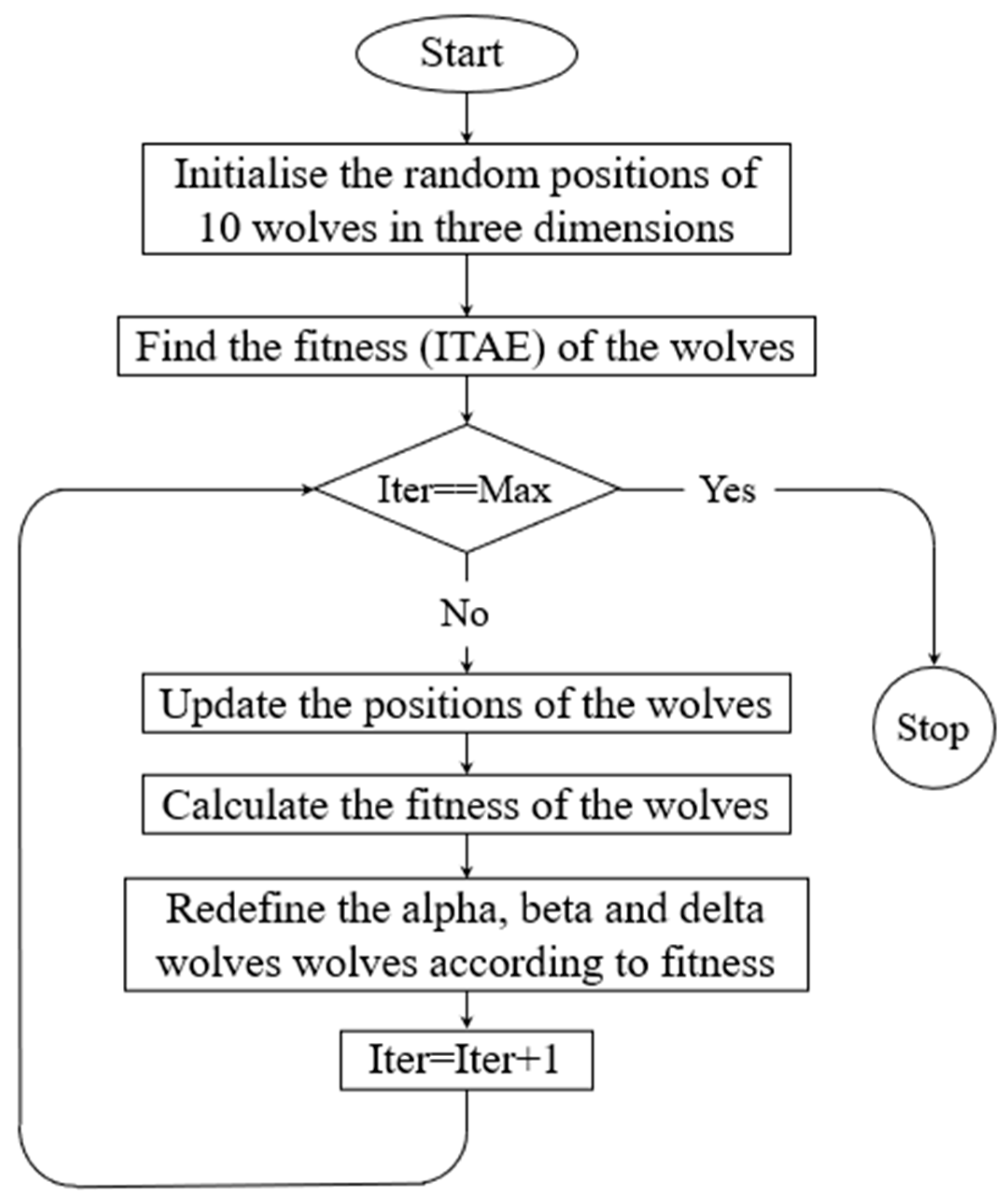
where $r_1$ and $r_2$ are random numbers between 0 and 1, max is the number of iterations. The process of the GWO algorithm is indicated in Figure 4. The three groups of wolves with the highest fitness are alpha, beta, and delta wolves. The position and identity of the wolves are updated in each loop. The system then proceeds to the next iteration (Iter = Iter + 1) until the maximum number of iterations is reached (Iter == max).

At first, the roll sub-controller was used to test the performance of the optimisation algorithms. The 30 degrees step response tested the sets of coefficients of the roll sub-controller. The optimal coefficients are unknown during the optimisation of a sliding mode controller. A total of 10 sets of coefficients are generated randomly, such as ten particles or wolves. The integral of time multiplied absolute error (ITAE, Equation (43)) measured in simulation has been taken as the objective function.

$$\begin{array}{c} \mathrm{ITAE}={\int }_0^{\infty }t\left|e\left(t\right)\right|dt \end{array}$$

(43)

where $e\left(t\right)$ represents the error at a certain operation time.

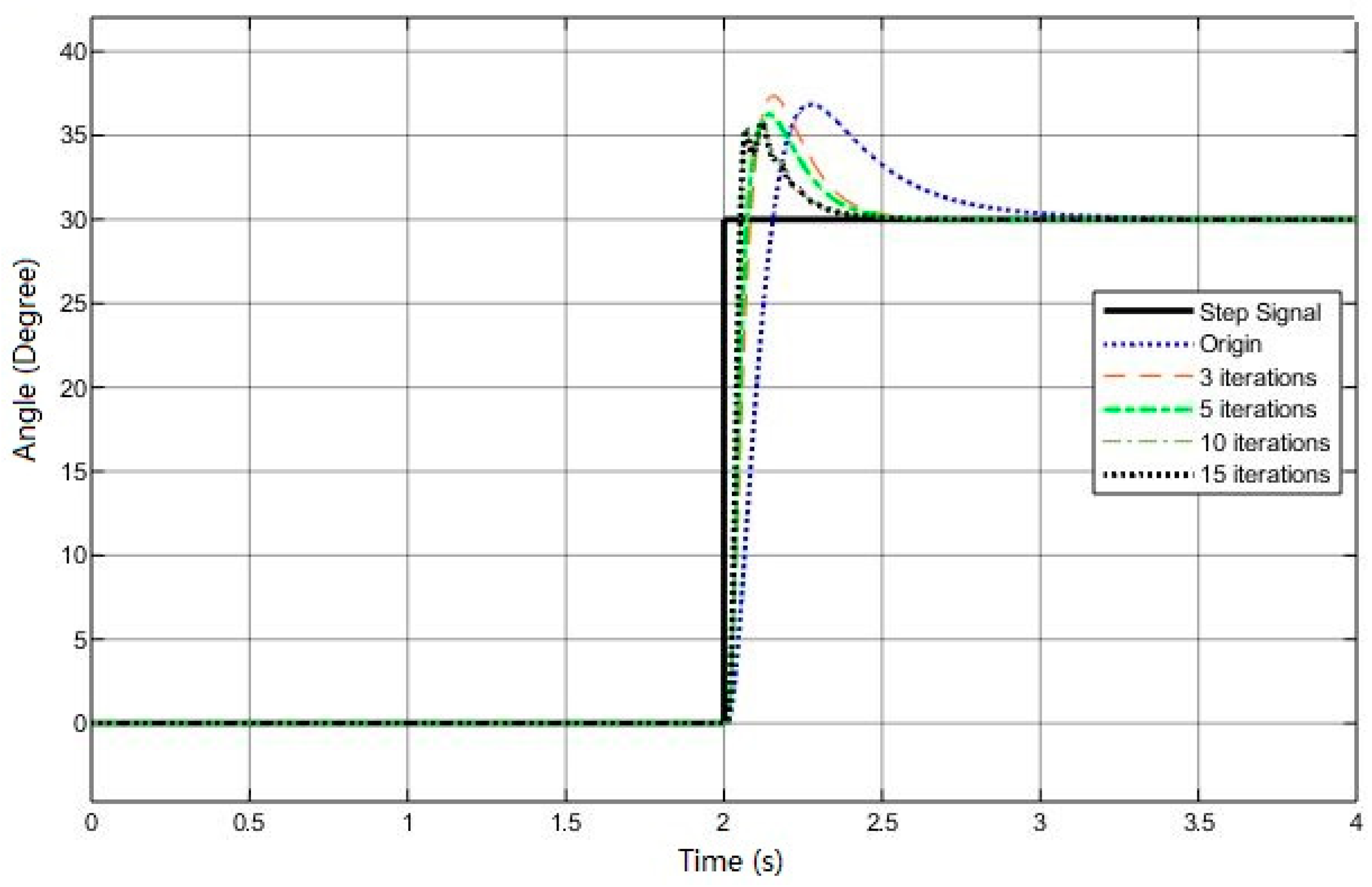
ITEA reflects the accumulated error in the control as an indicator to judge the performance of a controller. So, three coefficients refer to the position of a particle or a group of wolves. The smaller the ITAE, the better the position. Initially, the coefficients $m_1$, $n_1,$ and $n_2$ are 20, 4, and 4, respectively, these coefficients are based on some previous experiences and manual tunings. The step time of the input signal is at 2 s, and the final value is 30 degrees. The original ITAE is 8.616. The roll sub-controller has been optimised four times with the number of iterations 3, 5, 10, and 15 with the two optimisation approaches. With the increase in iterations, the ITAE reduced significantly. The detail of the comparisons is in

Table 1. PSO controller performance in term of ITAE.

PSO Iterations	m1	n1	n2	ITAE (rad s2)
0	20.0	4.00	4.00	8.616
3	17.96	7.34	22.71	6.056
5	19.66	13.26	24.59	5.540
10	35.77	11.04	36.91	4.153
15	37.91	10.61	38.03	4.097

for PSO and

Table 2. GWO controller performance in term of ITAE.

GWO Iterations	m1	n1	n2	ITAE (rad s2)
0	20.0	4.00	4.00	8.616
3	18.84	8.24	26.82	5.654
5	20.38	9.85	33.14	5.141
10	39.35	15.80	46.31	3.956
15	39.49	15.85	46.47	3.955

for GWO.

As can be seen from Table 1 and Table 2, the effectiveness of the two optimisation algorithms can be compared by comparing ITAE. GWO outperformed PSO by 6.6% and 7.2% in three and five iterations, respectively, in terms of optimisation; in 10 and 15 iterations, the advantage reduced to 4.7% and 3.5%. After more than ten iterations, the sub-controllers improved by both optimisation algorithms and were close to optimal. However, the performance of GWO is always slightly better than PSO. The coefficients were set to $w_1=2$and $w_2=2$. Other coefficients have been tried but with no better performance. The purpose of using these optimisation methods is to tune the controller. Still, the PSO itself also has coefficients that need to be adjusted. This includes its three coefficients and the initial direction of motion, which all impact the optimisation results. Whereas all the coefficients of the GWO are random numbers or can vary linearly depending on the number of iterations. The GWO shows better performance; therefore, the overall flight controller is optimised using GWO.

In

Table 3. Controller performance in terms of rise time, overshoot, and settling time.

GWO Iterations	Rise(s)	Peak (s)	Overshot (%)	Settle (s)
0	0.087	0.259	21.2	1.014
3	0.051	0.154	24.6	0.499
5	0.041	0.142	20.8	0.469
10	0.026	0.120	19.0	0.389
15	0.026	0.120	19.0	0.389

, the rise time, the peak time, the overshoot, and the settling time of each optimised roll sub-controller have been compared. All these four response parameters have improved after optimisation. The performances of the sub-controllers optimised over 10 and 15 iterations are very similar; there was only a 0.3% difference in the ITAE. The sub-controller with 15 iterations should be selected if only numerical results are considered. However, from Figure 5, in the performance of the sub-controllers with 10 and 15 iterations, when the simulated value exceeds the target value, there was some oscillation before reaching the peak. This oscillation occurs when the sub-controller has undergone more than five iterations of optimisation. When all rotation sub-controllers work in tandem, these oscillations can introduce further instability into the flight of the drone. So finally, the roll sub-controller, optimised through five iterations, was selected for further design. With the optimisation of five iterations, the rise time was reduced by 52.9%; the peak time was reduced by 45.2%, the overshot reduced by 1.9%, and the ITEA reduced by 59.7%. With the exception of the overshot, the improvement in all other aspects is remarkable.

The other sub-controllers have also been optimised by GWO with a similar process. The roll and pitch motions of the drone are very similar, so the pitch sub-controller used the same coefficients as the roll controller. These two sub-controllers were optimised first because they are essential for stable flight and are used to control the translational movement of the drone.

The yaw sub-controller has been optimised secondly. The control of the yaw angle is relatively less important than the other two attitude angles. Thus, when optimising the yaw sub-controller, it is also important to consider its influence on the other two attitude angles. The method used is to simultaneously give a 30 degrees step response command to all three attitude angles. To minimise the sum of the three angles ITAE is used as the optimisation target.

Then, the altitude sub-controller has been optimised. A 2 m step response was given to the system. The optimisation target is to minimise the ITAE of the motion in z-direction. The x and y sub-controllers have been optimised last as the thrust and attitude angles determine the translational motion. They need to be optimised based on the optimised rotation sub-controllers and the altitude sub-controller. The process is the same with the altitude sub-controller. Due to the similarity of the two translational movements, the two sub-controllers use the same coefficients. The original and optimal coefficients are shown in

Table 4. The original and optimised coefficients of other sub-controllers.

Coefficient	${\mathit{m}}_3$	${\mathit{n}}_5$	${\mathit{n}}_6$	${\mathit{m}}_4$	${\mathit{n}}_7$	${\mathit{n}}_8$	${\mathit{m}}_5\&{\mathit{m}}_6$	${\mathit{n}}_9\&{\mathit{n}}_{11}$	${\mathit{n}}_{10}\&{\mathit{n}}_{12}$
Original	1.60	0.90	3.20	5.00	10.00	3.00	2..50	1.00	1.00
Optimal	15.14	11.40	12.67	6.91	9.96	6.65	3.81	4.68	3.89
No. of Iterations	5			10			3

.

The optimisation effect of the roll angle sub-controller has been certified in a test bench. In addition, the entire flight controller has been verified in simulation with a designed trajectory.

5. Test Bench

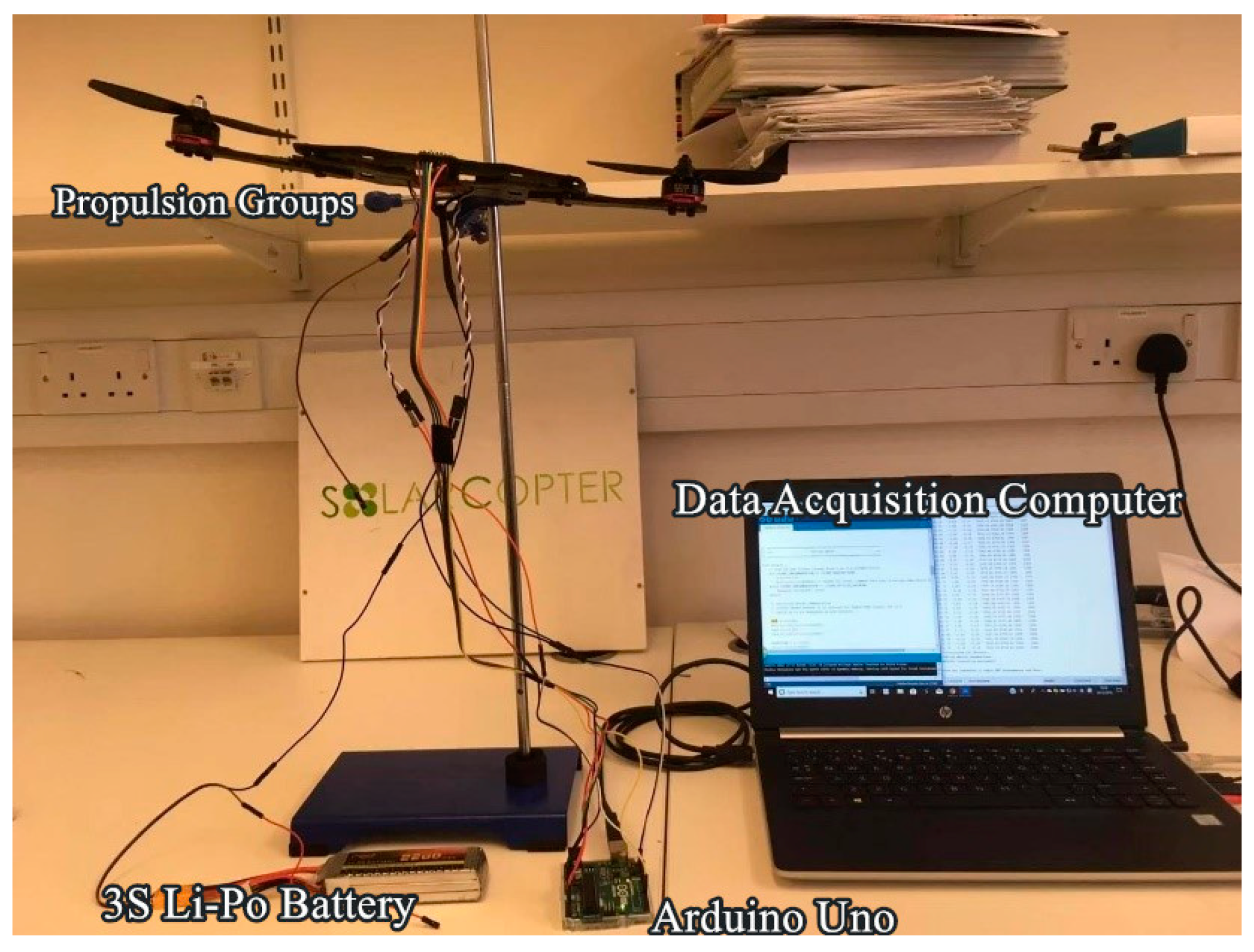
A preliminary test bench was carried out to test the flight controller. This test bench is a two-motor system, motors are fixed to the ends of a carbon fibre board, and an axis is fixed in the middle with a bearing, as shown in Figure 6. The system has one degree-of-freedom motion, the roll angle. The test bench helps lock some degrees of freedom to avoid system damage and reduce control complexity [6]. This test bench is equivalent to the roll motion of the drone; it was used to test the roll sub-controller. Using the following equation:

$$\begin{array}{c}{I}_{test}\ddot{{\theta }_t}=b{l}_t\left({\Omega }_1^2-{\Omega }_2^2\right)\end{array}$$

(44)

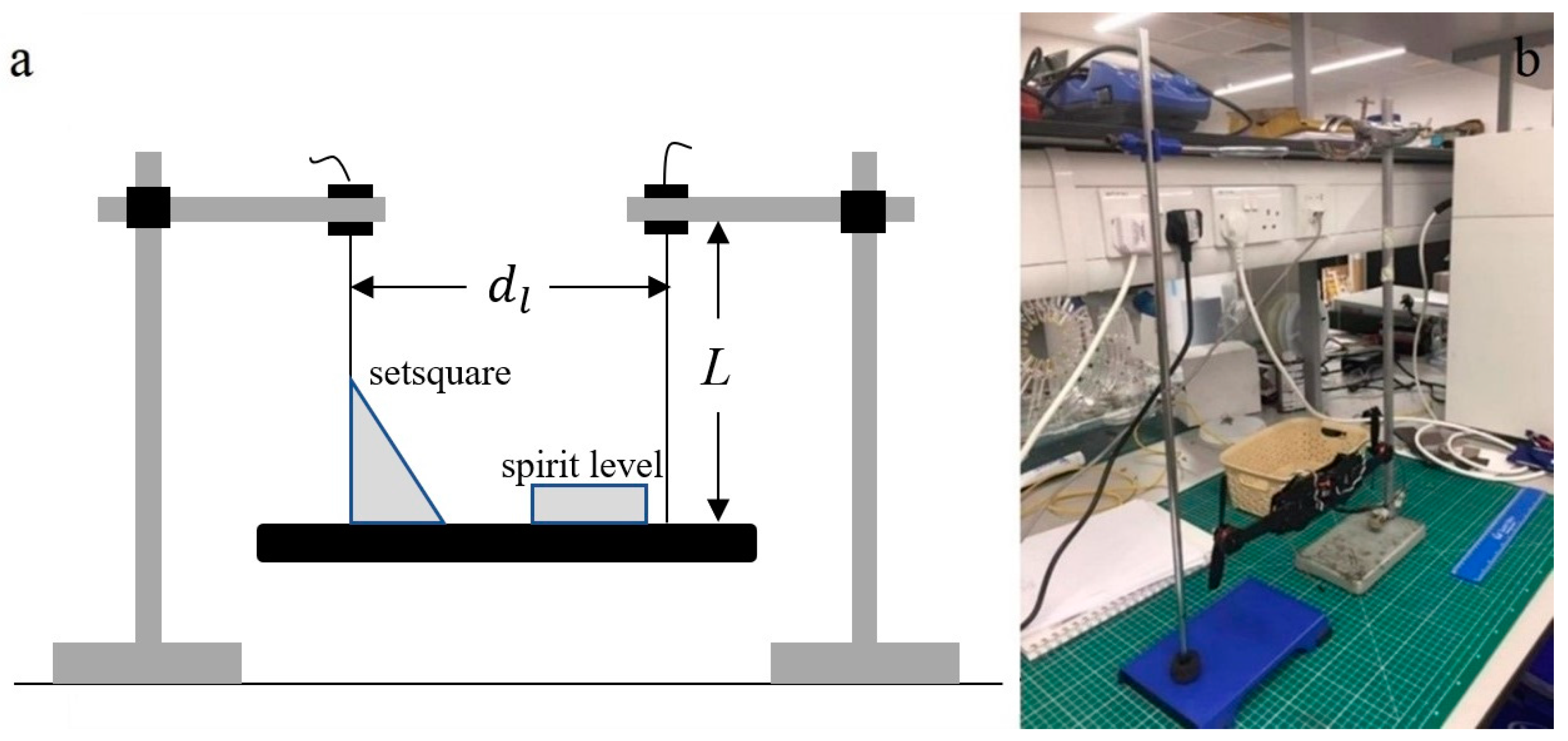
Where ${\theta }_t$ is the angle between the system and horizontal plane, it can be measured by an IMU, $l_t$ is the distance between propeller and axis, which is easy to measure, ${\Omega }_1$ and ${\Omega }_2$ are the speeds of the two propellers. $I_{test}$is the moment of inertia of this testing device. In this experiment, the moment of inertia of the system is measured by the oscillation of a bifilar suspension (Figure 7).

$$\begin{array}{c}{I}_{test}=\frac{m_{t}g{t}_b{}^2{d}_l{}^2}{16{\pi }^{2}L} \end{array}$$

(45)

The moment of inertia $I_{test}$ can be calculated using Equation (45). $m_t$is the mass of the system, $g$ is the acceleration due to gravity. $L$ is the rope length; $d_l$ is the distance between the wires; and $t_b$ is the period of the swing, which a stopwatch can measure. This test bench was applied to test the different controllers in the roll angle step response; the control algorithm was translated to codes and implemented to a microcontroller (Arduino Uno).

6. Results

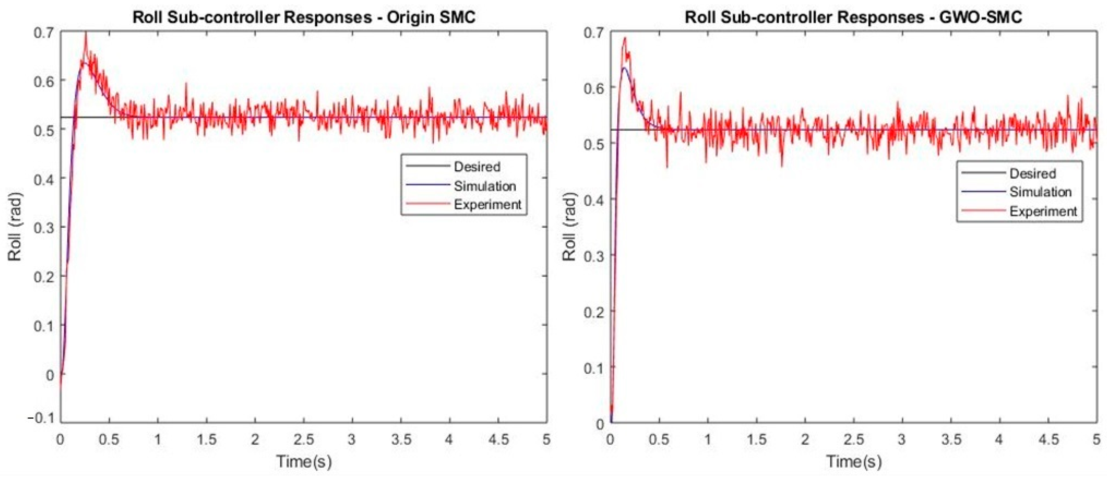
The optimised roll sub-controller was verified in the test bench, as shown in Figure 8 and

Table 5. Performance of the optimised roll sub-controller.

Indicator	IAE (rad s)	ITAE (rad s2)	E-IAE (rad s)	E-ITAE (rad s2)
Origin	0.069	0.012	0.155	0.231
GWO	0.042	0.005	0.125	0.207

. In quantitative analysis, the integration of absolute error (IAE, Equation (46)) is also used in the analysis. This indicator does not take time into account. IAE is more valuable in trajectory tracing. In Table 4, the IAE and ITAE in the simulation, as well as in the experiment are compared; E-ITAE and E-IAE refer to the ITAE and IAE in the experiment. In this step response, the step time is 0, so the ITAE is smaller than the simulation in the optimisation process. In the simulation, the IAE and ITAE were reduced by 39.13 and 58.33, respectively, while in the experiment, the E-IAE and E-ITAE were reduced by 19.35 and 10.39, respectively. The situation is caused by the vibration in the results given by the sensor, nevertheless, the effect of the optimisation is remarkable. Moreover, due to the results’ vibration, in Figure 8, it is difficult to visualise the difference between the original system and the optimised system.

$$\begin{array}{c} \mathrm{IAE}={{\displaystyle \int }}_0^{\infty }\left|e\left(t\right)\right|dt \end{array}$$

(46)

The whole optimised flight controller has been implemented in Simulink for simulation with the mathematical model. First, the inputs of the controller have to be confirmed. During the control of the autonomous flight, the system’s inputs are the desired position (x, y, z) and yaw angle ($\psi$). The outputs of the flight controller are the commanded speeds of the motors; the commanded speeds are inputted into the dynamical model for simulation.

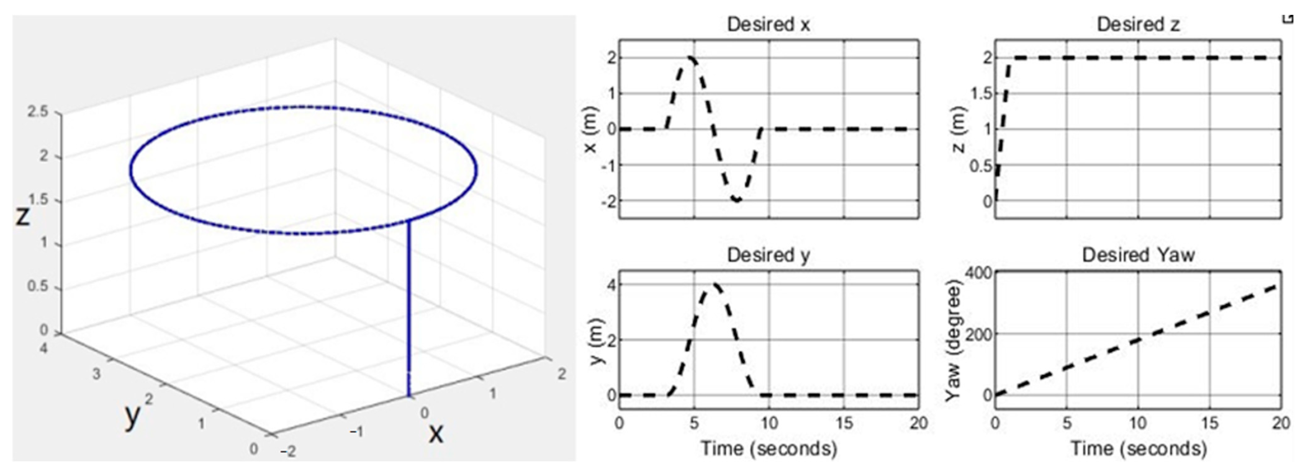
A trajectory was designed to test the flight controller to face extreme conditions. In the test trajectory, the drone rises 2 metres in the first second and then starts moving along a circular trajectory, and simultaneously the drone should rotate 360 degrees; the simulation time is 20 s. All the six degrees of freedom motion are involved in this trajectory. The equation of trajectory is as follows:

$$\begin{array}{c}\begin{array}{c}{x}_d\left(t\right)=x_{9d}\left(t\right)=\{\begin{array}{c} 0, 0\le t<\pi \\ -2sin\left(t\right), \pi \le t<3\pi \\ 0, t\ge 3\pi \end{array}\\ y_d\left(t\right)=x_{11d}\left(t\right)=\{\begin{array}{c} 0, 0\le t<\pi \\ 2\mathit{cos}\left(t\right)+2, \pi \le t<3\pi \\ 0, t\ge 3\pi \end{array}\\ z_d\left(t\right)=x_{7d}\left(t\right)=\{\begin{array}{c}2t, 0\le t<2\\ 2, t\ge 2\end{array}\\ {\mathsf{\psi }}_d\left(t\right)=x_{5d}\left(t\right)=\frac{\pi }{10}t\end{array}\end{array}$$

(47)

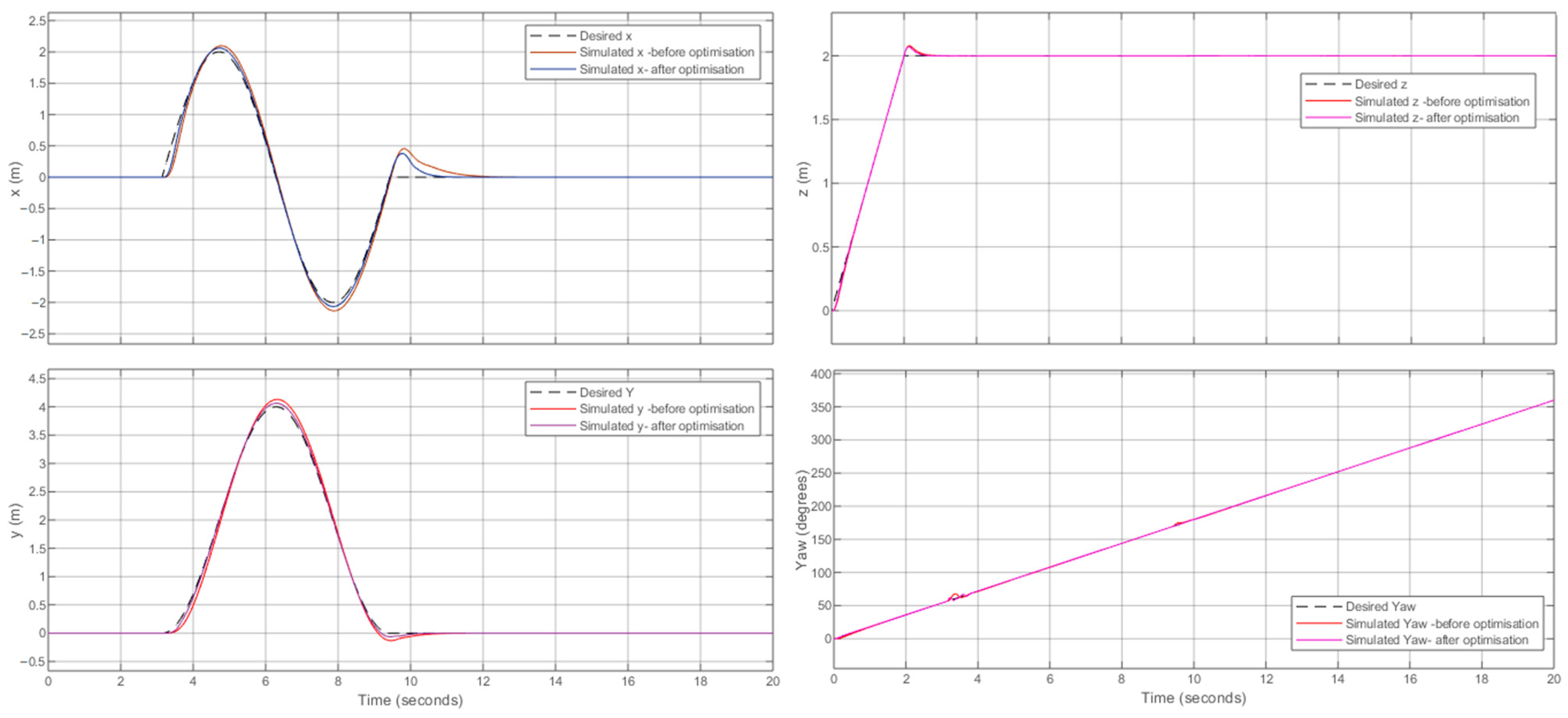
The trajectory is shown graphically in Figure 9. The designed trajectory was used to test both the original and optimised flight controller, and the results are presented in Figure 10 and Figure 11.

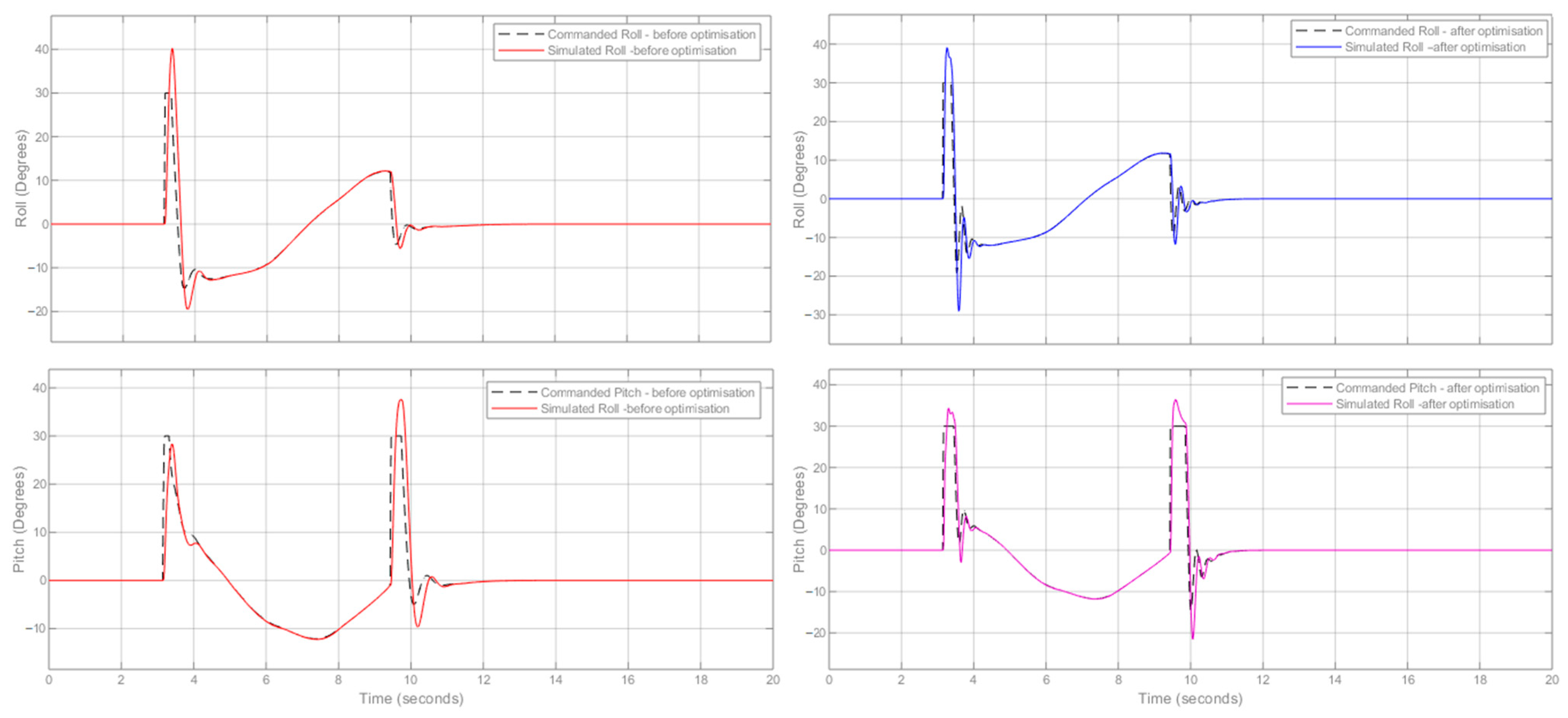
From 0 to 2 s, the drone started to rotate and rise; there was no translational movement or roll and pitch. From the $\pi$th second, the drone was required to move towards both x and y directions, so the commanded roll and pitch angle appeared. The commanded roll and pitch angle is limited to +/− 30 degrees in both original and optimised controllers to maintain a stable flight. The two figures clearly show that the drone with the optimised controller follows the designed trajectory more closely. This result does not only come from intuition but is confirmed numerically.

Quantitative analysis is more convincing. In

Table 6. Original and optimised comparison in IAE and ITAE.

	IAE-Roll (deg s)	ITAE-Roll (deg s2)	IAE-Pitch (deg s)	ITAE-Pitch (deg s2)	IAE-Yaw (deg s)	ITAE-Yaw (deg s2)
Origin	11.79	55.24	14.51	112.40	5.185	23.04
GWO	9.96	51.7	11.26	81.36	1.39	5.68
Improvement (%)	15.6	6.4	22.4	27.6	73.2	73.4
	IAE-x(ms)	ITAE-x(ms2)	IAE-y (ms)	ITAE-y (ms2)	IAE-z (ms)	ITAE-z (ms2)
Origin	1.15	8.73	0.80	4.53	0.06	0.09
GWO	0.60	4.37	0.29	1.92	0.04	0.06
Improvement (%)	47.8	50.0	63.8	57.6	33.3	33.3

, both ITAE and IAE in six degrees of freedom motion have been compared. ITAE is a kind of time-weighted measurement. Applying ITAE on step response is necessary, since it is important to consider a steady-state error. However, for this trajectory, some significant errors appear in the late stage due to the complexity of the desired value; it is not reasonable to compare ITAE in this case. So, the measurement without time weighted or IAE has been compared too. However, all the error measurements of the drone with optimised sub-controllers are smaller.

Table 6 also gives the percentage of the improvement. The most improved is the yaw sub-controller with 73.2% error reduction. The performance of the x and y sub-controllers has also improved by close to or more than 50%. Relatively small improvements were made to the altitude controller. Mainly the coefficients of the original z sub-controller are closer to optimal compared to the other sub-controllers. The above four sub-controllers, which receive direct commands regarding the desired trajectory, have all been significantly optimised. The roll and pitch controllers receive instructions from the position sub-controllers. When the position sub-controllers are optimised, the angle commands are given more aggressively to achieve a fast response. This poses a greater challenge to the roll and pitch sub-controllers. Despite this, the cumulative control error of the roll and pitch sub-controllers for the same trajectory is reduced by 15.6% and 22.4%. This is a further indication of the success of the optimisation.

7. Conclusions

The nonlinear dynamical model of a hexacopter drone has been simulated, and a flight controller based on sliding mode control theory has been developed and applied to the drone. The drone can fly autonomously following a desired trajectory. GWO was chosen to optimise the entire SMC flight controller on the basis of a comparative performance study of PSO and GWO on a sub-controller. The optimised sub-controller has improved in rise time, peak time, overshot, settle time, and ITAE. In theory, optimisation for a single angle sub-controller could result in a 58.3% reduction in ITAE. However, due to equipment limitations, only a 10.4% improvement was measured in the experiment. The entire flight controller has also been optimised. For the same trajectory tracking, the optimised controller shows a significant reduction in the IAE in each degree of freedom compared to the original controller. The optimisation is most evident in the yaw angle, where the cumulative error is reduced by 73.2%. In practice, these optimisations enable the drone to get to the desired location faster and more accurately and could make surveillance or information collection via cameras more accurate.