Dual-Anchor Metric Learning for Blind Image Quality Assessment of Screen Content Images

Abstract

The natural scene statistic is destroyed by the artificial portion in the screen content images (SCIs) and is also impractical for obtaining an accurate statistical model due to the variable composition of the artificial and natural parts in SCIs. To resolve this problem, this paper presents a dual-anchor metric learning (DAML) method that is inspired by metric learning to obtain discriminative statistical features and further identify complex distortions, as well as predict SCI image quality. First, two Gaussian mixed models with prior data are constructed as the target anchors of the statistical model from natural and artificial image databases, which can effectively enhance the metrical discrimination of the mapping relation between the feature representation and quality degradation by conditional probability analysis. Then, the distances of the high-order statistics are softly aggregated to conduct metric learning between the local features and clusters of each target statistical model. Through empirical analysis and experimental verification, only variance differences are used as quality-aware features to benefit the balance of complexity and effectiveness. Finally, the mapping model between the target distances and subjective quality can be obtained by support vector regression. To validate the performance of DAML, multiple experiments are carried out on three public databases: SIQAD, SCD, and SCID. Meanwhile, PLCC, SRCC, and the RMSE are then employed to compute the correlation between subjective and objective ratings, which can estimate the prediction of accuracy, monotonicity, and consistency, respectively. The PLCC and RMSE of the method achieved 0.9136 and 0.7993. The results confirm the good performance of the proposed method.

1. Introduction

The screen content image (SCI) is an important medium for human–computer interaction that can offer people a high standard of comfort and high-quality visual experiences. Thus, SCIs are extensively used in remote desktops, cloud computing, video games, multi-screen interaction, and other fields [1,2,3,4]. However, a great deal of noise will inevitably be involved in the process of image acquirement, transmission, and storage, which can lead to SCI image quality degradation and decrease people’s visual experience [5,6,7]. Thus, a reliable estimation of SCIs plays a critical role in the optimization of processing systems as guidance. Currently, image quality assessment (IQA) methods can be classified into three categories: full-reference (FR), reduced-reference (RR), and no-reference or blind (NR), based on the existence of reference image information. However, because the reference version of authentically distorted images is not available in most cases, constructing an effective blind image quality assessment (BIQA) method for SCIs has important research significance and practical application value.

1.1. Related Work

Many BIQA methods have progressed markedly in recent decades when analyzing natural images. However, these methods are not suitable for SCIs, as demonstrated in existing studies. The main reason is that the inherent characteristics of SCIs are quite different from those of natural images [8,9]. More specifically, SCIs are arbitrarily composed of natural and artificial parts via splicing or overlapping. The natural part is similar to natural images, containing rich and complex brightness and color distribution, but the artificial part is generally just the opposite. Therefore, the perception preferences exhibit a marked difference from the natural images. For this problem, some prior studies have been carried out in this field from different perspectives and can be roughly categorized into feature-inspired methods and neural network-based methods. The former methods, as the name implies, construct quality-aware features in the grayscale domain by fully considering the perceptual properties of SCIs for a certain aspect and then learning the mapping model between the obtained features and subjective quality to predict the distorted image quality. Gu et al. constructed 13 and 4 types of perceptual features to characterize image quality by analyzing the degradation mechanisms of structure, brightness, and so on [10,11]. Min et al. extracted and integrated the multiscale corner and edge features of SCIs [12]. Lu et al. extracted the orientation and structure features based on the orientation selectivity mechanism [13]. Fang et al. incorporated statistical brightness and texture features inspired by the human visual system [14]. Zheng et al. used the variance of the local standard deviation as a local feature and the hybrid region-based property as a global feature [15]. Fang et al. resorted to photometric invariant chromatic descriptors and local ternary pattern operators to measure the statistical features of the color and texture of SCIs, respectively [16]. Considering the redundancy of the spatial domain, some efforts have been devoted to representing these artificial feature vectors with more compact representations via sparse representation. Yang et al. characterized the local texture property of SCIs with the oriented gradient histogram and then represented these texture features using sparse coding [17]. Zhou et al. constructed the local and global dictionaries to achieve a fused quality representation for distorted SCIs [18]. Shao extracted quality-aware features by conducting local and global sparse representations for the corresponding regions [19]. Wu et al. leveraged sparse representation to extract the local structural feature and the global brightness feature [20]. Bai et al. learned content-specific codebooks to generate effective micro features [9] and further combined the macro features based on the Bernoulli law of large numbers for quality prediction [21]. In brief, these artificial features in the spatial or sparse domain can intuitively describe the content variations within each SCI, such as brightness, texture, and shape, and demonstrate moderate performance in legacy benchmark databases. However, limited by visual mechanisms and subjective knowledge, these features only focus on specific distortion types and cannot be authentically effective in revealing the essence of real-world distortions for SCIs.

Differing from feature-inspired methods, neural network-based methods make full use of end-to-end characteristics to capture the high-level features of SCIs, which can more efficiently characterize advanced semantic information by imitating human visual perception. Chen et al. designed a naturalization module composed of an upsampling layer and a convolutional layer for the quality prediction of SCIs [22]. Jiang et al. proposed a novel quadratic optimized model to optimize a deep convolutional neural network for SCIs [23]. Yue et al. designed a convolutional neural network for SCIs with the entire image instead of image patches as inputs [24]. Jiang et al. modified the convolutional neural network by treating image patches differently according to their contents [25]. Yang et al. proposed a multitask distortion-learning network by combining the distortion types and degree as prior knowledge to predict SCI quality [26]. Then, Yang et al. designed an AdaBoosting backpropagation neural network by integrating the contour and edge information with L-moment distribution estimation [27]. These high-level features are more adaptable to complex and specific tasks but lack intuition and interpretability due to the neural network’s characteristics. Moreover, because their performance often depends on the design of the network structure and the scale of the database, it is typically difficult to obtain an optimal model with good stability. Such models are also typically prone to underfitting or overfitting the results. In conclusion, current methods primarily focus on the feature extraction and neural network structure and do not attempt to describe the statistical characteristics of SCIs because the artificial part of SCIs destroys the natural scene statistics (NSS) features [28], which are widely used for BIQA of natural images and achieve very good effectiveness [29,30]. Bai et al. designed a lognormal pooling scheme to enhance the effectiveness of feature aggregation by analyzing the particularity of the statistical distribution of sparse codes [21]. Chen et al. introduced the correlation penalization between different feature dimensions, leading to features with lower ranks and higher diversity [31]. Yang et al. extracted the quality-aware features from the textual region and pictorial region [32]. Thus, finding a reliable statistical model which can be adopted to efficiently discriminate the intrinsic quality variations is still a marked challenge that must be overcome.

1.2. Contributions

To fill these gaps in knowledge, the dual-anchor metric learning (DAML) method is designed to evaluate the quality of distorted SCIs more accurately in this study. Considering that the NSS can easily be destroyed by the artificial portions of an SCI, it is difficult and impractical to obtain an accurate statistical model of SCIs. Inspired by metric learning, we do not deliberately seek an accurate statistical model of SCIs but rather construct a distance function to measure the similarity or difference degree with the available models and then apply the distance to identify the complex mixtures of distortions of SCIs. First, two available statistical models with prior data are constructed as the target anchors of the statistical model from two uncorrelated pristine databases. Then, the differences in the second-order statistics are softly aggregated between the local features and clusters of each target statistical model. Finally, the differences are used to predict the distorted image quality via support vector regression. Compared with other studies reported in the literature, the main contributions of this paper are summarized as follows:

• Metric learning is used to characterize the statistical features of SCIs, providing new thoughts and direction for the establishment of statistical feature models of complex scenes. Considering the variable composition of SCIs, statistical features cannot be accurately represented with a single statistical model but can be more reliably characterized by the measured distance with some available statistical models inspired by metric learning. In this paper, the dual-anchor and variance differences can contribute to the multi-aspect analysis of complex mixtures of SCI distortions, avoiding the dependence on some specific distortion types, and experimental results with three public SCI databases confirm the effectiveness of the proposed method.
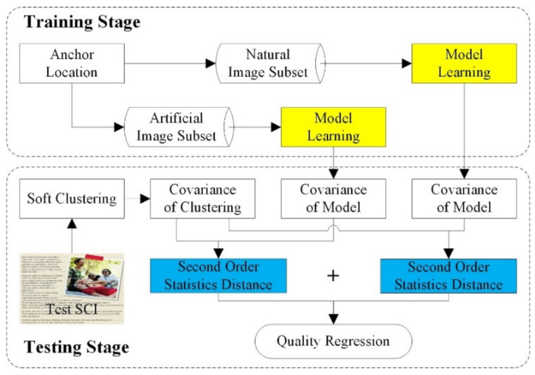
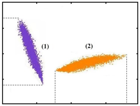
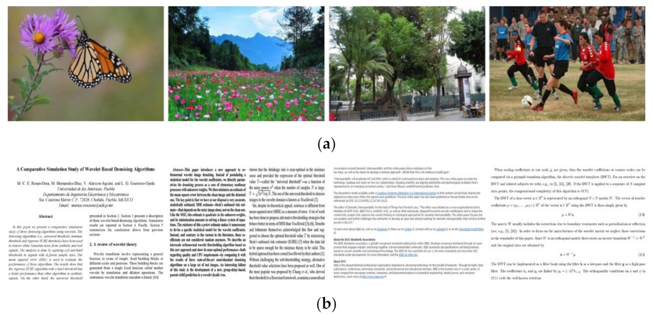
• The performance of metric learning is directly determined by the anchor point and metrics function. Most existing studies focused on generating a single statistical model with only one dataset, based on the assumption that each distortion follows a uniform distribution. However, this strategy fails to describe the statistical characteristics of SCIs due to the intricate content, variable composition, and composite mixtures of multiple distortions. Thus, we resort to a dual-anchor statistical model as the anchor point for SCIs in this study. First, two Gaussian mixed models (GMMs) with different characteristics are generated by representative datasets with unrelated images, and then both are used as the positive and negative anchor points. Specifically, the GMM is used as the statistical model of the anchor points for more informative scene representation, because the GMM is a linear combination of multiple Gaussian distribution functions and fully incorporates prior knowledge, which is theoretically suitable for the description of complex scene distributions. Meanwhile, the measured distances of high-order statistics are used as a metric function for efficient distance calculation, and only the variance differences are used as the quality-aware features in this study to balance complexity and effectiveness via empirical analysis and experimental verification.
• Both color and brightness information are combined via tensor decomposition to avoid information loss and optimize the structure of feature extraction. As mentioned above, existing methods primarily focus on feature generation in the grayscale domain and generally ignore color information. For tensor decomposition, the brightness and color information are fused perfectly in the principal component without missing the primary texture details. With that in mind, this component is employed as the carrier to train models and extract features in this paper, as well as acquire certain positive effects.

The remainder of this paper is organized as follows. In Section 2, the motivation and methodology of the proposed method are described in detail. Section 3 shows the experimental results and compares the performances with the state-of-the-art methods. Finally, Section 4 concludes the paper.

2. Materials and Methods

Considering that the artificial portion of SCIs destroys the NSS feature of natural scenes, we construct a dual-anchor metrics function to measure the high-order statistical differences with the existing statistical models inspired by metric learning and then apply them to identify the complex mixtures of distortions of SCIs. The flowchart of the proposed BIQA method is shown in Figure 1. Obviously, the proposed method involves two stages: offline model training and online quality prediction, which will elaborate the motivation and methodology of the anchor point and metrics function, respectively.

Specifically, the training stage involves anchor location and model learning, which are implemented offline with two collected pristine image datasets and will end once the two target GMMs have been trained. For the test SCI, only the testing stage is involved, and the quality prediction consists of two steps: feature generation and quality regression. Among them, feature generation softly aggregates the high-order statistical differences between the clusters of local features and the generated dual-anchor statistical models. Then, quality regression is performed via support vector regression (SVR) based on the combined statistical differences.

2.1. Offline Model Training

For metric learning, the distance function can be expressed as a set of points with the following relations: the sample points are similar or dissimilar anchors, and the metric function is optimal for distance calculation [33]. Thus, the performance of the distance function is directly determined by both the anchor point and metrics function. In this subsection, the influence of anchor points on the model reliability will be described in detail through two steps: anchor location and model learning.

2.1.1. Anchor Location

The core of metric learning is to predict the probability of subjective qualities for each image by calculating the similarity or difference between the learned statistical models. Thus, the models must be sensitive to the position in the feature space, and choosing an appropriate anchor can effectively improve the discrimination and expressiveness of the features, making it easier for the models to identify the degree of image distortion. For example, the statistical model of NSS features has been demonstrated to be stable and mature for natural images, and it has been mapped to predict the visual quality scores with efficient performance. However, for SCIs, artificial components, such as computer graphics and document contents, destroy these statistical features of natural scenes. To date, it is still impractical to obtain an accurate statistical model due to the variable composition of the artificial and natural parts in SCIs.

Assuming that two distortions of SCIs follow the distribution, as shown in Figure 2 with different colors and numbers, obviously, the metric accuracy of the distribution for each distortion is different when the distortion is projected on different axes. Taking the distribution of (1) in purple as an example, the performance of the statistical difference is markedly better when it is projected onto the vertical axis than when it is projected onto the horizontal axis. However, the opposite is true for the distribution of (2) in orange. These results indicate that using only a single anchor for the metric method is not sufficient to represent the specific characteristics of SCIs due to their intricate content, variable composition, and composite mixtures of multiple distortions. Thus, a more efficient method should be designed to convey authentically distorted image quality. As shown in Figure 2, a naive idea is to design some independent anchors and further employ the mutual constraints between these anchors to make the quality mapping of metric learning more robust. Obviously, the number of anchor points directly affects the robustness and complexity of the method. Thus, because SCIs are arbitrarily composed of artificial and natural portions, their image quality will be reduced with increasing noise intensity and types. The natural and artificial portions exhibit different statistical features from each other that are unrelated. Hence, two representative subsets, with the collected pristine natural images and artificial images shown in Figure 3, were built to characterize the extreme content characteristics of SCIs in two opposite directions and were then used to train the unrelated statistical models. Subsequently, both models were used as the positive and negative anchor points. The experimental results in Section 3 can verify the superiority of this dual-anchor statistical model.

The natural image dataset had a total of 90 images collected from TID [34] and LIVE [35] public datasets, and the artificial image dataset had a total of 100 document content images, where all pictures were obtained by manual screenshots. Considering the pristine natural image dataset as an example, the raw image was preprocessed first with tensor decomposition and other feature enhancement techniques, and then the constructed feature vector was used for subsequent model training. The specific process is described as follows.

First, tensor decomposition was employed to mitigate the fact that the color property had not been considered in the previous studies on BIQA of SCIs. As a form of higher-order principal component analysis, Tucker tensor decomposition can decompose a tensor $\chi \in {ℝ}^{I_1\times I_2\times \cdots I_N}$ into a core tensor $\varsigma \in {ℝ}^{J_1\times J_2\times \cdots J_N}$ multiplied (or transformed) by a group of matrices along each mode [36]. Specifically, a data cube of the RGB image can be converted into a three-order tensor as follows:

$$\chi \approx \varsigma {\times }_1{Y}^{\left(1\right)}{\times }_2{Y}^{\left(2\right)}{\times }_3{Y}^{\left(3\right)}$$

(1)

where $\chi \in R^{I_1\times }{{}^{I_2}}^{\times I_3}$; I₁, I₂, and I₃ are the sizes of the red, green, and blue channels of the raw image, respectively, and $Y^{\left(1\right)}$, $Y^{\left(2\right)}$, and $Y^{\left(3\right)}$ are the factor matrices with the same sizes of each channel, which are typically orthogonal. As mentioned in our previous study [21], we can draw the following conclusions. $Y^{\left(1\right)}$, as the principal component, basically preserves the texture details and brightness range. Meanwhile, the brightness property and color information are seamlessly combined. Thus, the principal component is adopted as the carrier of subsequent model training.

For the principal component, the raw patches, which are n × n in the grayscale domain, are all normalized with a divisive normalization transform to imitate the early nonlinear processing in the human visual system, reduce data redundancy, and maintain data consistency [37,38]:

$$\widehat{p}(i,j)=\frac{p(i,j)-\alpha }{\beta +\gamma }$$

(2)

where $p(i,j)$ and $\widehat{p}(i,j)$ are the raw and normalized patches of the principal component $Y^{\left(1\right)}$, respectively, (i, j) are the indices over the entire image, $\alpha$ and $\beta$ are the local mean and standard deviation of each patch, respectively, and $\gamma$ is a constant to prevent instability, which is set equal to 10 by the experience in this paper.

Aside from this, the whitening process is used in this paper to eliminate the linear correlations of each patch [39]. Finally, the global feature vector is constructed with these normalized image patches $\widehat{p}(i,j)$ to implement the subsequent model training.

2.1.2. Model Learning

After the anchor location mentioned above, how to construct two appropriate statistical models from two pristine databases, which are used as the target dual-anchor statistical models, must be determined. Selecting a model type is still a particular challenge for anchor points for each database.

As reported in the literature [40], Xu et al. presented a BIQA method for natural images based on high-order statistics aggregation (HOSA) with a small codebook, which calculated the differences of high-order statistics between the local features and corresponding clusters as the quality-aware image representation. In essence, this method is a simplified distance metric learning with a statistical model. Specifically, the codebook is equivalent to constructing a statistical model as an anchor point, and these statistics differences (i.e., mean, variance, and skewness) correspond to the distance measures of different orders. Each distortion pattern is characterized by a different kind of cluster, and this relative relationship varies with the distortion level. Therefore, the HOSA can measure the quality of the natural images more effectively.

However, the HOSA limit factors are more obvious for synthetic SCIs, one of which is the generality problem of the statistical model. For SCIs, the NSS feature of natural images is destroyed by the artificial portion, and no particularly reliable statistical model has been found to date due to the combined diversity of SCIs. If HOSA is directly transplanted to SCIs with only a single model (i.e., one anchor point), it does not exhibit effective performance compared with natural images, considering the varied and unpredictable distribution for the SCIs, as shown in Figure 2. Additionally, the statistical model of HOSA is constructed with a small codebook that contains only 100 codewords, which is relatively simple and suitable for natural scenes. However, the universality and robustness of this model seem to be marginally insufficient to reveal the statistical characteristics of SCIs due to the intricate content, variable composition, and composite mixtures of multiple distortions. Currently, the Gaussian mixed model (GMM) has been widely used to solve the situation where the data in the same set contain multiple different distributions, and it has achieved remarkable successes in many image processing tasks [41]. Compared with the limited codewords, the typical character is that the GMM is a linear combination of multiple Gaussian distribution functions which can theoretically fit any type of distribution by setting the cluster property. Therefore, the GMM was adopted as the target model to enhance the universality and robustness in this paper.

Meanwhile, HOSA lacks the effective guide provided by a priori information. For ill-conditioned problems, the core paradigm is to introduce a priori information to achieve the goal of discovering hidden and meaningful knowledge from limited data [42]. Hence, the a priori information must be applied reasonably to overcome shortages of limited feature information in the BIQA domain of SCIs and thus enhance the generalization and sensitivity of feature representation for SCIs. Two available GMMs with priors are constructed as the final statistical models in this paper, and the model learning process is illustrated as follows.

For the natural image dataset, we considered these normalized image patches $\widehat{p}(i,j)$ as local features and chose the VLFeat open-source library to implement GMM training [43]. For each image, N normalized patches are extracted such that $X=[{\widehat{p}}_1,{\widehat{p}}_2,\dots ,{\widehat{p}}_N]\in R^D(D=n\times n)$, where each column corresponds to one patch. Therefore, the constructed GMM for X can be described as $P_N(X\left|\rho ,\mu ,{\sigma }^2\right.)$, and

$$P_N(X)={\displaystyle {\sum }_{k=1}^K{\rho }_k\varphi (X\left|{\mu }_k,{\sigma }_k^2\right.)}$$

(3)

$$\varphi (X)=\frac{1}{\sqrt{2\pi }\sigma }\exp [-\frac{{(X-\mu )}^2}{2{\sigma }^2}]$$

(4)

where $P_N$ is the cumulative distribution function generated with the natural image dataset, $\rho$, $\mu$, and ${\sigma }^2$ are the prior, mean, and covariance of each feature in the GMM, respectively, ${\rho }_k\ge 0,{\displaystyle {\sum }_{k=1}^K{\rho }_k}=1$, and $\varphi (X)$ is the probability density function. In addition, K clusters of the GMM were constructed to capture various distortion characteristics. Similarly, the probability density function generated with the artificial image dataset is expressed as $P_A$. Note that this process is performed offline, and both GMMs ($P_N$ and $P_A$) can be applied directly as the target dual-anchor statistical model for feature learning of the test image without subsequent updates.

2.2. Online Quality Prediction

With the constructed GMMs ($P_N$ and $P_A$), the quality of testing SCIs could be predicted online with the following two steps: feature generation and quality regression. For feature generation, because the metric method will directly affect the accuracy of the quality prediction for each distortion beside the anchor points, the variance difference was selected as the target metric method through theoretical and empirical analysis in this study, considering the characteristics of the SCIs. Subsequently, SVR was performed to calculate the final quality score based on the combined statistical differences.

2.2.1. Feature Generation

In this subsection, we follow the line of HOSA to aggregate the statistical distances between the local features and clusters of the target dual-anchor statistical models (i.e., the two GMMs). Meanwhile, to tackle HOSA’s deficiency for SCIs, the a priori information of dual-anchor GMMs was extra extracted and used in feature generation, and only the second-order statistical differences were calculated as the quality-aware features to benefit the balance of complexity and effectiveness.

Here, the target dual-anchor statistical model consists of two GMMs ($P_N$ and $P_A$), and both GMMs are used in a similar process. For each single local feature ${\widehat{P}}_i$ of the test SCI, r nearest clusters rNN (xi) are selected by Euclidean distance. Soft assignment with kernel similarity weights attempts to alleviate the problems of uncertainty and plausibility in the clustering selection of the GMM without introducing large quantization error. In this paper, r is set to five based on the author’s experience.

Then, different order statistical distances were calculated with each prior as follows to further measure the degradation degree of the distorted image. The residual between the soft weighted mean, variance, skewness, and kurtosis of local features are assigned to cluster k and those of cluster k in the constructed GMM $P_N$ (or $P_A$):

$$M_k^d=\left({\widehat{\mu }}_k^d-{\mu }_k^d\right){\rho }_k^d=\left({\displaystyle {\sum }_{i:k\in rNN(x_i)}{\omega }_{ik}{x}_i^d}-{\mu }_k^d\right){\rho }_k^d$$

(5)

where ${\widehat{\mu }}_k^d$ and ${\mu }_k^d$ are the means of the dth dimension in cluster k for the local features and the target GMM $P_N$ (or $P_A$), respectively, ${\rho }_k^d$ is the prior of each feature in the GMM, the superscript d denotes the dth dimension of a vector, and ${\omega }_{ik}$ denotes the Gaussian kernel similarity weight between local feature xi and cluster k. The sum of the weights for each cluster is one. We also have

$$V_k^d=\left({\widehat{\sigma }}^2{}_k^d-{\sigma }^2{}_k^d\right){\rho }_k^d=\left[{\displaystyle \sum _{i:k\in rNN(x_i)}{\omega }_{ik}{(x_i^d-{\widehat{\mu }}_k^d)}^2}-{\sigma }^2{}_k^d\right]{\rho }_k^d$$

(6)

$$S_k^d=\left({\widehat{\gamma }}_k^d-{\gamma }_k^d\right){\rho }_k^d=\left\{{\displaystyle \sum _{i:k\in rNN(x_i)}[\frac{{\omega }_{ik}{(x_i^d-{\widehat{\mu }}_k^d)}^3}{{({\widehat{\sigma }}^2{}_k^d)}^{\frac{3}{2}}}]}-{\gamma }_k^d\right\}{\rho }_k^d$$

(7)

$$K_k^d=\left({\widehat{\kappa }}_k^d-{\kappa }_k^d\right){\rho }_k^d=\left\{{\displaystyle \sum _{i:k\in rNN(x_i)}[\frac{{\omega }_{ik}{(x_i^d-{\widehat{\mu }}_i^d)}^4}{{({\widehat{\sigma }}^2{}_k^d)}^2}]}-{\kappa }_k^d\right\}{\rho }_k^d$$

(8)

where ${({\widehat{\sigma }}^2)}_k^d$ and ${({\sigma }^2)}_k^d$ are the variances of the dth dimension in cluster k for the local features and the target GMM $P_N$ (or $P_A$), respectively. Similarly, ${\widehat{\gamma }}_k^d$ and ${\gamma }_k^d$ are the skewness of the dth dimension, and ${\widehat{\kappa }}_k^d$ and ${\kappa }_k^d$ are the kurtosis of the dth dimension.

Each statistical distance with different orders can characterize diverse image features. However, only the second-order statistical distances (i.e., variance differences) are employed to predict image quality in this study for the following reasons. For natural images, HOSA, which considers the mean, variance, and skewness, has demonstrated highly competitive performance with high-frequency information such as texture and details. Compared with natural images, SCIs generally have rich, complex artificial parts and fewer, simpler brightness or color variations and structures. In image processing, the variance, which can characterize the texture and edge properties of scenes, has been widely investigated and exhibits excellent comprehensive performance [40]. Considering that the image statistics aggregation method can describe the approximate location of an image’s local features in each cluster, and each distortion pattern is characterized by a different kind of cluster, the image quality will be more dramatically varied as the strength of the relative relationship increases. To avoid excessive complexity, it is intuitively obvious that the variance is an effective indicator of statistical characteristics for SCIs with larger artificial portions. The experimental results in the next section further validate the analysis compared with some combinations of different orders.

More specifically, we denote the second-order statistical difference with GMMs $P_N$ and $P_A$ as $v_k^N$ and $v_k^A$, respectively. Then, both second-order statistical differences are concatenated to a single long quality-aware feature: $f_k=[v_k^N{}^{\top },v_k^A{}^{\top }],k=1,2,\dots ,K$. Furthermore, there are some similar contents in SCIs and similar quality scores in subjective opinion scores, and these similarities increase image feature similarity, severely decrease the contribution of other important dimensions, and reduce overall feature effectiveness. Hence, elementwise signed power normalization was adopted on the aggregated features to alleviate the corruption caused by these similarities [44]. Specifically, each second-order local feature $\widehat{f}$ can be described as follows:

$$\widehat{f}=sign(f){\left|f\right|}^{\lambda }=[{\widehat{v}}^N{}^{\prime },{\widehat{v}}^A{}^{\prime }]$$

(9)

where $\lambda$ is the parameter to control the inhibition degree on the frequent components, which was set to 0.2 in this study. Finally, the entire quality-aware features, which are used for quality regression, can be denoted by

$$\widehat{F}=[{\widehat{f}}_1,{\widehat{f}}_2,\dots ,{\widehat{f}}_K]=[{\widehat{V}}^N,{\widehat{V}}^A]\in R^{D\times K\times 2}$$

(10)

where ${\widehat{V}}^N,{\widehat{V}}^A$ are the normalized second-order subfeatures with the GMMs $P_N$ and $P_A$, respectively.

2.2.2. Quality Regression

After feature generation, SVR was employed to learn a mapping function from normalized features to subjective quality scores for training SCIs [45]. Then, the quality score of the test SCI can be predicted with the pretrained regression model in the testing stage. Here, SVR with a radial basis function kernel was adopted by using the LIBSVM package with the default parameters [46].

In this study, the patch size D was set to 7 × 7, and the cluster number K was set to 100 based on the authors’ experience so that the quality-aware representation provided a vector of the dimensionality D × K = 4900 features (i.e., $\widehat{V}$) and D × K × 2 = 9800 (which is $\widehat{F}$) in total for each test SCI. The practical effect of each feature vector will be illuminated in detail in the next section.

2.3. Experimental Protocol

In this section, thorough experiments are conducted to demonstrate the effectiveness of the proposed method with three public SCI databases: the screen content image quality assessment database (SIQAD) [8], screen content database (SCD) [47], and screen content image database (SCID) [48]. A brief introduction of these datasets is shown in

Table 1. Brief introduction of three public SCI databases.

Database	Image Number		Distortion
	Reference	Distorted	Type	Level	Notes
SIQAD	20	980	7	7	Gaussian noise (GN), Gaussian blur (GB), motion blur (MB), contrast change (CC), JPEG, JPEG 2000 (J2K) and layer segmentation-based coding (LSC)
SCD	24	492	2	/	Screen content compression (SCC) and High-Efficiency Video Coding (HEVC)
SCID	40	1800	9	5	GN, GB, MB, CC, JPEG, J2K, color saturation change (CSC), SCC, and color quantization with dithering (CQD)

.

Specifically, in digital images, GN mainly originates from poor lighting or sensor noise during acquisition, GB is an image blur filter that uses a normal distribution to calculate the transformation of each pixel, MB is the apparent blurring of dragging traces caused by fast-moving objects, CC easily causes brightness and saturation distortion, J2K represents distortion caused by JPEG and JPEG2000 encoding, and HEVC also has distortion problems in encoding. The “type” and “level” in the table indicate the distortion category and distortion level, respectively.

Meanwhile, Pearson’s linear correlation coefficient (PLCC), Spearman’s rank order correlation coefficient (SRCC), and the root mean squared error (RMSE) are then employed to compute the correlation between the subjective and objective ratings, which can estimate the prediction of the accuracy, monotonicity, and consistency, respectively. Higher values for the SRCC and PLCC and a lower value for the RMSE are expected for an advanced quality prediction metric. In addition, a five-parameter nonlinear logistic function was employed to nonlinearly regress the quality ratings into a common range as follows [49]:

$$f(x)={\beta }_1[\frac{1}{2}-\frac{1}{1+e^{{\beta }_2(x-{\beta }_3)}}]+{\beta }_{4}x+{\beta }_5$$

(11)

where ${\beta }_i,i\in \{1,\dots ,5\}$ are the parameters to be fitted and x and $f(x)$ denote the raw predicted score and corresponding mapped scores, respectively.

Additionally, each database was randomly divided into training and testing subsets 1000 times, with 80% as the training dataset and the remainder as the testing dataset, and the median result was adopted as the final performance.

3. Results

3.1. Performance Comparison on the Overall Database

Here, we compare the proposed DAML with the following state-of-the-art FR-IQA and NR-IQA methods. Specifically, the FR methods include five classic methods built for natural images (PSNR, SSIM [50], FSIM [51], VSI [52] and VIF [53]) and five top methods built for SCIs (SVQI [54], SQE [55], EFGD [56], SRCNN [57], and QODCNN [23]). The NR methods include 10 feature-inspired methods (SIQE [11], OSM [13], NRLT [14], HRFF [15], PQSC [16], TFSR [17], LGFL [18], CLGF [20], CSC [9], and MTD [21]), and 5 neural network-based methods (PICNN [22], IGMCNN [24], SIQA-DF [25], MtDl [26], and ABPNN [27]). Note that the results were cited from the literature except with the classic methods for fairness, and “/” indicates that a value is not available in the following tables.

Table 2. Experimental results of the proposed and other FR-IQA methods on SIQAD, SCD, and SCID.

Method	SIQAD			SCD			SCID
	PLCC	SRCC	RMSE	PLCC	SRCC	RMSE	PLCC	SRCC	RMSE
PSNR	0.5869	0.5608	11.5859	0.861	0.8589	1.1273	0.7622	0.7512	9.1682
SSIM	0.5912	0.5836	11.5450	0.8696	0.8683	1.0953	0.7343	0.7146	9.6133
FSIM	0.5746	0.5652	11.6120	0.9019	0.9039	0.9585	0.7719	0.7550	9.0040
VSI	0.5403	0.5199	11.9380	0.8715	0.8719	1.0879	0.7550	0.7530	9.3470
VIF	0.8198	0.8065	8.1969	0.9028	0.9043	0.9542	0.8200	0.7969	8.1069
SVQI	0.8911	0.8836	6.4965	0.9158	0.9194	0.8909	0.8604	0.8386	7.2178
SQE	0.9040	0.8940	6.1150	0.9290	0.9310	0.8210	0.9150	0.9140	5.7610
EFGD	0.8993	0.8901	6.2595	/	/	/	0.8846	0.8774	6.6044
SR-CNN	0.9160	0.9080	5.6830	/	/	/	0.9390	0.9400	4.8300
QODCNN	0.9142	0.9066	5.8015	/	/	/	0.8820	0.8760	/
Proposed	0.9135	0.9023	5.8088	0.9316	0.9265	0.7993	0.8737	0.8576	6.8673

shows the experimental results of the FR methods on the SIQAD, SCD, and SCID, where the top three results in each case are highlighted in boldface. From this table, we can make the following observations. First, the classic FR methods for natural images could nnot be directly transferred to SCIs because they do not consider the peculiar perceptual properties of SCIs. Second, for the top FR-IQA methods for SCIs, their performance was markedly improved because the targeted features or network structures were constructed for some specific distortions in SCI databases, and the original reference could also provide more accurate and reliable feature information. However, the limiting factors were also strong for these methods, because it was difficult or not possible to obtain the reference in most cases. In contrast, we resorted to metric learning to extract the discriminative statistical features of SCIs and achieve comparable results with these top FR methods for SCIs.

Table 3. Experimental results of the proposed and other NR-IQA methods on SIQAD, SCD, and SCID.

Method	SIQAD			SCD			SCID
	PLCC	SRCC	RMSE	PLCC	SRCC	RMSE	PLCC	SRCC	RMSE
SIQE	0.7906	0.7625	8.7650	0.7168	0.7012	1.547	0.6343	0.6009	10.9483
OSM	0.8306	0.8007	7.9331	0.7068	0.6804	1.5301	/	/	/
NRLT	0.8442	0.8202	7.5957	0.9227	0.9156	0.8091	0.8377	0.8178	7.7265
HRFF	0.8520	0.8320	7.4150	/	/	/	/	/	/
PQSC	0.9164	0.9069	5.708	0.9362	0.9299	0.7746	0.9179	0.9147	5.4793
TFSR	0.8618	0.8354	7.4910	/	/	/	0.8017	0.7840	8.8041
LGFL	0.8280	0.7880	/	/	/	/	/	/	/
CLGF	0.8331	0.8107	7.9172	/	/	/	0.6978	0.6870	10.1439
CSC	0.9109	0.8976	5.8930	0.9182	0.9080	0.8721	0.8531	0.8377	7.3930
MTD	0.9162	0.9090	5.7111	0.9196	0.9123	0.8654	0.8811	0.8730	6.7031
PICNN	0.8960	0.8970	6.7900	/	/	/	0.8270	0.822	8.0130
IGMCNN	0.8834	0.8634	6.3971	/	/	/	0.8710	0.8663	6.4123
SIQA-DF	0.9000	0.8880	6.2422	/	/	/	0.8514	0.8507	7.0687
MtDl	0.9281	0.9214	5.611	/	/	/	0.9248	0.9233	5.4200
ABPNN	0.8529	0.8336	7.2817	/	/	/	0.7147	0.6920	10.3988
Proposed	0.9135	0.9023	5.8088	0.9316	0.9265	0.7993	0.8737	0.8576	6.8673

shows the experimental results of the NR methods on the SIQAD, SCD, and SCID, in which the results were primarily concentrated in the SIQAD and SCID in terms of test images and distortion types. From this table, we can see that most feature-inspired NR-IQA methods exhibited worse performance than that of the FR-IQA methods above, such as SIQE, OSM, NRLT, HRFF, TRSR, LGFL, and CLGF. In addition, the gap with the two excellent algorithms of PQSC and MTD was not obvious. The algorithm proposed in this paper was very close to the data of the CSC and MTD in the SIQAD and SCID databases, respectively, and the indicators in the SCD database were even better. The main reason for this is that, limited by the research progress of visual perception and the attention preference of designers, these manual features show excessive subjectivity and independence from each other, which makes it difficult to accurately characterize and measure the intrinsic quality variations of SCIs if there is a lack of reference information. Due to the diversity of the SCI content, it was necessary to explore a more unified and complete theoretical system to reduce the loss of important information and serious subjective preferences for partial distortion types. For neural network-based methods, such as SIQA-DF and MtDl, they showed comparable performance to these FR methods because these high-level features are more adaptable to complex and specific tasks but lack intuition and interpretability, and this can easily lead to overfitting due to the neural network characteristics. In addition, Table 3 shows that the proposed method can effectively describe the distribution characteristics of the SCIs by constructing a distance function to measure the similarity or difference degree with two available uncorrelated statistical models. Finally, the proposed method achieved excellent performance in the PLCC compared with the feature-inspired methods and obtained competitive performance that was comparable to that of the neural network-based methods.

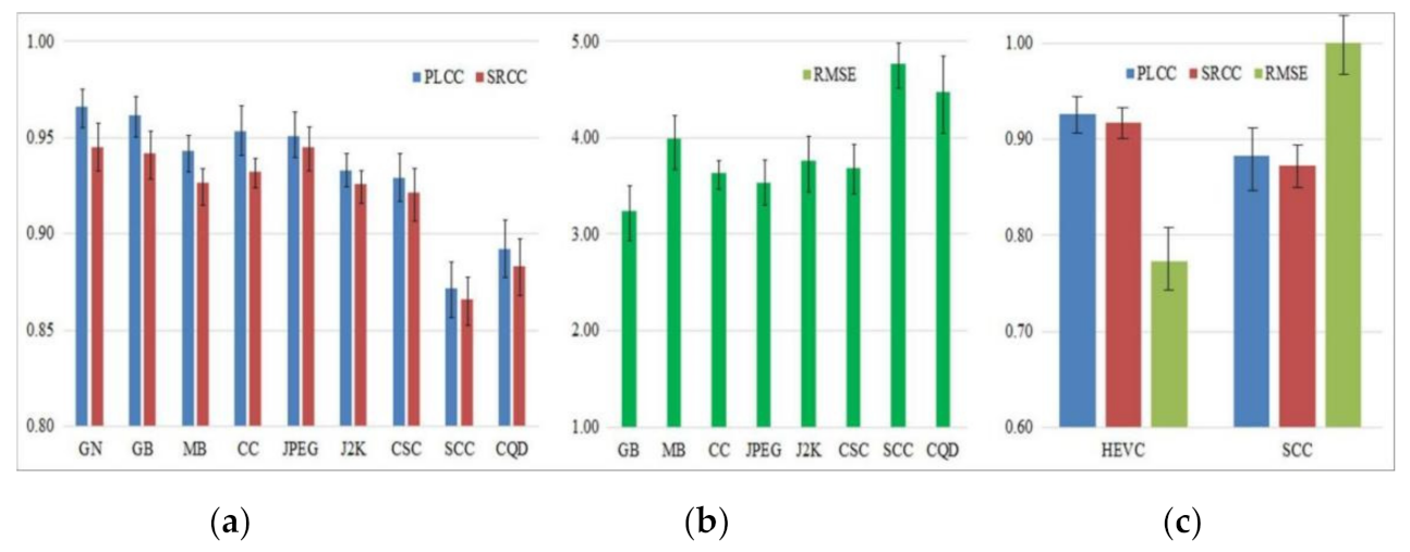
3.2. Performance Comparison of the Individual Distortion Type

To verify the performance of the individual distortion type, we investigated the model performances with the proposed DAML and other state-of-the-art methods on three SCI databases. Specifically,

Table 4. PLCC results of different distortion types for the proposed and other methods on SIQAD.

PLCC	GN	GB	MB	CC	JPEG	J2K	LSC	Variance
SIQE	0.8779	0.9138	0.7836	0.6856	0.7244	0.7339	0.7332	7.30 × 10−3
OSM	/	/	/	/	/	/	/
NRLT	0.9131	0.8949	0.8993	0.8131	0.7932	0.6848	0.7228	8.17 × 10−3
HRFF	0.9020	0.8900	0.8740	0.8260	0.7630	0.7540	0.7700	4.08 × 10−3
PQSC	0.9200	0.9300	0.9100	0.8200	0.8500	0.8900	0.8500	1.75 × 10−3
TFSR	0.9291	0.9367	0.9243	0.6563	0.8334	0.8347	0.8069	9.84 × 10−3
LGFL	0.9030	0.9110	0.8370	0.6600	0.7620	0.6680	0.6830	1.20 × 10−2
CLGF	0.8577	0.9082	0.8609	0.7440	0.6598	0.7463	0.5575	1.55 × 10−2
CSC	0.9317	0.9148	0.8846	0.9229	0.9036	0.9143	0.9294	2.67 × 10−4
MTD	0.9390	0.9156	0.8844	0.9231	0.914	0.8949	0.9192	3.28 × 10−4
PICNN	0.9100	0.9190	0.8890	0.8260	0.8290	0.8520	0.8360	1.56 × 10−3
IGMCNN	/	/	/	/	/	/	/	/
SIQA-DF	0.9120	0.9240	0.8900	0.8440	0.8290	0.8280	0.8580	1.56 × 10−3
MtDl	/	/	/	/	/	/	/	/
ABPNN	0.9139	0.9225	0.8948	0.7772	0.8014	0.7984	0.7907	4.14 × 10−3
Proposed	0.9400	0.9131	0.8946	0.9219	0.9176	0.9119	0.9328	2.21 × 10−4

,

Table 5. SRCC results of different distortion types for the proposed and other methods on SIQAD.

SRCC	GN	GB	MB	CC	JPEG	J2K	LSC	Variance
SIQE	0.8517	0.9174	0.8347	0.6874	0.7438	0.7241	0.7337	7.00 × 10−3
OSM	/	/	/	/	/	/	/	/
NRLT	0.8966	0.8812	0.8919	0.7072	0.7698	0.6761	0.6978	9.80 × 10−3
HRFF	0.8720	0.8630	0.8500	0.687	0.7180	0.7440	0.7400	5.94 × 10−3
PQSC	0.9000	0.9200	0.8900	0.7	0.8300	0.8800	0.8300	5.53 × 10−3
TFSR	0.9144	0.9311	0.9148	0.6498	0.8377	0.8354	0.7948	9.61 × 10−3
LGFL	0.8790	0.8940	0.8320	0.487	0.7440	0.6450	0.6660	2.16 × 10−2
CLGF	0.8478	0.9152	0.8694	0.5716	0.6778	0.7681	0.5842	1.93 × 10−2
CSC	0.9143	0.8971	0.8708	0.9075	0.8848	0.8911	0.9064	2.27 × 10−4
MTD	0.9201	0.8993	0.8703	0.9102	0.8966	0.8593	0.8867	4.61 × 10−4
PICNN	0.9020	0.9160	0.8800	0.6990	0.8230	0.8340	0.8720	5.36 × 10−3
IGMCNN	/	/	/	/	/	/	/	/
SIQA-DF	0.9010	0.9100	0.8800	0.7280	0.8120	0.8160	0.8580	4.06 × 10−3
MtDl	/	/	/	/	/	/	/	/
ABPNN	0.9102	0.9223	0.8867	0.7471	0.7768	0.7783	0.7585	5.92 × 10−3
Proposed	0.9212	0.8944	0.8834	0.9102	0.8993	0.8851	0.9061	1.87 × 10−4

and

Table 6. RMSE results of different distortion types for the proposed and other methods on SIQAD.

RMSE	GN	GB	MB	CC	JPEG	J2K	LSC	Variance
SIQE	8.1416	6.4239	8.0783	9.1565	6.4778	7.6727	6.3160	1.1861
OSM	/	/	/	/	/	/	/	/
NRLT	6.3113	6.9171	6.4524	7.8433	5.872	6.5441	5.7864	0.4858
HRFF	6.2670	6.7380	6.4660	6.8740	5.8620	6.5010	5.4730	0.2442
PQSC	/	/	/	/	/	/	/
TFSR	5.3105	5.2141	5.5266	10.5005	5.2541	5.6377	5.6217	3.7067
LGFL	/	/	/	/	/	/	/	/
CLGF	/	/	/	/	/	/	/	/
CSC	5.3292	5.3767	6.0794	5.0375	5.5912	5.4480	5.2539	0.1074
MTD	5.0506	5.2992	6.1017	5.0238	5.3266	5.9826	5.5994	0.1837
PICNN	6.2010	5.8700	5.7720	7.0120	5.4700	5.9920	4.6730	0.5049
IGMCNN	/	/	/	/	/	/	/	/
SIQA-DF	6.1150	5.7680	5.7910	6.7470	5.3840	5.8120	4.4620	0.4870
MtDl	/	/	/	/	/	/	/	/
ABPNN	5.9745	5.7319	6.7144	8.0684	6.8006	6.5538	5.4556	0.7584
Proposed	4.9987	5.3785	5.8043	4.9994	5.1861	5.4307	5.1030	0.0841

show the experimental results of PLCC, SRCC, and the RMSE, respectively, and the top three metrics are highlighted in boldface. Note that the variances were calculated to describe the fluctuation magnitude for each distortion type, and a lower value indicates better prediction consistencies. From these tables, it is obvious that most existing methods showed obvious preferences for specific distortion types, particularly for TFSR, LGFL, and CLGF. For example, CLGF handled the GB distortion with a PLCC of 0.9082, but its PLCC was only 0.5575 for the LSC distortion. Similarly, LGFL handled the GB distortion with an SRCC of 0.8940, but its SRCC was only 0.4870 for the CC distortion. The primary reason for this result is that these quality-aware features, which are extracted by existing methods, are subjective, independent, and limited by visual mechanisms and subjective knowledge. Thus, they merely reflect the quality degradation characteristics of some parts and cannot authentically and effectively describe the essence of real-world distortions for SCIs. In contrast, the proposed method combines metric learning and probability distribution to construct the discriminative statistics feature, identify complex distortions, and predict SCI image quality from a global perspective. Thus, the proposed method exhibited better generalization performance across different distortion types, producing variances that were orders of magnitude lower than those of other methods, as shown in Table 4, Table 5 and Table 6. In particular, it can be clearly seen that the proposed model was more sensitive to handling most distortion types (i.e., GN, CC, JPEG, J2K, and LSC) and exhibited good competitiveness with other types (i.e., GB and MB).

Additionally, Figure 4 presents similar results on the SCD and SCID for different distortion types. Thus, these results suggest that the proposed MADL can more precisely and steadily describe various degenerations from the perspective of statistical characteristics and distributions for SCIs and can further verify the effectiveness and robustness of the proposed method. The data and results are shown in Table 4, Table 5 and Table 6, where SIQAD was a commonly used data set and we listed the detailed evaluation data. SCD is the dataset that mainly tests coding distortion, so the data given are relatively small, while for SCID, the dataset is relatively large. The “/” in the table indicates that the article did not test it in detail, and there was no relevant code to reproduce and calculate the relevant indicators.

3.3. Cross-Database Validation

In this subsection, cross-database validation is conducted to verify the generalizability of the proposed DAML. Because SIQAD and SCID were the representative and largest databases, respectively, and both of them contained six distortion types (GN, GB, MB, CC, JPEG, and J2K), both databases were adopted as the training and testing databases, respectively. Similar to the practice of Mittal et al. [39] and Ye et al. [58], the DAML was trained on one database with these six distortion types, and the other was used to test the performance of the trained model. Meanwhile, the median performance is reported in this paper. Note that entire samples of both databases were adopted for model training and testing, which could reduce dependence on the scale of the database and further verify the generalizability of the proposed method [21].

Table 7. Cross validation results of the proposed DAML with six types of distortion on SIQAD and SCID.

Distortion	(a) Training with SIQAD			(b) Training with SCID
	PLCC	SRCC	RMSE	PLCC	SRCC	RMSE
GN	0.9300	0.9109	4.6213	0.8921	0.8843	6.7399
GB	0.9277	0.9088	4.4339	0.8551	0.8544	6.9978
MB	0.9059	0.8886	5.1253	0.8232	0.8317	7.6019
CC	0.8794	0.8605	5.8277	0.8236	0.8377	7.5378
JPEG	0.8359	0.8226	6.3599	0.8405	0.8365	7.2293
J2K	0.7148	0.6977	7.4051	0.7631	0.7546	7.2196
Overall	0.8541	0.8583	6.1862	0.8395	0.8438	7.4497

shows the cross-database results for each type of distortion, in which (a) means that the model was trained with SIQAD and tested with SCID, and (b) means the opposite. From this table, we can obtain the following observations. First, both cross-database performances were similar to each other, which indicates that the proposed model had the advantages of high generalization ability, regardless of database size and complexity. Second, the cross-database performance was marginally worse than the in-database performance, which is also a common problem for existing methods. The primary reason for this result is that different fusion rules that are caused by variable image compositions and distortion intensities of the SCI can generate complex degradation mechanisms and statistical properties for each SCI database and further result in performance degradation for each method. Third, the cross-database performance decreased for the proposed model but still achieved satisfactory performance and stability for most distortion types, achieving competitive performance compared with the FR methods in Table 2 and outstanding performance compared with most of the feature-inspired NR methods in Table 3. Note that the performance on the J2K type was lower than those of other distortion types because it belonged to the complex composite compression distortion.

In addition, the proposed cross-database performance was marginally worse than the neural network-based methods listed in Table 3 but was still worthy of affirmation considering its interpretability. Thus, the cross-database results demonstrate that the proposed method achieved good prediction accuracy, powerful stability, and generalization.

3.4. Ablation Study

To further verify the effectiveness of the proposed DAML, comparative experiments were conducted on three SCI databases. More specifically, these factors primarily include the anchor type, K value, and feature type. Among them, the anchor type and K value are defined based on the anchor location and model learning during offline model training, respectively, and the feature type is defined during feature generation of online quality prediction. In this study, the sensitivity of each factor is discussed with different settings, and then comparative experiments are performed to validate the influence of the parameter setting.

For metric learning, the type and number of anchor points are the most important factors to be considered first. Because the deficiency of a single anchor point was illustrated in detail in Section 2.1, it will not be repeated in this study, and the two anchors were set as the defaults in this study. Considering the anchor type, a naive idea is that two unrelated image types are used as the positive and negative anchor points to characterize some extreme content characteristics of SCIs in two opposite directions. Intuitively, there are two appropriate anchor types in terms of distortion intensity and content composition for SCIs. For distortion intensity, the reference images and distortion images can be adopted as the targeted anchors, which can directly describe the condition of quality distortion. For content composition, natural images and document images are suitable choices to directly describe the characteristics of the content composition in SCIs.

Table 8. Prediction performance with different anchor types.

Anchor Type	SIQAD			SCD			SCID
	PLCC	SRCC	RMSE	PLCC	SRCC	RMSE	PLCC	SRCC	RMSE
Reference + Distortion	0.9023	0.8901	6.1512	0.9287	0.9223	0.8193	0.8647	0.8503	7.1126
Natural + Artificial	0.9135	0.9023	5.8088	0.9316	0.9265	0.7993	0.8737	0.8576	6.8673

shows the comparison of the prediction performances with different anchor types. Performances were markedly improved with both anchor types, which effectively clarified the feasibility of the dual-anchor strategy. Meanwhile, the performance of the content composition was marginally better than that of the distortion intensity. The primary reason for this result is that distortion intensities exist for both natural images and SCIs, but the most distinctive aspect of SCIs lies in the arbitrary composition and random combination of different contents compared with natural images.

With the anchor type of the content composition, model learning has become another bottleneck of performance improvement for metric learning. Considering the characteristics of the content composition, the GMM was adopted as the target model in this study because it could solve the situation containing multiple different distributions in the same set. However, for the GMM, the value of K, which denotes the number of clusters, directly influenced the trade-off of performance and complexity. In this study,

Table 9. Prediction performance with different values of K.

K	SIQAD			SCD			SCID
	PLCC	SRCC	RMSE	PLCC	SRCC	RMSE	PLCC	SRCC	RMSE
50	0.9108	0.8979	5.8894	0.9282	0.922	0.8186	0.8657	0.8496	7.0651
100	0.9135	0.9023	5.8088	0.9316	0.9265	0.7993	0.8737	0.8576	6.8673
150	0.9103	0.8995	5.9006	0.934	0.9309	0.7868	0.8733	0.8572	6.8921

shows the comparison of the prediction performances with different values of K. Obviously, there were only marginally different performances for each K value, and thus we set K equal to 100 as the default according to the actual results in Table 9.

For online quality prediction, the selection of the feature type is a critical step for feature generation and directly affects the efficiency of quality regression. In this study, we constructed the experiments with different feature type combinations on three SCI databases and compared the results with HOSA on the SIQAD, which are shown in

Table 10. Experimental results of prediction performance with different feature types.

Feature Type	SIQAD			SCD			SCID
	PLCC	SRCC	RMSE	PLCC	SRCC	RMSE	PLCC	SRCC	RMSE
Mean	0.8961	0.8814	6.3428	0.9262	0.9220	0.8309	0.8586	0.8419	7.2503
Variance	0.9135	0.9023	5.8088	0.9316	0.9265	0.7993	0.8737	0.8576	6.8673
Skewness	0.8901	0.8774	6.5002	0.9048	0.9012	0.9385	0.8368	0.8189	7.7403
Kurtosis	0.8689	0.8529	7.0789	0.9227	0.9168	0.8544	0.7943	0.7746	8.5951
M. + V.	0.8978	0.8864	6.2922	0.9241	0.9209	0.8429	0.8526	0.8384	7.3896
M. + V. + S.	0.8783	0.8657	6.8292	0.9040	0.9111	0.9396	0.8175	0.8046	8.1537
M. + V. + S. + K.	0.8774	0.8655	6.8522	0.9030	0.9116	0.9485	0.8150	0.7995	8.1756

and

Table 11. Comparison of prediction performances with HOSA on SIQAD.

Feature Type	HOSA			Proposed
	PLCC	SRCC	RMSE	PLCC	SRCC	RMSE
Mean	/	0.8137	/	0.8961	0.8814	6.3428
Variance	/	0.8340	/	0.9135	0.9023	5.8088
Skewness	/	0.8159	/	0.8901	0.8774	6.5002
M. + V.	/	0.8343	/	0.8978	0.8864	6.2922
M. + V. + S.	0.8636	0.8484	6.9594	0.8783	0.8657	6.8292

, respectively. Note that the feature types used in this study include the first-order (mean), second-order (variance), third-order (skewness), and fourth-order (kurtosis) statistics, as well as the combinations of each other. In the two tables, “M.”, “V.”, “S.”, and “K.” denote the abbreviations for the mean, variance, skewness, and kurtosis statistics, respectively. Table 11 shows that all feature types had certain effects on image degradation, but the sensitivity of each type was different. Particularly after the optimization of the dual-anchor strategy, the performance of a single feature type (i.e., variance) was better than that of the feature combination, which could effectively enhance the efficiency of quality regression. Meanwhile, compared with HOSA built for natural images, the proposed method achieved better improvement on the SIQAD due to some of the following reasons: (1) the dual-anchor strategy makes quality mapping of metric learning more robust for varied content and the distortion of SCIs; (2) the GMM model can theoretically fit any type of distribution, which is particularly suitable for solving the situation of containing multiple different distributions in SCIs; and (3) the introduction of a priori information can further discover hidden and meaning knowledge from limited data.

4. Conclusions

This paper presented a dual-anchor metric learning method for blind image quality assessment for screen content images (SCIs). Inspired by metric learning, the statistical distance between the local features and clusters of the target dual-anchor model were resorted to represent the statistics feature and then predict the distorted image quality of SCIs. The target dual-anchor statistical model consisted of two Gaussian mixed models generated from unrelated pristine databases to avoid dependence on specific distortion types. The high-order statistical differences were further optimized and enhanced the effectiveness of quality-aware feature extraction. On three public SCI databases, the experimental results verified the superior prediction accuracy and generalizability of the proposed method for individual distortion types compared with the state-of-the-art blind image quality assessment methods of SCIs.

References

1. Kuang, W.; Chan, Y.; Tsang, S.; Siu, W. Machine learning-based fast intra mode decision for HEVC screen content coding via decision trees. IEEE Trans. Circuits Syst. Video Technol. 2020, 30, 1481–1496. [Google Scholar] [CrossRef]
2. Strutz, T.; Möller, P. Screen content compression based on enhanced soft context formation. IEEE Trans. Multimed. 2020, 22, 1126–1138. [Google Scholar] [CrossRef]
3. Tsang, S.; Chan, Y.; Kuang, W. Mode skipping for HEVC screen content coding via random forest. IEEE Trans. Multimed. 2019, 21, 2433–2446. [Google Scholar] [CrossRef]
4. Chen, J.; Ou, J.; Zeng, H.; Cai, C. A fast algorithm based on gray level co-occurrence matrix and Gabor feature for HEVC screen content coding. J. Vis. Commun. Image Represent. 2021, 78, 103–128. [Google Scholar] [CrossRef]
5. Cheng, S.; Zeng, H.; Chen, J.; Hou, J.; Zhu, J.; Ma, K. Screen content video quality assessment: Subjective and objective study. IEEE Trans. Image Process. 2020, 29, 8636–8651. [Google Scholar] [CrossRef]
6. Zhang, L.; Li, M.; Zhang, H. Fast intra bit rate transcoding for HEVC screen content coding. IET Image Process. 2018, 12, 738–744. [Google Scholar] [CrossRef]
7. Kuang, W.; Chan, Y.; Tsang, S.; Siu, W. Online-learning-based Bayesian decision rule for fast intra mode and cu partitioning algorithm in HEVC screen content coding. IEEE Trans. Image Process. 2020, 29, 170–185. [Google Scholar] [CrossRef]
8. Yang, H.; Fang, Y.; Lin, W. Perceptual quality assessment of screen content images. IEEE Trans. Image Process. 2015, 24, 4408–4421. [Google Scholar] [CrossRef]
9. Bai, Y.; Yu, M.; Jiang, Q.; Jiang, G.; Zhu, Z. Learning content-specific codebooks for blind quality assessment of screen content images. Signal Process. 2019, 161, 248–258. [Google Scholar] [CrossRef]
10. Gu, K.; Zhai, G.; Lin, W.; Yang, X.; Zhang, W. Learning a blind quality evaluation engine of screen content images. Neurocomputing 2016, 196, 140–149. [Google Scholar] [CrossRef]
11. Gu, K.; Zhou, J.; Qiao, J.; Zhai, G. No-reference quality assessment of screen content pictures. IEEE Trans. Image Process. 2017, 26, 4005–4018. [Google Scholar] [CrossRef]
12. Min, X.; Ma, K.; Gu, K.; Zhai, G.; Wang, Z.; Lin, W. Unified blind quality assessment of compressed natural, graphic, and screen content images. IEEE Trans. Image Process. 2017, 26, 5462–5474. [Google Scholar] [CrossRef] [PubMed]
13. Lu, N.; Li, G. Blind quality assessment for screen content images by orientation selectivity mechanism. Signal Process. 2018, 145, 225–232. [Google Scholar] [CrossRef]
14. Fang, Y.; Yan, J.; Li, L.; Wu, J.; Lin, W. No reference quality assessment for screen content images with both local and global feature representation. IEEE Trans. Image Process. 2018, 27, 1600–1610. [Google Scholar] [CrossRef]
15. Zheng, L.; Shen, L.; Chen, J.; An, P.; Luo, J. No reference quality assessment for screen content images based on hybrid region features fusion. IEEE Trans. Multimed. 2019, 21, 2057–2070. [Google Scholar] [CrossRef]
16. Fang, Y.; Du, R.; Zuo, Y.; Wen, W.; Li, L. Perceptual quality assessment for screen content images by spatial continuity. IEEE Trans. Circuits Syst. Video Technol. 2020, 30, 4050–4063. [Google Scholar] [CrossRef]
17. Yang, J.; Liu, J.; Jiang, B.; Lu, W. No reference quality evaluation for screen content images considering texture feature based on sparse representation. Signal Process. 2018, 153, 336–347. [Google Scholar] [CrossRef]
18. Zhou, W.; Yu, L.; Zhou, Y.; Qiu, W.; Wu, M.; Luo, T. Local and global feature learning for blind quality evaluation of screen content and natural scene images. IEEE Trans. Image Process. 2018, 27, 2086–2095. [Google Scholar] [CrossRef]
19. Shao, F.; Gao, Y.; Li, F.; Jiang, G. Toward a blind quality predictor for screen content images. IEEE Trans. Syst. Man Cybern. Syst. 2018, 48, 1521–1530. [Google Scholar] [CrossRef]
20. Wu, J.; Xia, Z.; Zhang, H.; Li, H. Blind quality assessment for screen content images by combining local and global features. Digit. Signal Process. 2019, 91, 31–40. [Google Scholar] [CrossRef]
21. Bai, Y.; Zhu, Z.; Jiang, G.; Sun, H. Blind quality assessment of screen content images via macro-micro modeling of tensor domain dictionary. IEEE Trans. Multimed. 2020, 23, 4259–4271. [Google Scholar] [CrossRef]
22. Chen, J.; Shen, L.; Zheng, L.; Jiang, X. Naturalization module in neural networks for screen content image quality assessment. IEEE Signal Process. Lett. 2018, 25, 1685–1689. [Google Scholar] [CrossRef]
23. Jiang, X.; Shen, L.; Feng, G.; Yu, L.; An, P. An optimized CNN-based quality assessment model for screen content image. Signal Process. Image Commun. 2021, 94, 116181. [Google Scholar] [CrossRef]
24. Yue, G.; Hou, C.; Yan, W.; Choi, L.; Zhou, T.; Hou, Y. Blind quality assessment for screen content images via convolutional neural network. Digit. Signal Process. 2019, 91, 21–30. [Google Scholar] [CrossRef]
25. Jiang, X.; Shen, L.; Ding, Q.; Zheng, L.; An, P. Screen content image quality assessment based on convolutional neural networks. J. Vis. Commun. Image Represent. 2020, 67, 102–745. [Google Scholar] [CrossRef]
26. Yang, J.; Bian, Z.; Zhao, Y.; Lu, W.; Gao, X. Staged-learning: Assessing the quality of screen content images from distortion information. IEEE Signal Process. Lett. 2021, 28, 1480–1484. [Google Scholar] [CrossRef]
27. Yang, J.; Bian, Z.; Liu, J.; Jiang, B.; Lu, W.; Gao, X.; Song, H. No-reference quality assessment for screen content images using visual edge model and adaboosting neural network. IEEE Trans. Image Process. 2021, 30, 6801–6814. [Google Scholar] [CrossRef]
28. Gu, K.; Wang, S.; Yang, H.; Lin, W.; Zhai, G.; Yang, X.; Zhang, W. Saliency-guided quality assessment of screen content images. IEEE Trans. Multimed. 2016, 18, 1098–1110. [Google Scholar] [CrossRef]
29. Saad, M.A.; Bovik, A.C.; Charrier, C. Blind image quality assessment: A natural scene statistics approach in the DCT domain. IEEE Trans. Image Process. 2012, 21, 3339–3352. [Google Scholar] [CrossRef]
30. Jiang, Q.; Shao, F.; Jiang, G.; Yu, M.; Peng, Z. Supervised dictionary learning for blind image quality assessment using quality-constraint sparse coding. J. Visual Commun. Image Represent. 2015, 33, 123–133. [Google Scholar] [CrossRef]
31. Chen, B.; Li, H.; Fan, H.; Wang, S. No-Reference Screen Content Image Quality Assessment with Unsupervised Domain Adaptation. IEEE Trans. Image Process. 2021, 30, 5463–5476. [Google Scholar] [CrossRef] [PubMed]
32. Yang, J.; Zhao, Y.; Liu, J.; Jiang, B.; Meng, Q.; Lu, W.; Gao, X. No Reference Quality Assessment for Screen Content Images Using Stacked Autoencoders in Pictorial and Textual Regions. IEEE Trans. Cybern. 2022, 52, 2798–2810. [Google Scholar] [CrossRef] [PubMed]
33. Kulis, B. Metric learning: A survey. Found. Trends Mach. Learn. 2012, 5, 287–364. [Google Scholar] [CrossRef]
34. Ponomarenko, N.; Ieremeiev, O.; Lukin, V.; Egiazarian, K.; Jin, L.; Astola, J.; Vozel, B.; Chehdi, K.; Carli, M.; Battisti, F.; et al. Color Image Database TID2013: Peculiarities and Preliminary Results. In Proceedings of the Europian Workshop on Visual Information Process. EUVIP, Paris, France, 10–12 June 2013; IEEE: Piscataway, NJ, USA, 2013; pp. 106–111. [Google Scholar]
35. Kang, L.; Ye, P.; Li, Y.; Doermann, D. Convolutional Neural Networks for No-Reference Image Quality Assessment. In Proceedings of the IEEE Conference on Computer Vision and Pattern Recognition, Columbus, OH, USA, 23–28 June 2014; IEEE: Piscataway, NJ, USA, 2014; pp. 1733–1740. [Google Scholar]
36. Kolda, T.G.; Bader, B.W. Tensor decompositions and applications. SIAM Review. 2009, 51, 455–500. [Google Scholar] [CrossRef]
37. Lyu, S.; Simoncelli, E.P. Nonlinear image representation using divisive normalization. In Proceedings of the 2008 IEEE Conference on Computer Vision and Pattern Recognition (CVPR), Anchorage, AK, USA, 23–28 June 2008; IEEE: Piscataway, NJ, USA, 2014; pp. 1–8. [Google Scholar]
38. Mittal, A.; Moorthy, A.K.; Bovik, A.C. No-reference image quality assessment in the spatial domain. IEEE Trans. Image Process. 2012, 21, 4695–4708. [Google Scholar] [CrossRef]
39. Hyvärinen, A.; Oja, E. Independent component analysis: Algorithms and applications. Neural Netw. 2000, 13, 411–430. [Google Scholar] [CrossRef]
40. Xu, J.; Ye, P.; Li, Q.; Du, H.; Liu, Y.; Doermann, D. Blind Image Quality Assessment Based on High Order Statistics Aggregation. IEEE Trans. Image Process. 2016, 25, 4444–4457. [Google Scholar] [CrossRef]
41. Lin, H.; Chuang, J.; Liu, T. Regularized background adaptation: A novel learning rate control scheme for Gaussian mixture modeling. IEEE Trans. Image Process. 2011, 20, 822–836. [Google Scholar]
42. Akkaynak, D.; Treibitz, T. A revised underwater image formation model. In Proceedings of the 2018 IEEE/CVF Conference on Computer Vision and Pattern Recognition (CVPR), Salt Lake City, UT, USA, 18–23 June 2018; IEEE: Piscataway, NJ, USA, 2018; pp. 6723–6732. [Google Scholar]
43. VLFeat Open Source Library. Available online: http://www.vlfeat.org/ (accessed on 8 August 2022).
44. Perronnin, F.; Sánchez, J.; Mensink, T. Improving the Fisher kernel for large-scale image classification. In Proceedings of the European Conference on Computer Vision (ECCV), Crete, Greece, 5–11 September 2010; pp. 143–156. [Google Scholar]
45. Chang, C.; Lin, C. LIBSVM: A library for support vector machines. ACM Trans. Intell. Syst. Technol. 2011, 2, 1–27. [Google Scholar] [CrossRef]
46. Zhou, C.; Yu, W.; Huang, K.; Zhu, H.; Li, Y.; Yang, C.; Sun, B. A New Model Transfer Strategy Among Spectrometers Based on SVR Parameter Calibrating. IEEE Trans. Instrum. Meas. 2021, 70, 1–13. [Google Scholar] [CrossRef]
47. Wang, S.; Gu, K.; Zhang, X.; Lin, W.; Zhang, L.; Ma, S.; Gao, W. Subjective and objective quality assessment of compressed screen content images. IEEE J. Emerg. Sel. Topics Circuits Syst. 2016, 6, 532–543. [Google Scholar] [CrossRef]
48. Ni, Z.; Ma, L.; Zeng, H.; Lin, W.; Zhang, L.; Ma, S.; Gao, W. SCID: A database for screen content images quality assessment. In Proceedings of the 2017 International Symposium on Intelligent Signal Processing and Communication Systems (ISPACS), Xiamen, China, 6–9 November 2017; IEEE: Piscataway, NJ, USA, 2017; pp. 774–779. [Google Scholar]
49. Gottschalk, P.G.; Dunn, J.R. The five-parameter logistic: A characterization and comparison with the four-parameter logistic. Anal. Biochem. 2005, 343, 54–65. [Google Scholar] [CrossRef] [PubMed]
50. Wang, Z.; Bovik, A.; Sheikh, H.; Simoncelli, E. Image quality assessment: From error visibility to structural similarity. IEEE Trans. Image Process. 2004, 13, 600–612. [Google Scholar] [CrossRef] [PubMed]
51. Zhang, L.; Zhang, L.; Mou, X.; Zhang, D. FSIM: A feature similarity index for image quality assessment. IEEE Trans. Image Process.. 2011, 20, 2378–2386. [Google Scholar] [CrossRef]
52. Zhang, L.; Shen, Y.; Li, H. VSI: A visual saliency-induced index for perceptual image quality assessment. IEEE Trans. Image Process. 2014, 23, 4270–4281. [Google Scholar] [CrossRef]
53. Sheikh, H.R.; Bovik, A.C. Image information and visual quality. IEEE Trans. Image Process. 2006, 15, 430–444. [Google Scholar] [CrossRef]
54. Gu, K.; Qiao, J.; Min, X.; Yue, G.; Lin, W.; Thalmann, D. Evaluating quality of screen content images via structural variation analysis. IEEE Trans. Vis. Comput. Graph. 2018, 24, 2689–2701. [Google Scholar] [CrossRef]
55. Zhang, Y.; Chandler, D.M.; Mou, X. Quality assessment of screen content images via convolutional neural network-based synthetic/natural segmentation. IEEE Trans. Image Process. 2018, 27, 5113–5128. [Google Scholar]
56. Wang, R.; Yang, H.; Pan, Z.; Huang, B.; Hou, G. Screen content image quality assessment with edge features in gradient domain. IEEE Access. 2019, 7, 5285–5295. [Google Scholar] [CrossRef]
57. Chen, C.; Zhao, H.; Yang, H.; Peng, C.; Yu, T. Full reference screen content image quality assessment by fusing multi-level structure similarity. ACM Trans. Multimed. Comput. Commun. Appl. 2020, 17, 1–21. [Google Scholar]
58. Ye, P.; Kumar, J.; Doermann, D. Beyond human opinion scores: Blind image quality assessment based on synthetic scores. In Proceedings of the IEEE Conference on Computer Vision and Pattern Recognition (CVPR), Columbus, OH, USA, 23–28 June 2014; IEEE: Piscataway, NJ, USA, 2014; pp. 4241–4248. [Google Scholar]
Figure 1. Flowchart of the proposed DAML method for SCIs.
Electronics 11 02510 g001
Figure 2. Simplified distortion diagram of different distributions for SCIs.
Electronics 11 02510 g002
Figure 3. Some examples of the collected pristine images for model learning: (a) natural images and (b) artificial images.
Electronics 11 02510 g003
Figure 4. Experimental results of different distortion types for the proposed method. (a) PLCC and SRCC values on SCID. (b) RMSE values on SCID. (c) PLCC, SRCC, and RMSE values on SCD.
Electronics 11 02510 g004