Distributed Radar Target Detection Based on RF-SSA in Non-Gaussian Noise

Abstract

Distributed radar target detection in non-Gaussian noise, modeled as the sum of K-distributed clutter plus thermal noise, is considered in this paper. The conventional target techniques, e.g., constant false-alarm rate (CFAR), scatterer density-dependent generalized likelihood ratio test (SDD-GLRT), and energy integration (EI) detectors, have limited performance. On the other hand, since radar target detection can be considered a classification task, deep learning techniques have been widely applied as radar detectors in recent years, but such techniques require a larger amount of training samples to prevent overfitting, which is time-consuming. To balance detection efficiency and accuracy, this paper proposes an improved random forest algorithm based on the sparrow search algorithm (RF-SSA). First, we propose a mixed method of 3DT space-time adaptive processing and wavelet denoising (3DT-WD) to improve the output signal-to-clutter plus-noise ratio. Then, the SSA is applied to the RF algorithm to adaptively obtain the optimal parameters of the detection model. The simulation results show that the proposed RF-SSA ensures higher detection performance than the other classical methods, showing a gain of about 2 dB at the same detection probability. Moreover, the detection results of the real data further confirm the superiority of the proposed RF-SSA.

1. Introduction

A target can be resolved into several discrete physical scatterers that appear in radar range cells for a high-resolution radar (HRR), which is regarded as a distributed target. Returned signals for HRR convey abundant target information, and they fluctuate less than that of low-range resolution radars. Therefore, HRRs can significantly enhance the target detection performance [1,2]. However, the detection strategies of the point-target may fail in practical high-resolution radar systems [3].

Distributed target detection has been extensively investigated in recent years, such as the adaptive detection of distributed targets in homogeneous environments [4]. In [5], the time-frequency distribution features of two adjacent echoes are utilized for target detection. By adding a general window function to calculate the cross S-method (CSM), it can efficiently detect targets with a high velocity, even if the adjacent radar high-resolution range profiles (HRRPs) are weakly correlated. By compensating for linear and quadratic phase errors [6], a waveform contrast-based constant false-alarm rate (CFAR) detector is proposed to realize the distributed radar target detection [7]. In [8], a persymmetric adaptive matched filter (perAMF) detector is proposed for the distributed target detection in Gaussian clutter, where the clutter covariance matrix is unknown. Numerical examples show that the perAMF detector still has good detection performance even though the training data is limited. In [9], by exploiting a priori knowledge of the clutter covariance matrix, an effective detection algorithm is proposed.

However, the assumption of the Gaussian random variable (RV) may no longer be met for the background clutter in HRRs. More specifically, the clutter can be described as non-Gaussian observations, which are suitable to be modeled by a spherically invariant random vector (SIRV) [10,11]. Recently, the adaptive detection of distributed targets in non-Gaussian clutter has been an active research topic in the radar community. For instance, in [12], based on the assumption of knowing the disturbance covariance matrix, an approximate generalized likelihood ratio test (GLRT) -based detector is designed. Similarly, a modified adaptive detector based on GLRT is devised in [13]. However, a priori knowledge about the disturbance covariance matrix in some complex electromagnetic environments is in general unknown. A detection method based on the volume cross-correlation function is proposed to solve this problem, without resorting to a priori knowledge about the disturbance covariance matrix [14]. However, its performance can be obtained by resorting to the basis vectors of the signal subspace, which is computationally burdensome.

The detection performance of distributed targets in non-Gaussian clutter depends not only on the detection algorithms but also on the performance of clutter compression. For instance, the space-time adaptive processing (STAP) technique plays a significant role in suppressing the sea/ground clutter by the co-development of degrees-of-freedom (DOFs) in both spatial and temporal domains. However, the performance of the traditional STAP technique may greatly degrade in heterogeneous clutter environments. To address this problem, several detection methods based on the estimation of the clutter covariance matrix (CCM) are devised [15,16]. However, the detection performances of the aforementioned methods significantly degraded when prior assumptions on clutter echoes deviate from the real clutter environments. To solve the problem, a robust detection method for STAP applications based on the volume cross-correlation function (VCF) is proposed and it does not need to estimate the clutter CCM. However, when the velocities of moving targets are unknown, or all the targets have different velocities, this method needs to slide the window with an unknown length along all the range axis to select the training sample matrix, which results in a huge computational burden [17].

In essence, target detection can be considered a binary classification task, and detection based on machine learning techniques has drawn much attention in recent several years. Amongst those techniques, deep learning techniques are being used as radar detectors with success [18]. For instance, in [19], the long short-term memory (LSTM) algorithm is used to achieve target detection with remarkable precision, even for very low SCR ratios. In [20], a dual neural network detection scheme is proposed, in which the first neural net is used to filter out noisy images, and the second neural net is used to realize target detection and classification by extracting fast-time and slow-time information. In [21], to lower the false alarm rate while maintaining the detection probability, an artificial neural network is proposed after applying a CFAR algorithm. However, those methods require a larger amount of training samples. Moreover, in general, a great increment in the number of samples leads to an increase in the training time [22]. To solve this problem, traditional machine learning techniques may be an alternative approach. For instance, in [23], a k-nearest neighbor (KNN)-based detector is designed to detect targets in non-Gaussian noise. 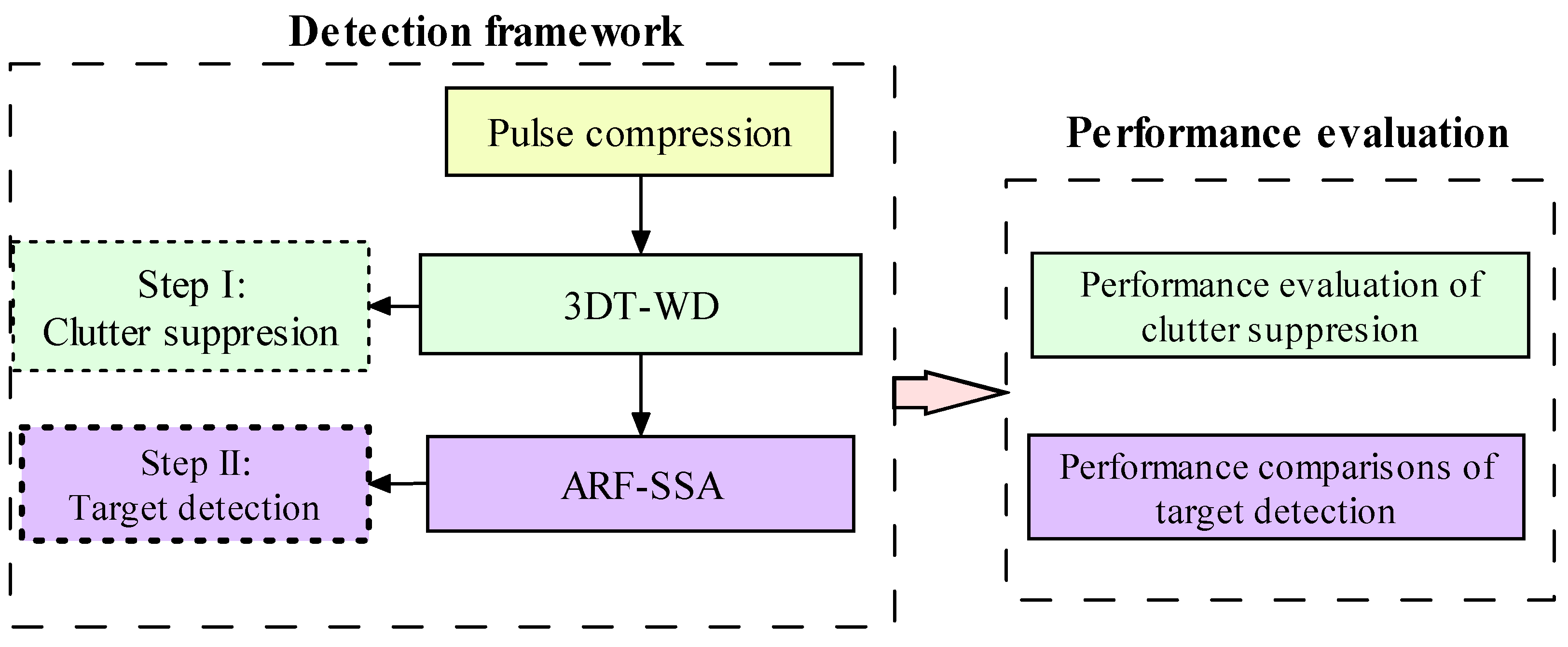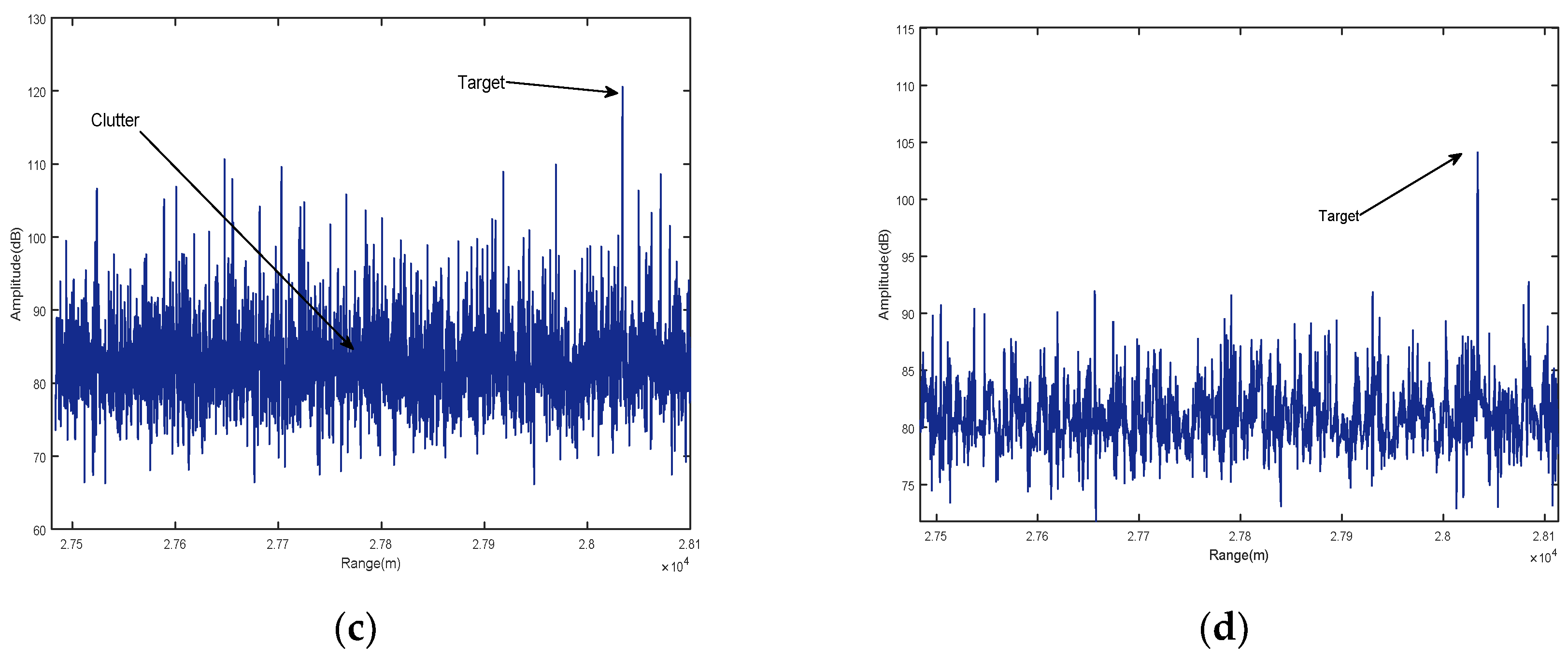In [24], based on the features of the returned signals in the time and frequency domains, a support vector machine (SVM) is implemented to detect small sea-surface targets. Motivated by STAP and machine learning technologies, we propose a two-step scheme by integrating the signal processing and machine learning techniques to improve the performance of detecting distributed targets in non-Gaussian noise, modeled as the sum of K-distributed clutter plus thermal noise. Firstly, the mixed method by combining 3DT space-time adaptive processing with wavelet denoising (3DT-WD) is utilized to improve the output signal-to-clutter plus-noise ratio before target detection. Second but more importantly, a novel detection method based on random forest optimized with the sparrow search algorithm (RF-SSA) is proposed. The experiment results show that the proposed RF-SSA can achieve better detection performance than several peer methods. The proposed RF-SSA framework is illustrated in Figure 1. The major innovations of this paper can be summarized as follows:

• The proposed RF-SSA is an adaptive detection method, which solves the unbalance between detection probability and efficiency of the traditional RF, without any prior knowledge.
• We tested if the 3DT-WD makes an improvement in the output signal-to-clutter plus-noise ratio (SCNR) and detection performance.
• Comprehensive analyses, including parameter determination, such as the number of decision trees of RF optimized by the SSA, together with the performance compared to the other related methods, are also evaluated.
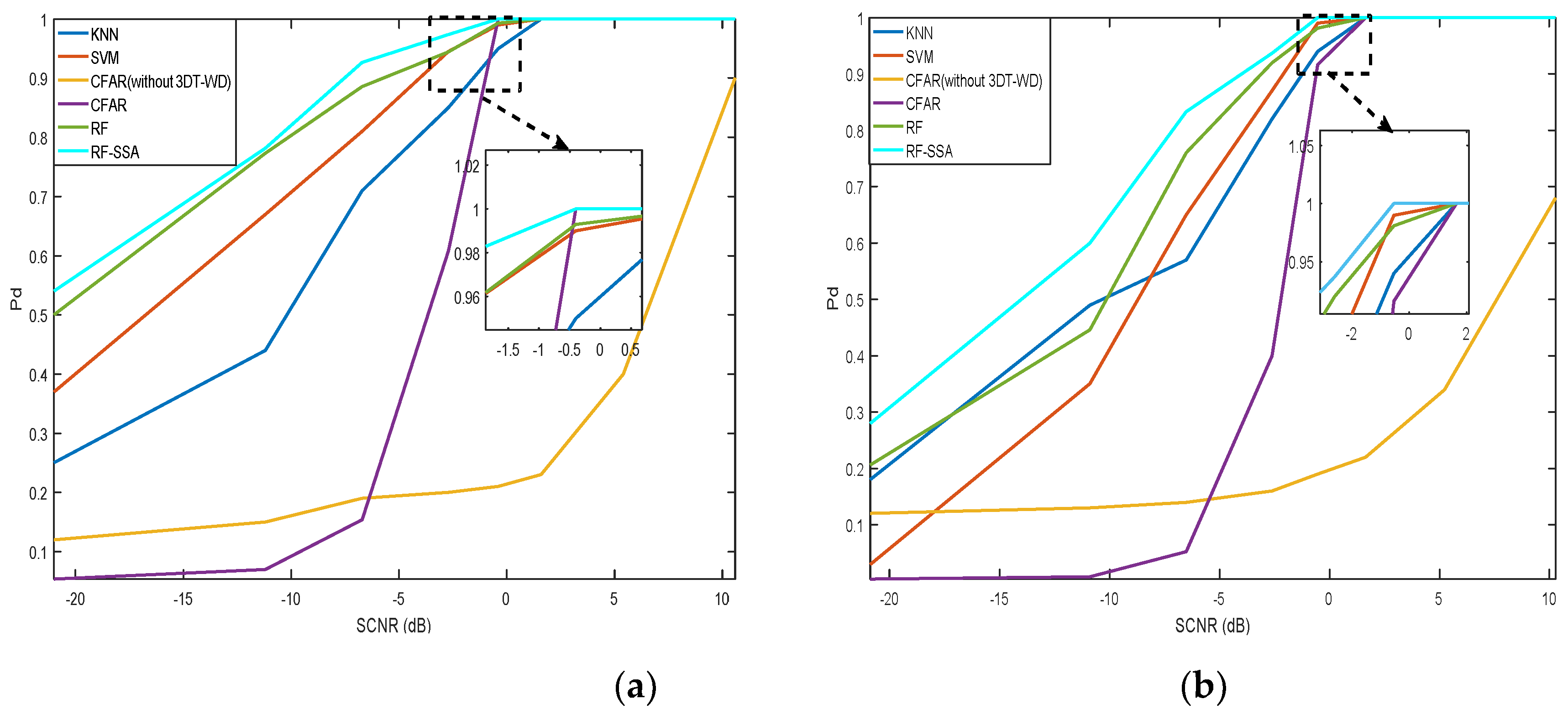
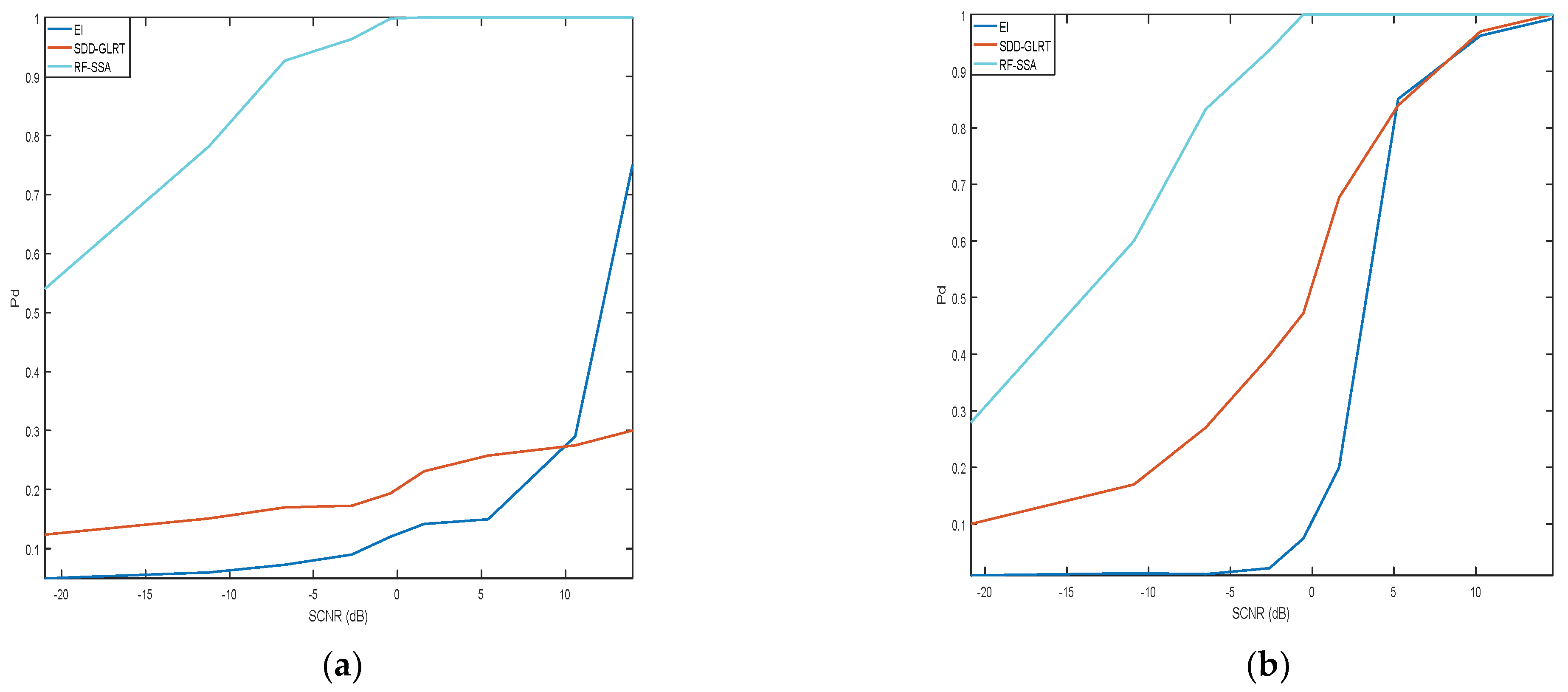
• The proposed RF-SSA can achieve better or more competitive performance in terms of detection probability and area under the receiver operating characteristic curve (AUC), compared to several peer methods. Additionally, the RF-SSA is more robust for the shape parameter of the clutter distribution compared to the scatterer density-dependent GLRT (SDD-GLRT) and energy integration (EI) detectors.

The main content of this paper is organized as follows. In Section 2, the detection problem is described. Then, in Section 3, the proposed detector is designed. In Section 4, numerical simulations are conducted for performance evaluation. Finally, Section 5 concludes this paper.

2. Problem Formulation

The target detection with an airborne radar system is carried out in this paper. It is assumed that received data are collected from the N-sensor radar system and the targets are completely contained within the received data. Radar returns $z\in {ℂ}^{NM\times 1}$ denote the space-time data in the cell under test, and M is the number of pulses in a coherent processing interval (CPI).

The distributed target detection problem can be expressed in the following binary hypothesis:

$$\{\begin{array}{l}{H}_0:z_t=c_t\begin{array}{ccc}+n_t,& & t=1,\dots ,D,D+1,\dots ,D+R\end{array}\\ H_1:\{\begin{array}{l}{z}_t=s_t+c_t+n_t,t=1,2,\dots ,D\\ z_t=c_t+n_t,\begin{array}{cc}& t=D+1,D+2,\dots ,D+R\end{array}\end{array}\end{array}$$

(1)

where the received data $z_t=s_t+c_t+n_t$ ($t=1,2,\dots ,D$) are called the primary data from the t-th radar distributed cell, and D is the number of range cells occupied by the target. $z_t=c_t+n_t$ ($t=D+1,\dots ,D+R$) are the second data from the t-th range cell. $s\in {ℂ}^{NM\times 1}$, $c\in {ℂ}^{NM\times 1}$, and $n\in {ℂ}^{NM\times 1}$ denote the target returns, clutter, and thermal noise, respectively. Specifically, $n_t$ ($t=1,\dots ,D+1,\dots ,D+R$) is modeled as zero-mean white Gaussian noise. $c_t=g_t{w}_t$ ($t=1,\dots ,D+1,\dots ,D+R$) can be modeled as K-distribution clutter, $g_t$ and $w_t$ are the texture and speckle parts of the clutter, respectively. $w_t$ follows a complex Gaussian distribution, with zero mean and speckle covariance matrix $R\in {ℂ}^{MN\times MN}$. The texture $g_t$ follows a Gamma distribution with scale parameter $\tilde{q}$ and shape parameter v, and it represents the characteristics of the observed scene. The probability density function (PDF) of the texture part $g_t$ is

$$f(g_t)=\frac{{\tilde{q}}^{-v}}{\Gamma (v)}{g}_{{}_t}^{v-1}{e}^{-{\tilde{q}}^{-1}{g}_t}(g_t\ge 0,v\ge 0,\tilde{q}\ge 0)$$

(2)

where $\Gamma (\cdot )$ is the gamma function.

PDF of clutter is given by

$$f_K(t;v,q)=\frac{2}{q\Gamma (v)}{(\frac{t}{q})}^{(v-1)/2}{\mathrm{K}}_{v-1}(2\sqrt{\frac{t}{q}})$$

(3)

where ${\mathrm{K}}_v(x)$ denotes a modified Bessel function of the second kind and shape parameter v can control the tails of the PDF, i.e., the clutter is locally Gaussian if shape parameter v + ∞.

3. Proposed Detector

In this section, we address the detection problem of distributed targets in non-Gaussian noise, modeled as the sum of K-distributed clutter plus thermal noise. First, 3DT-WD is utilized to realize clutter suppression, then, the RF-SSA is performed to decide between $H_0$ and $H_1$ in (1), which is the major contribution of step II. Finally, to further verify the effectiveness of the proposed RF-SSA, the performance evaluation based on the real radar data is operated. The framework of the proposed detector is summarized in Figure 1, and SCNR is denoted as follows:

$$\mathrm{SCNR}=\frac{1}{LM}{\displaystyle \sum _{m=1}^M(s_m}{)}^T{R}^{-1}(s_m)$$

(4)

where $L$ is the number of radar system channels, ${(\cdot )}^T$ denotes the Hermitian transpose, and $R$ is the interference covariance matrix.

3.1. Step I: 3DT-WD for Clutter Suppression

3.1.1. 3DT

The movement of the radar platform can result in a significant Doppler spread of clutter, which may obscure the Doppler information of the target. Therefore, the target cannot be distinguished from the clutter easily by only using the Doppler information. To solve this problem, STAP is derived by combining spatial azimuth information and Doppler information. However, DOFs of conventional STAP techniques are equal to DM (D is element number), which results in a great amount of training samples (between 2 and 5 times the number of DOFs of the processor) to estimate the clutter covariance matrix. In addition, those training data satisfy the identical independent distribution (IID) condition, which is often inadequate in heterogeneous environments. To maintain the performance of STAP methods with limited sample supports, some suboptimal STAP approaches are proposed. 3DT can greatly reduce DOFs of the radar system by linearly transforming the echo data with the full-dimensional into the data with a low-dimensional space, achieving a good compromise between the computational burden and interference suppression performance; thus, it is a priority algorithm in practical engineering applications.

The 3DT algorithm firstly transforms the received signals of each channel from the time domain to the Doppler domain through weighted fast Fourier transformation (FFT) and then combines the Doppler unit where the target is to be detected and its adjacent Doppler units for adaptive processing.

For the k-th Doppler unit, its reduced-dimension matrix can be expressed as

$$T_k=F_k\lambda \otimes I_N$$

(5)

where $F_k={\left(\begin{array}{llll}1& e^{-j\frac{2\pi }{M}(k-1)}& \dots & e^{-j\frac{2\pi }{M}(k-1)(M-1)}\\ 1& e^{-j\frac{2\pi }{M}k}& \dots & e^{-j\frac{2\pi }{M}k(M-1)}\\ 1& e^{-j\frac{2\pi }{M}(k+1)}& \dots & e^{-j\frac{2\pi }{M}(k+1)(M-1)}\end{array}\right)}_{3\times M}$ is the FFT transformation matrix, $\lambda =\left(\begin{array}{llll}{\lambda }_1& & & \\ & {\lambda }_2& & \\ & & \ddots & \\ & & & {\lambda }_M\end{array}\right)$ is the weight matrix, and ${\lambda }_1,{\lambda }_2,\dots ,{\lambda }_M$ is the weight coefficient.

After using the reduced-dimension matrix $T_k$, the received data corresponding to the k-th doppler unit, the target steering vector, and the noise covariance matrix become ${\tilde{z}}_k=T_{k}z$, ${\tilde{s}}_k=T_{k}s$, ${\tilde{R}}_k=T_{k}R{T}_k^H$, respectively.

The optimal weight vector of the k-th doppler unit to be detected can be written as

$${\tilde{w}}_k=\gamma {\tilde{R}}_k^{-1}{\tilde{s}}_k$$

(6)

As the noise and clutter characteristics are unknown, the covariance matrix in Equation (6) can be obtained by the following maximum likelihood estimate method:

$${\hat{\tilde{R}}}_k=\frac{1}{L}{\displaystyle \sum _{l=1}^L{\tilde{z}}_{k;l}{\tilde{z}}_{k;l}^H}$$

(7)

where L is the number of samples and ${\tilde{z}}_{k;l}$ represents the data from adjacent samples of the k-th Doppler unit, after using a reduced-dimension matrix $T_k$.

Based on the above analysis, it can be concluded that the DOFs of 3DT are much smaller than that of the full-dimensional STAP, i.e., it is reduced from MN to 3N, which greatly reduces the computational burden and the number of IID training samples.

In practice, the clutter suppression performance of conventional 3DT may be remarkably reduced when training samples do not satisfy the IID assumptions in heterogeneous environments. Wavelet transform has the ability of multi-resolution analysis, which is especially suitable for non-stationary signal processing. For noise reduction, wavelet transform is a reasonably effective method. Therefore, wavelet transform is introduced to improve SCNR.

3.1.2. Wavelet Denoising

Based on the wavelet basis function and threshold function, satisfactory denoising performance can be achieved. In general, wavelet denoising consists of three steps, as follows:

• Wavelet decomposition

After selecting a mother wavelet and determining the level of wavelet decomposition, the wavelet transform is applied to the input noisy signals.

2.

Wavelet threshold

Wavelet denoising is highly dependent on the threshold function. After wavelet decomposition, the wavelet approximation $a_{j,k}$ and detail coefficient $d_{j,k}$ are obtained. Then, the wavelet detail coefficient that involves the noise components can be filtered by the threshold. The threshold selection and refinement process mainly consist of general threshold, adaptive threshold, and wavelet packet threshold.

The wavelet packet threshold method carries out the next layer of decomposition for both low-frequency and high-frequency sub-bands of each layer of wavelet decomposition and has the capability of adaptive threshold processing at different scales, which makes the wavelet domain information more detailed with a low computing burden. Therefore, the wavelet packet-based threshold method is adopted in this paper.

3.

Wavelet reconstruction

By applying inverse wavelet transform on the modified coefficients, the recovery signal $\mathrm{y}(i)$ is obtained through the inverse DWT (IDWT).

$$\mathrm{y}(i)={\displaystyle \sum _k{a}_{{}_j{,}_k}{\varphi }_{j,k}(i)+{\displaystyle \sum _j{\displaystyle \sum _k{d}_j{}_{,k}{\psi }_{j,k}(i)}}}$$

(8)

where $a_{{}_j{,}_k}=\langle \mathrm{z}(i),{\varphi }_{j,k}(i)\rangle$, $d_j{}_{,k}=\langle z(i),{\psi }_{j,k}(i)\rangle$ and j is an arbitrary scale. $\varphi (i)$ and $\psi (i)$ are wavelet functions, and they provide the wavelet approximation coefficient and detail coefficient at scale j, respectively.

3DT-WD in step I is a straight-forward method to improve SCNR. In the following section, the RF-SSA is proposed to achieve the detection of distributed targets, which is the major contribution of step II.

3.2. Step II: RF-SSA for Target Detection

3.2.1. RF

As for the detection problem itself, identifying a target from interference can be considered a classification problem in nature. The RF is an ensemble learning approach, it has state-of-the-art classification performance and is insensitive to over-fitting, which makes it one of the most popular classifiers. It also consists of a large number of decision trees that are generated by the bootstrap sampling technique. At each node, the best split point of each decision tree is generated based on the selected feature subsets. One must note that feature subsets are randomly selected from the full features ($n\ll N_1$, n is the number of the selected features, N₁ is the number of all features) at each node of each base decision tree C_i (i = 1, 2, …, w, w is the number of the decision trees). Briefly, the RF is structured completely by combining the base decision trees, and the final classification results (0 and 1 denote hypotheses $H_0$ and hypotheses $H_1$, respectively) are determined by the votes of all the base decision trees. The classification process of the RF is shown in Figure 2.

3.2.2. RF-SSA

From the above analysis, the reasonable selection of the number of decision trees has a significant impact on the final classification accuracy. In general, the number of decision trees is obtained through iterative search or default parameter setting. However, the former is time-consuming with regard to learning tasks, and the latter hardly obtains optimal classification accuracy. To balance detection efficiency and accuracy, in this paper, SSA is implemented to adaptively compute the optimal number of the decision trees of RF.

SSA is a heuristic algorithm, derived from the theory of foraging behavior and anti-predation behavior of sparrows. It has the advantages of high optimization ability, few adjustment parameters, and fast convergence speed, having drawn important attention recently [25,26]. During the foraging search process, the sparrow colony is divided into two groups, discoverers and entrants. The discoverer has better fitness values and is responsible for searching foraging areas and directions for the entire sparrow population, while the entrants utilize the position of the discoverer to obtain food. At the same time, if the sparrows selected for investigation and early warning find the danger, and the alarm values are greater than the safety threshold, then the discoverers lead other sparrows to the safe place.

In the simulation experiment, the position of sparrows can be written as follows:

$$X= \left[\begin{array}{cccc}{x}_{1,1}& x_{1,2}& \cdots & x_{1,d}\\ x_{2,1}& x_{2,2}& \cdots & x_{2,d}\\ ⋮& ⋮& ⋮& ⋮\\ x_{q,1}& x_{q,2}& \cdots & x_{q,d}\end{array}\right]$$

(9)

where q is the number of the entire sparrows, and d is the dimension of the variables to be optimized.

During the iteration, the updated locations of discoverers can be described as follows:

$$X_{i,j}^{t+1}= \{\begin{array}{ll}{X}_{i,j}^t\cdot \exp (\frac{-i}{a\cdot I})& \mathrm{if} R_2<ST\\ X_{i,j}^t+Q\cdot B& \mathrm{if} R_2\ge ST\end{array}$$

(10)

where t indicates the current number of iterations, I is a constant, indicating the largest number of iterations and $a\in (0,1]$ is a random number. Q represents the normal distribution random number and B indicates a 1 × d matrix for which each element inside is 1. $R_2\in [0,1]$ is the alarm value and $ST\in [0.5,1]$ is the safety threshold.

When $R_2<ST$, it means that there are no predators in the neighborhood and then the discoverer continues to search for food; when $R_2\ge ST$, it means that there are some sparrows that have detected the predator, and then all sparrows immediately fly to other safe zones to search for food.

The updated locations of entrants can be described as follows:

$$X_{i,j}^{t+1}=\{\begin{array}{ll}Q\cdot \exp (\frac{X_{worst}^t-X_{i,j}^t}{i^2})& \mathrm{if} i>q/2\\ X_p^{t+1}+\frac{1}{d}{\displaystyle \sum _{j=1}^d(\mathrm{rand}(-1,1)\cdot }\left|X_{i,j}^t-X_p^{t+1}\right|)& \mathrm{otherwise}\end{array}$$

(11)

where t represents the current iteration number and $X_p^t$ and $X_{worst}^t$ represent the global best and worst positions at the t-th iteration, respectively.

When $i>q/2$, it means that the i-th entrant cannot obtain food and needs to change position to search for food. When $i\le q/2$, it means that the i-th entrant is near to $X_p^t$ and is randomly foraging around.

In general, the alerters account for 10% to 20% of the entire sparrow population, and its updated locations can be described as follows:

$$X_{i,j}^{t+1}=\{\begin{array}{ll}{X}_{best}^t+\beta \times \left|X_{i,j}^t-X_{best}^{t+1}\right|& \mathrm{if} f_i>f_g\\ X_{i,j}^t+K_1\times (\frac{\left|X_{i,j}^t-X_{worst}^{t+1}\right|}{(f_i-f_w)+\epsilon })& \mathrm{if} f_i=f_g\end{array}$$

(12)

where $\beta$ is a random value, subject to a normal distribution with a mean value of 0 and a variance of 1, and it can control the step size, $K_1\in [-1,1]$ indicates the moving direction of the sparrow population and $\epsilon$ is the smallest constant, which is used to avoid zero-division-error. $f_i$ is the fitness value of the i-th sparrow, $f_g$ and $f_w$ are the global best and worst fitness values of the current sparrow population, respectively.

The position of the discoverer is based on the minimum classification error rate $f^{\ast }$, which is the objective function in the simulation, and $f^{\ast }$ is denoted as follows:

$$f^{\ast }=1-\frac{TP}{TP+FP}$$

(13)

where TP is the true position, and FP is the false positive.

Based on the above analysis, the algorithm flow chart of the RF-SSA can be summarized in Figure 3.

4. Results and Analysis

4.1. Detection Performance Assessment on Simulated Data

To evaluate the performance of the proposed method, in this section, first, the effectiveness of 3DT-WD is verified, then performance evaluations for the proposed RF-SSA, the traditional RF, KNN [23], and SVM [24] are carried out. To further verify the effectiveness of the proposed RF-SSA, we also compare it with the detection performance of the SDD-GLRT and EI detectors.

4.1.1. Parameter Determination

We assume that the total energy of the target scatterers is evenly distributed among four range cells, and D = 83. The key radar parameters in the simulations are given in

Table 1. Parameters of radar.

Parameter	Value
Carrier frequency	10 GHz
Bandwidth	600 MHz
Range resolution	0.25 m
Pulse repetition interval	2 ms
Inter element spacing	0.015 m
Identical antenna elements	16
Number of pulses	16
Wavelength	0.03 m

. In step I, wavelet transform is based on Daubechies (db4) wavelet basis functions. In step II, we could yield 500 target samples and 1700 sea clutter samples, then, we randomly sample 70% data as the training set, and the remaining 30% are used as the test set. The parameter setting of the RF-SSA is as follows: the largest number of iterations I = 10, the initial number of sparrows is 10, and the number of discoverers accounts for 20% of the entire sparrow population, ST = 0.8, the number value range of the decision trees is set 1, 300, and the interval is set 5. For KNN, the number of neighbors is 5, and the leaf size is 10. For SVM, the radial basis function is adopted here, and the regularization parameter is 1.

In addition, the power of the Gaussian white noise is set according to CNR = 20 dB. The CNR is formulated as follows:

$$CNR=\frac{{\displaystyle {\sum }_{r=1}^R{\mathit{c}}_r^H{\mathit{c}}_r}}{R{\sigma }_n^2}$$

(14)

where ${\sigma }_n^2$ is the average power of the white Gaussian noise; $R$ denotes the number of range cells, and ${\mathit{c}}_r$ is the clutter in the r-th range cell.

The simulations are implemented on CPU AMD Ryzen 7 3700X@3.59 GHz 8-core and RAM Kingston FURY 16GB DDR4. The signal pre-processing algorithm (3DT-WD) in step I is carried out on Matlab2016 (a) software (Matlab 2016 is a commercial math software from MathWorks, Natick, MA, USA), and the proposed detection algorithm (RF-SSA) in step II is carried out on the PyCharm Community simulation platform, programming languages, Python3.7.

4.1.2. Performance Evaluation

First, the performance of conventional 3DT and the proposed 3DT-WD are tested, respectively, as shown in Figure 4. It can be observed from Figure 4a that since the linear frequency modulation (LFM) signals have a large gain in pulse compression, the radar can easily detect the target in Gaussian noise. The target is submerged when sea clutter enters the radar main lobe, failing target detection, as shown in Figure 4b. Then, the 3DT algorithm is utilized to suppress the clutter, as shown in Figure 4c and the target amplitude is only slightly higher than the clutter amplitude, which means it is still difficult to achieve the target detection. After using 3DT-WD, as shown in Figure 4d, it can be observed that the output SCNR is greatly improved, which verifies the effectiveness of 3DT-WD.

Then, we compare the RF-SSA with the traditional RF, wherein the number of decision trees is obtained through iterative searches to evaluate the detection efficiency, and the computational cost of the two methods is shown in

Table 2. Comparisons of average computational cost (v = 0.1).

SCNR/dB	−20.9	−11.2	−6.7	−2.7	−0.4	1.6	T/s
RF-SSA	83.3%	88.7%	95.1%	96.7%	99.8%	1	316.2
RF	82.8%	88.5%	94.9%	97.3%	99.5%	1	579.2

. The results show that the average detection accuracy of the RF-SSA is relatively close to the traditional RF with iterative searches, achieving the optimal detection accuracy rapidly within 10 iterations. More importantly, the average computational cost of the RF-SSA is greatly lower than the traditional RF with iterative searches, i.e., 316.2 and 519.2 s (v = 0.1), respectively, which demonstrates that the RF-SSA can greatly improve the detection efficiency.

Moreover, the performance of the RF-SSA is compared with that of the traditional RF with default parameters, KNN, SVM, and the CFAR and the detection results are shown in Figure 5. It can be observed that the RF-SSA can provide highly competitive results compared to the other algorithms, obtaining an up to 2-dB performance improvement, followed by the RF, SVM, KNN, and the CFAR method performs the worst. Combining the results in Table 2, the proposed RF-SSA can solve the unbalance between detection probability and efficiency of the traditional RF. Moreover, the detection probability of the proposed RF-SSA rises as v decreases. In addition, the performance of the CFAR is greatly improved after using 3DT-WD, which indicates that the 3DT-WD helps to improve the detection performance.

To evaluate the overall detection performance, we also compare the RF-SSA with the other algorithms in terms of AUC. As shown in

Table 3. Comparisons of AUC (v = 0.1).

SCNR/dB	−20.9	−11.2	−6.7	−2.7	−0.4	1.6
KNN	58.8%	62%	78.3%	84.3%	90.8%	99%
SVM	66.7%	81.8%	89.7%	96%	99.5%	1
RF	75.5%	86.7%	93.8%	97.1%	98.9%	1
RF-SSA	77.7%	88.2%	95%	99%	1	1

and

Table 4. Comparisons of AUC (v = 0.5).

SCNR/dB	−20.9	−10.9	−6.5	−2.6	−0.5	1.7
KNN	52.5%	53.3%	61.3%	69.3%	90.1%	95.3%
SVM	60.3%	70.4%	79.5%	93.2%	99.1%	1
RF	71.4%	76.6%	87%	95.8%	99.4%	1
RF-SSA	72.2%	81%	90%	97.8%	99.8%	1

, the RF-SSA is superior to the other methods, which also indicates that the proposed RF-SSA has a lower false alarm rate.

Finally, to further evaluate the effectiveness of the proposed method, the detection results of RF-SSA are compared with the SDD-GLRT and EI detectors, under the K-distributed clutter with the shape parameters v = 0.1 and v = 0.5. As we cannot obtain the detection probability P_d and the false alarm probability P_fa in closed form, the detection probability P_d for the SDD-GLRT and EI detectors are estimated based on the Monte Carlo technique. In the simulation, each P_fa and P_d are obtained via 10/P_fa and 1/P_fa independent Monte Carlo experiments. Specifically, P_fa is set to 10⁻⁴ and the key radar simulation parameters remain unchanged. As shown in Figure 6, it can be observed that the performance of the RF-SSA outperforms the SDD-GLRT and EI detectors, in particular the low SCNR cases. Moreover, the RF-SSA achieves more robust detection performance in heterogeneous environments, compared with the other two detectors.

4.2. Detection Performance Assessment on Real RadarData

This subsection is devoted to the performance assessment of the RF-SSA, KNN, and SVM, in terms of probability of detection (P_d), by exploiting real radar data using the Ku-band radar. More specifically, the key radar parameters are given in

Table 5. Parameters of real radar.

Parameter	Value
Carrier frequency	16 GHz
Bandwidth	64 MHz
Range resolution	2.34 m
Pulse repetition interval	24.8 ms
Wavelength	0.0187 m
Sampling rate	100 MHz

and the target echo is collected from three same angle reflector, which occupies 64 range cells (D = 63). Then, we could yield 2000 target samples and 7000 clutter samples, and the detection results with real data are shown in

Table 6. Comparisons of the detection probability.

Methods	Pd
	SCR = 5.7 dB	SCR = 7.9 dB	SCR = 10.5 dB
RF-SSA	80.7%	96%	99.3%
RF	78.7%	94.7%	98.7%
KNN	32.7%	73.3%	85.3%
SVM	44%	88%	96.7%

and

Table 7. Comparisons of AUC.

Methods	Pd
	SCR = 5.7 dB	SCR = 7.9 dB	SCR = 10.5 dB
RF-SSA	89%	97.5%	99.6%
RF	87.6%	96.6%	99%
KNN	65.8%	86.1%	92.7%
SVM	71.5%	93.5%	98.3%

. It should be noted that the parameter settings of the detection methods (RF-SSA, RF, KNN, and SVM) remain unchanged. In addition, since our focus is on the performance of the proposed RF-SSA, for simplicity, the signal pre-processing method (3DT-WD) is not used before target detection. The performance evaluation is carried out on the PyCharm Community simulation platform.

As shown in Table 6, it can be observed that the proposed RF-SSA outperforms the other three under different SCR situations. For example, the proposed RF-SSA improves the detection probability P_d by 1.3%, 22.7%, and 8% compared with the RF, KNN, and SVM, respectively, when SCR = 7.9 dB.

We further compare our RF-SSA with the other methods in terms of AUC in Table 7. It can be observed that, compared with the RF, KNN, and SVM, the proposed RF-SSA always works better under different SCR situations. For instance, the proposed RF-SSA improves the AUC values by 0.9%, 11.4% and 4% compared with the RF, KNN, and SVM, respectively, when SCR = 7.9 dB, which indicates that the proposed method has a lower false alarm rate.

Finally, we compare the detection performance of the proposed RF-SSA with that of the SDD-GLRT and EI detectors. For this experiment, the false alarm probability is set to be P_fa = 10⁻⁴. To evaluate the P_d and P_fa, 2000 target samples and 7000 clutter samples are used in the Monte Carlo experiments. Since the target occupies 64 range cells (D = 63), the range of the detection window for the SDD-GLRT and EI detectors is set to (40, 100). The detection results with real data are shown in

Table 8. Comparisons of the detection probability.

Methods	Pd
	SCR = 5.7 dB	SCR = 7.9 dB	SCR = 10.5 dB
RF-SSA	80.7%	96%	99.3%
EI	80.4%	89.1%	96.3%
SDD-GLRT	81.9%	89.6%	96.8%

. The proposed RF-SSA outperforms the other two detectors, and the EI detector is worse than the SDD-GLRT detector. For instance, the proposed RF-SSA improves the detection probability P_d by 6.9%, and 6.4% compared with the EI, and SDD-GLRT detectors, respectively, when SCR = 7.9 dB.

5. Conclusions and Future Work

In this paper, we propose a novel RF-SSA to detect distributed targets in non-Gaussian noise, modeled as the sum of K-distributed clutter plus thermal noise. The proposed RF-SSA can adaptively solve the unbalance problems between detection probability and efficiency of the traditional RF, without any prior knowledge. Moreover, the experimental results have verified that our proposed method outperforms several existing methods under different clutter environments.

Although the proposed method can greatly improve detection efficiency with respect to the traditional RF, it is unable to achieve real-time target detection. To alleviate computation load, feature extraction methods, for instance t-distributed random neighborhood embedding, principal component analysis, maximal information coefficient, etc., can be used before target detection.

In this paper, we assume that the problem of detecting distributed targets is investigated under a fixed CNR. However, the CNR in realistic scenarios is various and uncertain. Thus, future work will examine the performance of the proposed detector in practical application.

References

1. Shen, S.; Nie, X.; Tang, L.; Bai, Y.; Zhang, X.; Li, L.; Ben, D. An Improved Coherent Integration Method for Wideband Radar Based on Two-Dimensional Frequency Correction. Electronics 2020, 9, 840. [Google Scholar] [CrossRef]
2. Wang, P.; Li, H.; Kavala, T.R.; Himed, B. Generalised Parametric Rao Test for Multi-Channel Adaptive Detection of Range-Spread Targets. IET Signal Process. 2012, 6, 404. [Google Scholar] [CrossRef] [Green Version]
3. Liu, J.; Chen, J.J.; Li, J.J. Persymmetric Adaptive Detection of Distributed Targets with Unknown Steering Vectors. IEEE Trans. Signal Process. 2020, 68, 4123–4134. [Google Scholar] [CrossRef]
4. Liu, W.J.; Liu, J.; Gao, Y.C. Multichannel Signal Detection in Interference and Noise When Signal Mismatch Happens. Signal Process. 2020, 166, 107268. [Google Scholar] [CrossRef]
5. Zuo, L.; Li, M.; Zhang, X.W.; Zhang, P. CFAR Detection of Range-Spread Targets Based on the Time–Frequency Decomposition Feature of Two Adjacent Returned Signals. IEEE Trans. Signal Process. 2013, 61, 6307–6319. [Google Scholar] [CrossRef]
6. Yang, X.L.; Wen, G.J.; Ma, C.H.; Hui, B.W.; Ding, B.Y.; Zhang, Y.H. CFAR Detection of Moving Range-Spread Target in White Gaussian Noise Using Waveform Contrast. IEEE Geosci. Remote Sens. Lett. 2016, 13, 282–286. [Google Scholar] [CrossRef]
7. Conte, E.; Maio, A.D.; Ricci, G. CFAR Detection of Distributed Targets in Non-Gaussian Disturbance. IEEE Trans. Signal Process. 2014, 62, 331–342. [Google Scholar] [CrossRef]
8. Liu, J.; Liu, W.J.; Tang, B. Distributed Target Detection Exploiting Persymmetry in Gaussian Clutter. IEEE Trans. Signal Process. 2019, 67, 1022–1033. [Google Scholar] [CrossRef]
9. Xiao, L.; Liu, Y.; Huang, T.; Liu, X.; Wang, X. Distributed Target Detection with Partial Observation. IEEE Trans. Signal Process. 2018, 66, 1551–1565. [Google Scholar] [CrossRef]
10. Yang, Y.; Xiao, S.P.; Wang, X.S.; Li, Y.Z. Non-Coherent Radar Detection Probability for Correlated Gamma Fluctuating Targets in K-Distributed Clutter. IEEE Access 2018, 6, 3824–3827. [Google Scholar] [CrossRef]
11. Xue, J.; Xu, S.W.; Liu, J.; Shui, P.L. Model for Non-Gaussian Sea Clutter Amplitudes Using Generalized Inverse Gaussian Texture. IEEE Trans. Geosci. Remote Sens. 2019, 16, 892–896. [Google Scholar] [CrossRef]
12. Abramovich, Y.I.; Besson, O. Fluctuating Target Detection in Fluctuating K-Distributed Clutter. IEEE Signal Process. Lett. 2015, 22, 1791–1795. [Google Scholar] [CrossRef] [Green Version]
13. Jian, T.; He, Y.; Su, F.; Qu, C. Adaptive Range-Spread Target Detection Based on Modified Generalised Likelihood Ratio Test in Non-Gaussian Clutter. IET Radar Sonar Navig. 2011, 5, 970–977. [Google Scholar] [CrossRef] [Green Version]
14. Xiao, L.; Li, H.B.; Liu, Y.M.; Wang, X.Q. Distributed Target Detection Based on The Volume Cross-Correlation Function. IEEE Signal Process. Lett. 2018, 25, 1785–1789. [Google Scholar] [CrossRef]
15. Besson, O.; Tourneret, J.Y.; Bidon, S. Knowledge-Aided Bayesian Detection in Heterogeneous Environments. IEEE Signal Process. Lett. 2007, 14, 355–358. [Google Scholar] [CrossRef] [Green Version]
16. Besson, O.; Bidon, S.; Tourneret, J.Y. Covariance Matrix Estimation with Heterogeneous Samples. IEEE Trans. Signal Process. 2008, 56, 909–920. [Google Scholar] [CrossRef] [Green Version]
17. Jiang, Z.Z.; He, Y.; Li, G.; Zhang, X.P. Robust STAP Detection Based on Volume Cross-Correlation Function in Heterogeneous Environments. IEEE Geosci. Remote Sens. Lett. 2022, 19, 8000705. [Google Scholar] [CrossRef]
18. Cao, Z.H.; Fang, W.W.; Song, Y.Y. DNN-Based Peak Sequence Classification CFAR Detection Algorithm for High-Resolution FMCW Rada. IEEE Trans. Geosci. Remote Sens. 2022, 60, 5106115. [Google Scholar] [CrossRef]
19. Carrera, E.V.; Lara, F.; Ortiz, M. Target detection Using Radar Processors Based on Machine Learning. In Proceedings of the 2020 IEEE ANDESCON, Quito, Ecuador, 13–16 October 2020. [Google Scholar]
20. Rizvi, S.M.D.; Ahmad, S.; Khan, K. Deep Learning Approach for Fixed and Rotary-Wing Target Detection and Classification in Radars. IEEE Aerosp. Electron. Syst. Mag. 2022, 37, 32–42. [Google Scholar] [CrossRef]
21. Akhtar, J.; Olsen, K.E. A Neural Network Target Detector with Partial CA-CFAR Supervised Training. In Proceedings of the IEEE International Conference on Radar, Brisbane, Australia, 27–31 August 2018; pp. 1–6. [Google Scholar]
22. Dong, L.F.; Du, H.Q.; Mao, F.J. Very High Resolution Remote Sensing Imagery Classification Using A Fusion of Random Forest and Deep Learning Technique—Subtropical Area for Example. IEEE J. Sel. Top. Appl. Earth Obs. Remote Sens. 2020, 13, 113–128. [Google Scholar] [CrossRef]
23. Coluccia, A.; Fascista, A.; Ricci, G. A K-Nearest Neighbors Approach to the Design of Radar Detectors. Signal Process. 2020, 174, 107609. [Google Scholar] [CrossRef]
24. Li, Y.; Xie, P.C.; Tang, Z.S.; Jiang, T.; Qi, P.H. SVM-Based Sea-Surface Small Target Detection: A False-Alarm-Rate-Controllable Approach. IEEE Geosci. Remote Sens. Lett. 2019, 16, 1225–1229. [Google Scholar] [CrossRef] [Green Version]
25. Xue, J.; Shen, B. A Novel Swarm Intelligence Optimization Approach: Sparrow Search Algorithm. Syst. Sci. Control Eng. 2020, 8, 22–34. [Google Scholar] [CrossRef]
26. Yuan, J.H.; Zhao, Z.W.; Liu, Y.P. DMPPT Control of Photovoltaic Microgrid Based on Improved Sparrow Search Algorithm. IEEE Access 2021, 9, 16623–16629. [Google Scholar] [CrossRef]
Figure 1. An overview of the proposed method architecture.
Electronics 11 02319 g001
Figure 2. Basic structure of the random forest classifier.
Electronics 11 02319 g002
Figure 3. Algorithm flow chart of RF-SSA.
Electronics 11 02319 g003
Figure 4. The simulated results of the clutter suppression: (a) echo after pulse compression (Gaussian noise alone); (b) echo after pulse compression (clutter and internal noise; (c) echo after 3DT; (d) echo after 3DT-WD.
Electronics 11 02319 g004aElectronics 11 02319 g004b
Figure 5. Detection performance comparisons of different detectors: (a) v = 0.1; (b) v = 0.5.
Electronics 11 02319 g005
Figure 6. Detection performance comparisons of different detectors: (a) v = 0.1; (b) v = 0.5.
Electronics 11 02319 g006