
WeaveNet: Solution for Variable Input Sparsity Depth Completion


1
Aptiv Services Poland S.A., 30-399 Cracow, Poland
2
Faculty of Electrical Engineering, Automatics, Computer Science, and Biomedical Engineering, AGH University of Science and Technology, 30-059 Cracow, Poland
Electronics 2022, 11(14), 2222; https://doi.org/10.3390/electronics11142222
Submission received: 12 May 2022
/
Revised: 22 June 2022
/
Accepted: 22 June 2022
/
Published: 16 July 2022
(This article belongs to the Special Issue IoT for Intelligent Transportation Systems)
Abstract
:LIDARs produce depth measurements, which are relatively sparse when compared with cameras. Current state-of-the-art solutions for increasing the density of LIDAR-derived depth maps rely on training the models for specific input measurement density. This assumption can easily be violated. The goal of this work was to develop a solution capable of producing reasonably accurate depth predictions while using input with a very wide range of depth information densities. To that end, we defined a WeaveBlock capable of efficiently propagating depth information. To achieve this goal, WeaveBlocks utilize long and narrow horizontal and vertical convolution kernels together with MobileNet-inspired pointwise convolutions serving as computational kernels. In this paper, we present the WeaveNet architecture for guided (LIDAR and camera) and unguided (LIDAR only) depth completion as well as a non-standard network training procedure. We present the results of the network on the KITTI test and validation sets. We analyze the network performance at various levels of input sparsity by randomly removing between 0% and 99% of the LIDAR points from the network inputs, and in each case, we obtain reasonable quality output. Additionally, we show that our trained network weights can easily be reused with a different LIDAR sensor.
1. Introduction
Even high quality LIDARs used as depth sensors in automotive sector provide relatively low output density when compared to cameras. This can be easily observed in the KITTI dataset [1,2], one of the leading datasets related to perception in automotive settings. Velodyne HDL-64E LIDAR, whose output is provided in the KITTI dataset, produces approximately 20,000 detections in the field of view of the front camera, while the camera itself provides an image with 465,750 pixels (375 × 1242). One problem with such disparity in the input density is that early fusion of data from the camera and LIDAR in the camera plane requires interpolation of the depth information to fill in the gaps between sparse measurements. Another disadvantage of sparse and irregularly spaced depth predictions is that processing of LIDAR pointclouds requires more complicated neural network designs, such as PointNet [3] or VoxelNet [4], rather than simpler 2D convolutional networks that can be utilized on camera data. Finally, the most obvious problem with sparse LIDAR data is that they might not provide resolution high enough for the downstream processing algorithms to recognize fine details of the scene.
The field of depth completion deals with transforming the sparse LIDAR output into a dense depth map. In 2017, Uhrig et al. [1] published the KITTI Depth Completion dataset together with a seminal work on sparsity invariant convolutions. Since then, the field of LIDAR depth completion for automotive application has flourished, with the works submitted to the KITTI Depth Completion challenge [1] being the de facto state of the art. Almost all of the published works (e.g., [1,5,6,7,8,9,10]) deal exclusively with the default input sparsity (the input detection density of a Velodyne HDL-64E LIDAR). The works of Cheng, Ma and Yan [11,12,13] are notable exceptions. Assuming relatively constant input density is fine when operating on data collected using a high quality LIDAR in perfect weather conditions. Unfortunately, this assumption does not hold in real-life scenarios. For example, the density of LIDAR measurements can drop sharply in fog or heavy rain. In the case of a cheap LIDAR sensor and big differences in reflectance of objects surrounding the car, the situation becomes even more problematic—the measurement density can vary between different regions of the same frame.
Automotive systems relying on a depth completion module must stay robust when faced with changing weather conditions or scenes with objects of differing reflectance. Therefore, we believe that it is crucial to explore depth completion in a setting with a highly variable input density. It was our main motivation to create WeaveNet, a neural network designed to use one set of trained weights to perform depth completion over 2 orders of magnitude of input densities (200 to 20,000 of measurements in field of view (FOV)).
2. Related Work
2.1. Methods Based on Sparsity Invariant Convolutions
Uhrig et al. [1] published the KITTI depth completion dataset together with the definition of the sparsity invariant convolutions. The point behind the KITTI depth completion dataset is to provide a way to train and test models capable of transforming sparse depth measurements into a dense depth map. This dataset consists of 93 k frames, where each frame consists of a camera image, sparse depth data obtained by projecting the lidar pointcloud onto the camera plane and a semi-dense depth annotation on the camera plane. The semi-dense depth annotations were produced by accumulating 11 LIDAR scans and subsequently removing outliers (such as the outliers related to moving objects) by comparing the accumulated LIDAR data points to the depth map obtained using stereovision. The sparsity invariant convolutions [1] are a method to perform 2D convolutions on an input with variable sparsity. This is achieved by utilizing a mask which contains 1 s for valid input pixels (e.g., pixels where a LIDAR point is projected) and 0 s for invalid pixels. Before performing a convolution, the input is multiplied (pixelwise) by the validity mask. After performing the convolution (but before adding bias), the output is normalized by dividing it by the fraction of the valid pixels that were used to compute it. The mask is propagated in such a way that a pixel is considered valid if and only if at least one valid pixel was used to compute it. Using the notation from [1], the result of the convolution with kernel at the position is:
and the value of validity mask is propagated according to:
where x denotes the array of pixel values at the previous layer, o denotes the array storing information whether the pixel was valid in the previous layer (1 if it was valid, 0 if it was not), w denotes the array storing information about convolutional weights and b is the bias.
Huang et al. [5] performed the task of depth completion using an encoder-decoder, hourglass-style network utilizing sparsity invariant convolutions. To that end, they introduced sparsity invariant averaging and sparsity invariant upsampling. These are operations that enable a network to perform averaging and upsampling in a manner consistent with the sparsity invariant framework (and define the way in which validity masks should be propagated).
Eldesokey et al. [6] significantly expanded on the sparsity invariant convolution framework by lifting the requirement that the validity mask is binary. Instead, they allowed the confidence mask to take values between 0 and 1. Additionally, they restricted the convolutional weights to be non-negative and interpreted them as affinity between different pixels. Hence, the propagated depth for a specific pixel is an average of depths from neighboring pixels weighted by their affinities. They propagated the confidence for a specific pixel, making it an average of the confidences of neighboring pixels, weighted by their respective affinities. Eldesokey et al. [6] found it necessary to use a loss function which aims to maximize confidence as part of the training procedure.
Yan et al. [13] utilized an encoder-decoder hourglass-style network to produce dense depth output. They used separate yet identical encoders for image data and LIDAR data. Interestingly, both the LIDAR encoder and image encoder used sparsity invariant convolutions, together with masks generated using LIDAR datapoints (albeit the mask for the image encoder switches each zero to one and each one to zero). Yan et al. [13] provided an ablation analysis of the performance of the network when it was fed with data sparser than usual; however, they decreased the data density at most 4 times.
2.2. Methods Not Based on Sparsity Invariant Convolutions
Many of the best-performing methods for guided depth completion borrow heavily from the convolutional spatial propagation network (CSPN) by Cheng et al. [14], which was itself influenced by the non-depth completion work of Liu et al. [15]. Cheng’s neural network consisted of a conventional encoder-decoder network and an iterative depth propagation layer. The outputs of the encoder-decoder network were initial depth prediction and affinities to other pixels. The affinities between pixels were used as convolutional weights to propagate depth information. The values of affinities used when propagating depth information to a particular pixel were normalized, so that the sum of their absolute values equaled 1. The depth propagation step was performed iteratively. In their next paper [11], Cheng et al. defined a CSPN++ block that improved upon CSPN by making the number of propagation step iterations and size of the kernel used during the propagation step dependent on the input (in a learnable way).
The work of Park et al. [8] used a very similar approach, but introduced pixelwise confidence and relaxed constraints on affinity normalization. In the case of Park’s network, the outpust of the encoder-decoder network were the initial depth prediction, affinities to other pixels and, additionally, the pixelwise confidence. The iterative depth propagation layer performed depth propagation by using affinities and pixelwise confidence. The affinities between pixels multiplied by pixelwise confidenceweare used as convolutional weights to propagate depth information. The sum of the absolute values of affinities used when propagating depth information to a particular pixel was constrained to be no greater than 1. Unlike in the work of Eldesokey et al. [6], Park did not use confidence when calculating loss function.
The method developed by Tang et al. [9] focused on effectively utilizing the RGB input to propagate the sparse depth information. To that end, they used a vision encoder, which output convolutional weights that were later used by the part of the network processing sparse depth.
The work of Chen et al. [7] showed a different path to depth completion. Their network utilized 2 processing streams—a 2D stream in which LIDAR and RGB data were processed using conventional 2D convolution and a 3D processing stream in which they utilized 3D continuous convolutions, developed by Wang et al. [16]. As Chen et al. [7] pointed out in their work, the LIDAR points close together on the 2D projection can be far away in 3D space, and therefore, utilizing both 2D and 3D processing allows for a much better feature extraction process.
Qiu et al. [10] introduced a network that utilized a conventional processing stream that directly output the dense depth information and an alternative stream which produced surface normals as an intermediate step towards outputting depth prediction. The final depth prediction was a learnable weighted average of the previous two outputs. The interesting part of work performed by Qiu et al. [10] is that they used a synthetic dataset obtained using the Carla simulator [17] to pretrain the network on the task of surface normal prediction.
The work of Ma et al. [12] used a conventional encoder-decoder hourglass-style network (wherein the depth and image data are fused at the beginning of the encoder). The most important contribution of this work was that it introduced a self-supervised way to train a depth completion network. Ma et al. [12] introduced a training process utilizing spatio-temporal properties of consecutive LIDAR and image frames to train the network without semi-dense annotations. Specifically, they utilized a loss function taking into account depth prediction consistency with depth measurement at a specific pixel, photometric loss connected to image warping between consecutive frames and a smoothness term that penalized second order derivatives in the depth prediction. Notably, Ma et al. provided an ablation analysis of the performance of the network when it was fed with data that were sparser than usual.
3. Our Method
3.1. WeaveBlock
The main idea behind sparsity invariant convolutions [1] was that the network can produce a valid depth output for a particular picture only if at least one valid depth input pixel was used in the calculations. It follows that in order to process very sparse depth input, it is necessary to allow easy flow of information between pixels located far away from each other. In our network, this is achieved by utilizing WeaveBlocks. The main inspirations for the WeaveBlock design were sparsity invariant convolutions [1], and the general structure was loosely inspired by the depthwise separable convolutions in MobileNet [18]. Each WeaveBlock consists of the following elements:
- A pointwise convolution with a small number of channels;
- A sparsity invariant convolution with a long and narrow vertical kernel and a small number of channels;
- A pointwise convolution with a large number of channels;
- A pointwise convolution with a small number of channels;
- A sparsity invariant convolution with a long and narrow horizontal kernel and a small number of channels;
- A pointwise convolution with a large number of channels.
All mentioned convolutions use rectified linear unit (ReLU) [19] activation. In the case of the network whose results are presented in this article, the small number of channels was set to 12, the large number of channels was set to 128, and the long and narrow convolutional kernels were in the shapes 31 × 1 and 1 × 31.
The design of the WeaveBlock achieves the goal of propagating the depth information at a big distance (15 pixels in each direction). Additionally, it enables the network to perform more complicated computations utilizing 128 channels of pointwise convolutions while also being reasonably frugal with resources—please note that when computations are performed in kernels bigger than 1 × 1, the number of channels and number of channels in preceding layer is small.
3.2. Unguided WeaveNet Architecture
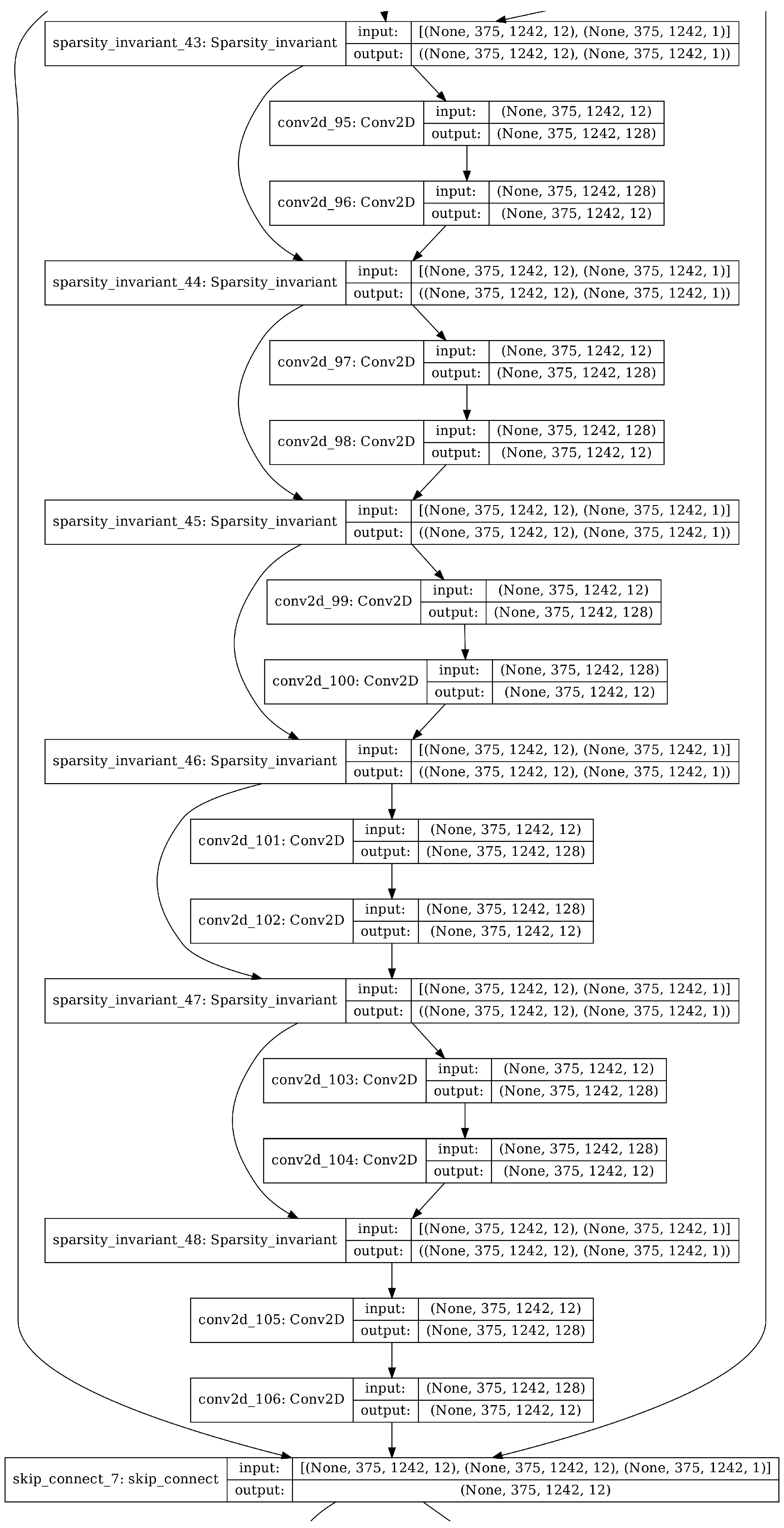
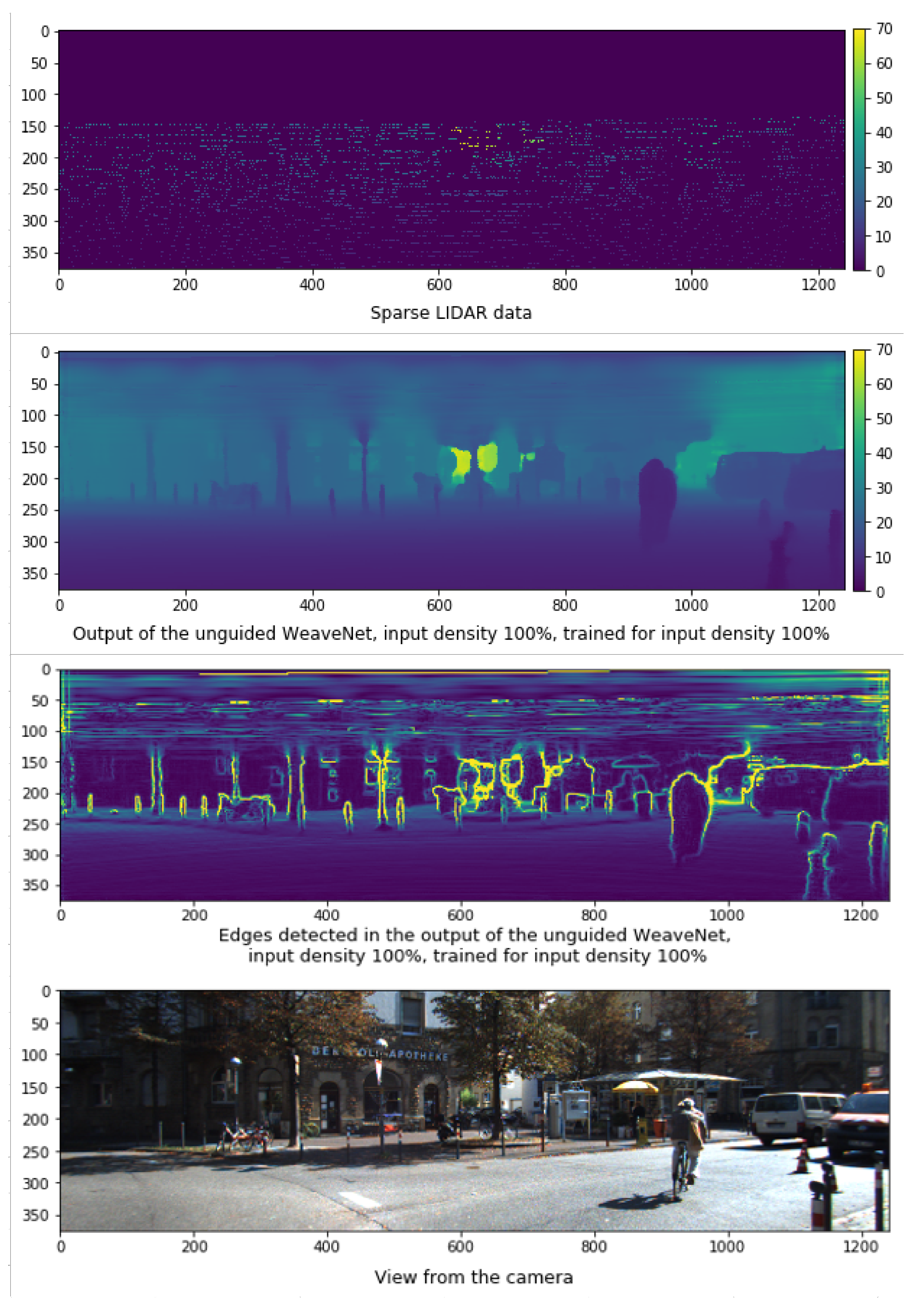
The unguided version of the WeaveNet architecture follows a simple, modular structure. Inside the network, WeaveBlocks are grouped in groups of 3, forming a single residual block. A schematic representation of a residual block containing 3 WeaveBlocks is presented in Figure 1. The residual blocks are wrapped in an averaging skip connection implemented similarly as in Huang’s sparsity invariant averaging [5]. The network consists of 5 identical residual blocks without any upsampling or downsampling—the network processing always happens at input and output resolution. The results obtained using the unguided WeaveNet, together with the corresponding LIDAR input and camera image, are presented in Figure 2. In the same figure, the edges in the output of the network are also shown to demonstrate the capability of the network to accurately represent fine details.
The unguided version of the network is the main part of this work. The guided version of the network does not contain significant improvements of its own and was prepared only to make the results obtained using WeaveNet comparable to other, guided solutions used in the KITTI depth completion task.
3.3. Guided WeaveNet Architecture
The RGB-guided version of the network utilizes the unguided architecture to preprocess the LIDAR depth information. The RGB data are preprocessed using a MobileNet [18]-inspired convolutional network, where a single functional convolution consists of:
- A pointwise convolution with a small number of channels;
- A 3 × 3 convolution with a small number of channels;
- A pointwise convolution with a large number of channels.
All mentioned convolutions use ReLU activation. The small number of channels for this subnetwork was set to 16, and the large number of channels was set to 128. A set of 3 such convolutions makes one residual block. In the beginning of a residual block, there is also an additional pointwise convolution with a small number of channels. There are also 2 batch-normalizing layers (after the first pointwise convolution and at the end of the residual block). The skip connection is implemented via concatenation of the outputs of the batch normalization layers. Please note that the concatenation input consists of 16 channels from the front of the block and 128 channels from the end of the block. We believe that such a network structure forces the model to compress the already-learned features to a small channel space while allowing for processing of the new features in a larger channel space. The vision preprocessing network consists of 3 such residual blocks and ends with a 1 channel convolution.
The preprocessed data from LIDAR and camera are concatenated; for both subnetworks, their ultimate and penultimate layer outputs are concatenated. Please note that this concatenation uses many more channels from the camera preprocessing (129 channels) than from LIDAR preprocessing (13 channels); we found it necessary for the network to extract useful camera features.
The fused data is processed by an aggregator network that is nearly identical to the vision preprocessing network; the only difference is that the aggregator network does not include batch normalization layers.
3.4. Notes on the Input and Output Modality
An important feature of unguided depth completion is that the inputs and outputs have the same modality—the distance to the nearest obstacle projected on the camera plane. Therefore, it is possible that inside the network, the information is also processed in the form of depth information rather than abstract channels. In such a case, it would be possible that the network weights are just a learnable way to interpolate between valid measurements. In fact, the good results in Eldesokey’s work on propagating confidence information in convolutional neural networks [6] may suggest that. Their method of depth completion achieved competitive results on the KITTI depth completion challenge while effectively restricting the convolutional weights to be non-negative. During the work on designing our depth completion network, we found several indications consistent with the possibility that the channels in the middle of the network are not abstract, but rather consistently represent depth.
- We found that using batch normalization in the LIDAR processing stream leads to greatly inferior results.
- We performed experiments using the same network architecture and activation functions other than ReLU. We found that using activation functions whose output may be negative such as Swish [20] and exponential linear unit (ELU) [21] leads to worse performance in the depth completion task than simple ReLU.
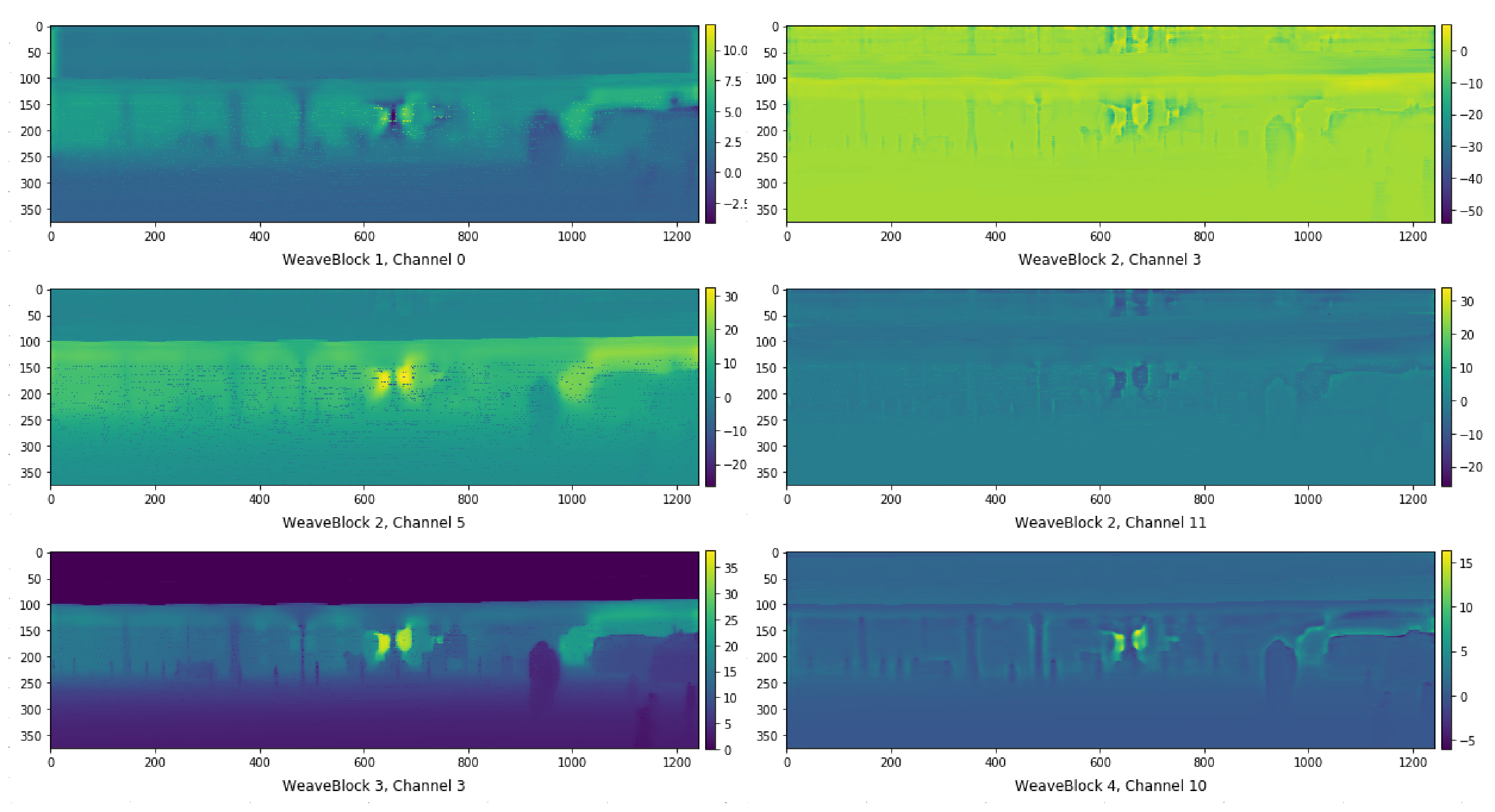
Such results are consistent with the possibility that at least some of the channels in intermediate layers of the network are directly representing depth. In fact, when examining the output of each residual block, we found that there are only 2 types of channels—channels whose output represents depth (up to an affine transformation) and channels whose output represents offsets at object edges. Example channels are shown in Figure 3.
3.5. Training Process
In this paper, we present 3 distinct versions of WeaveNet. Architecturally, they are equivalent, but they differ in terms of how they were trained:
- The first version was trained in a standard way (utilizing two training phases: pretraining and standard input density training).
- The second version was trained using universal sparsity training, which consisted of three training phases: pretraining, standard input density training and a variable input sparsity training.
- The third version was trained in a four phase specific sparsity training (pretraining, standard input density training, variable input sparsity training and a final phase of retraining the network at a specific input sparsity).
The full training procedure for the specific sparsity unguided version of the network was conducted in 4 distinct phases:
- A pretraining phase, during which instead of using LIDAR pointcloud as the input of the network, the network was fed with semi-dense depth labels. To be exact, the network was fed with KITTI Depth Completion labels with 50% of pixels masked with zeros. The pretraining phase was relatively short—only one epoch, utilizing approximately 20% of training set frames. This phase was performed using 10−3 learning rate. We found that this short pretraining phase greatly increases the speed of convergence in the future phases;
- The main training phase, during which the network was fed standard sparse input. This phase lasted 30 epochs. The optimizer learning rate was decreased from 10−3 to 10−4, then to 10−5, and finally to 10−6 during this phase. We found it beneficial to apply additive, normally distributed noise to the network weights during this phase of training (approach closer examined in [22]);
- The variable sparsity training phase. During this phase, the network was fed with input for which between 0% and 99.2% of the standard sparse input was masked with zeros. For a particular frame, the input density (i.e., the number of pixels that were not masked with zeros) was randomly sampled according to a formula:where and are the lowest (0.008) and highest (1.0) possible density levels, respectively, and is a random variable sampled uniformly between and .Such a sampling method achieves the goal that the probability of sampling a number from the interval and the probability of sampling a number from the interval is equal if and only if . This phase lasted 10 epochs and was performed with a 10−6 learning rate;
- The fixed sparsity training phase. The goal of the last training phase was to train the network at the target data sparsity (50% masked pixels, 75% masked pixels, 90% masked pixels, 95% masked pixels and 99% masked pixels). This phase lasted 2 epochs for each version of the network for a particular sparsity and was performed with a 10−6 learning rate.
For the training of the RGB-guided network, the weights obtained from training the unguided version for the first 2 phases were used as the starting weights of the LIDAR encoder. Additionally, 2 extra phases were employed after phase 2 and before phases 3 and 4:
- The RGB-encoder training phase. During this phase the weights of the LIDAR encoder were frozen. This phase lasted 10 epochs. The optimizer learning rate was decreased from 10−4 to 10−5 and finally to 10−6 during this phase;
- The joint training phase. During this phase the whole network was trained (no weights were frozen). This phase lasted 10 epochs and was performed with a 10−6 learning rate.
Huber loss was utilized during the entirety of training. The loss was quadratic for errors smaller than 5 m and linear for errors greater than 5 m. The whole training was performed using Adam [23] optimizer.
4. Experiments
4.1. Results on Standard Input Density
In this section, we present how WeaveNet compares to other guided and unguided solutions available in the literature (on the basis of root-mean-square error (RMSE) and mean absolute error (MAE)). All comparisons are based on the results on the KITTI validation set.
The RGB-guided version of WeaveNet is reasonably close to the state of the art in terms of MAE in the task of guided depth completion (Table 1). The RGB-guided version of WeaveNet is significantly worse than current state of the art RGB-guided depth completion solutions in terms of RMSE (Table 1). It should be noted that as of today, the solutions not relying on sparsity invariant convolutions seem to be significantly better at the task of guided depth completion.
Unguided WeaveNet achieves state-of-the-art results on the task of LIDAR-only depth completion. To the best of our knowledge, WeaveNet is currently the best LIDAR-only depth completion solution in terms of MAE (Table 2). Unfortunately, WeaveNet is inferior to other unguided solutions [5,12] in terms of RMSE.
4.2. Input Density Ablation Study
For the purpose of checking the performance of the network while using very sparse input, we tested it on the validation set with randomly masked depth input pixels. We performed the tests with 50% masked pixels (approximately 10,000 depth measurements left in the FOV), 75% masked pixels (approximately 5000 depth measurements left in the FOV), 90% masked pixels (approximately 2000 depth measurements left in the FOV), 95% masked pixels (approximately 1000 depth measurements left in the FOV) and 99% masked pixels (approximately 200 depth measurements left in the FOV). For each of the sparsity levels, we present the results obtained by:
- The network trained on the default KITTI data;
- The network trained with variable input sparsity;
- The network trained with the input at the specific sparsity level.
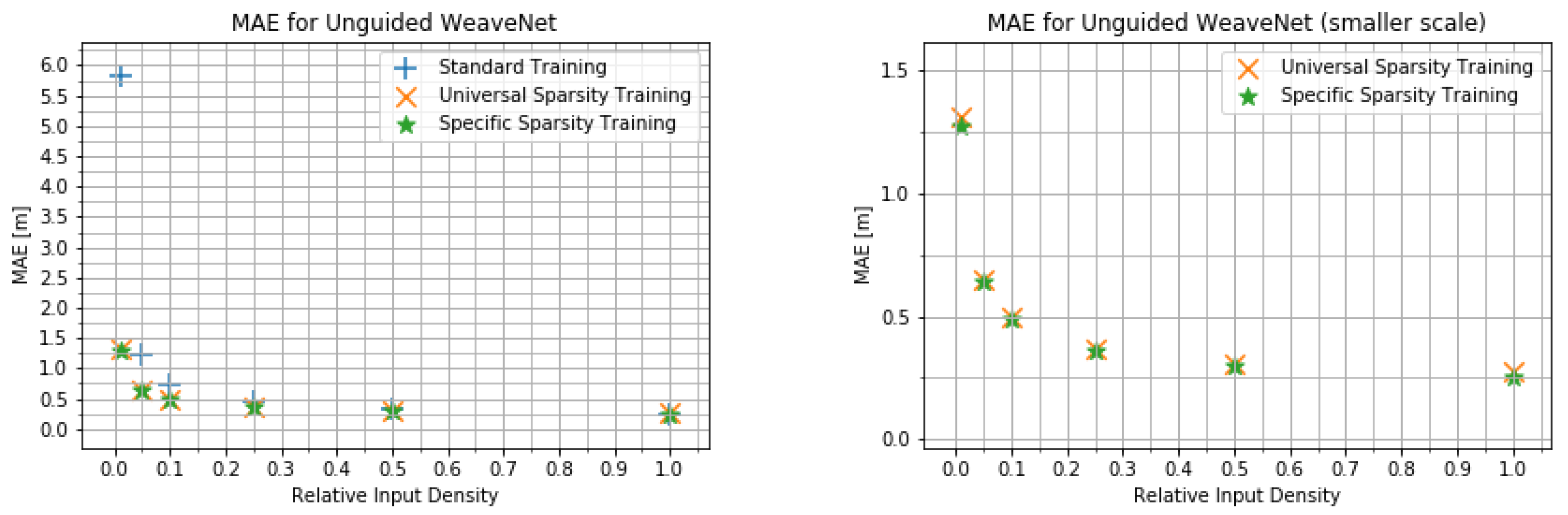
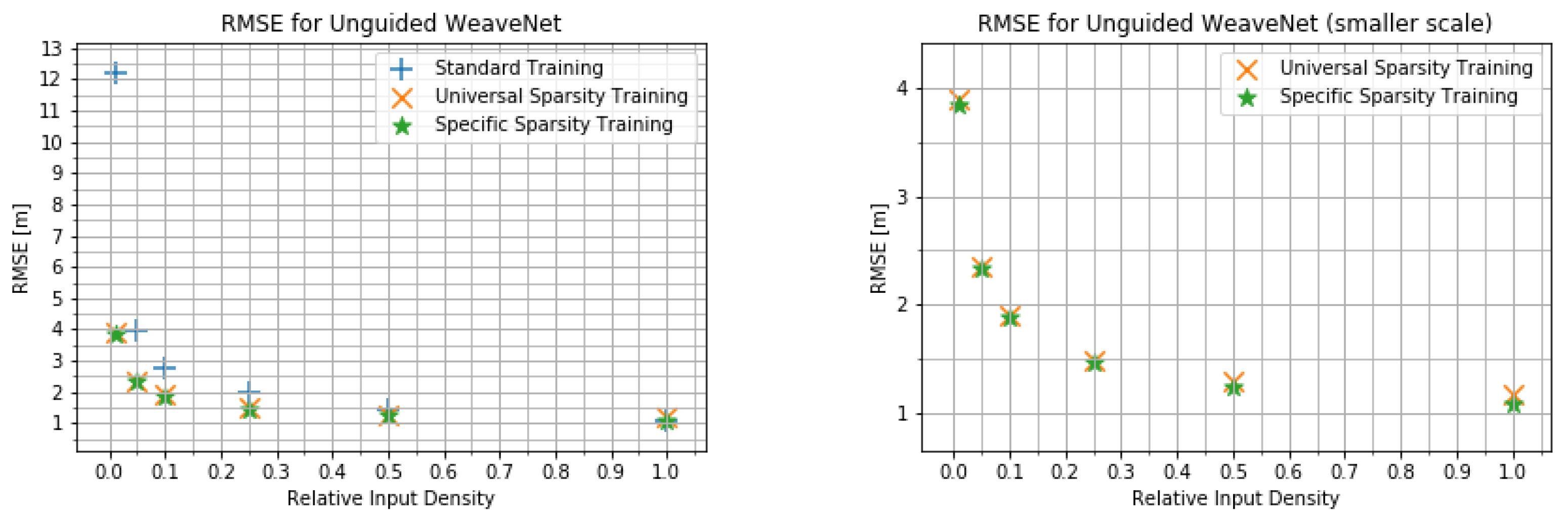
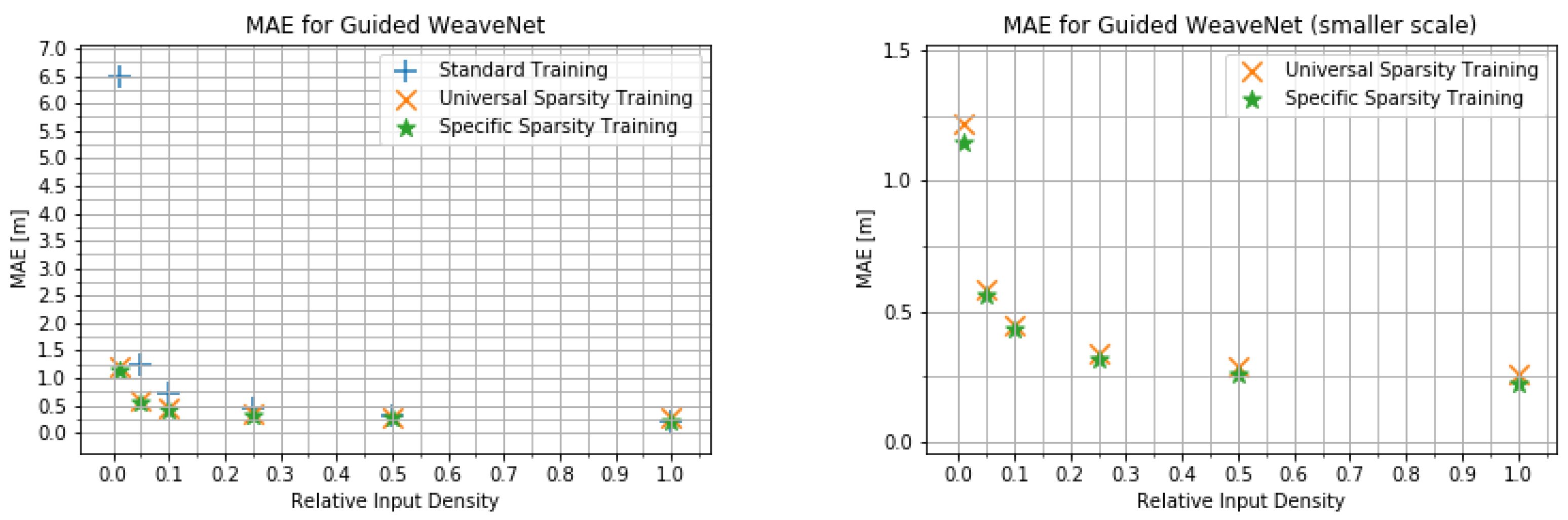
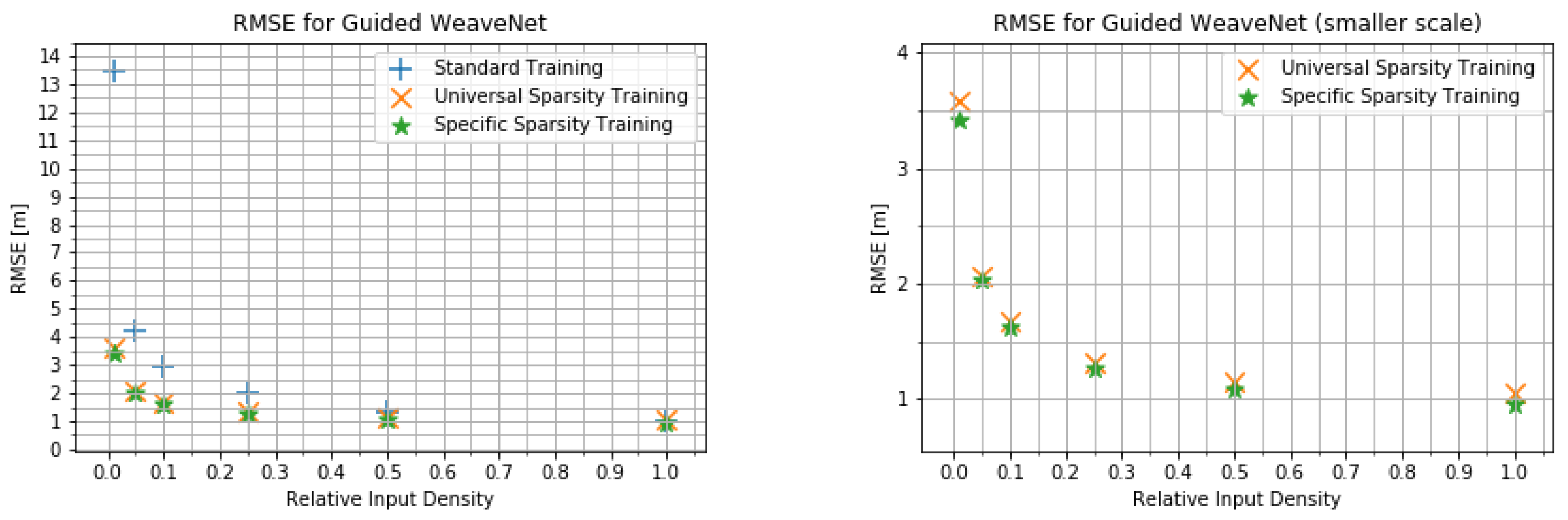
We present the quantitative results obtained using WeaveNet in Figure 4 and Figure 5 for the unguided version of the network and in Figure 6 and Figure 7 for the guided version. As can be seen in those plots, there is very little difference between the performance of the network trained for the specific input sparsity and the network trained using variable input sparsity (universal sparsity training). this points to the possibility of using the weights obtained during the universal training in systems where the number of measurements can change from one frame to another or in systems where the density of measurements may change between different parts of the FOV (such as future imaging radars).
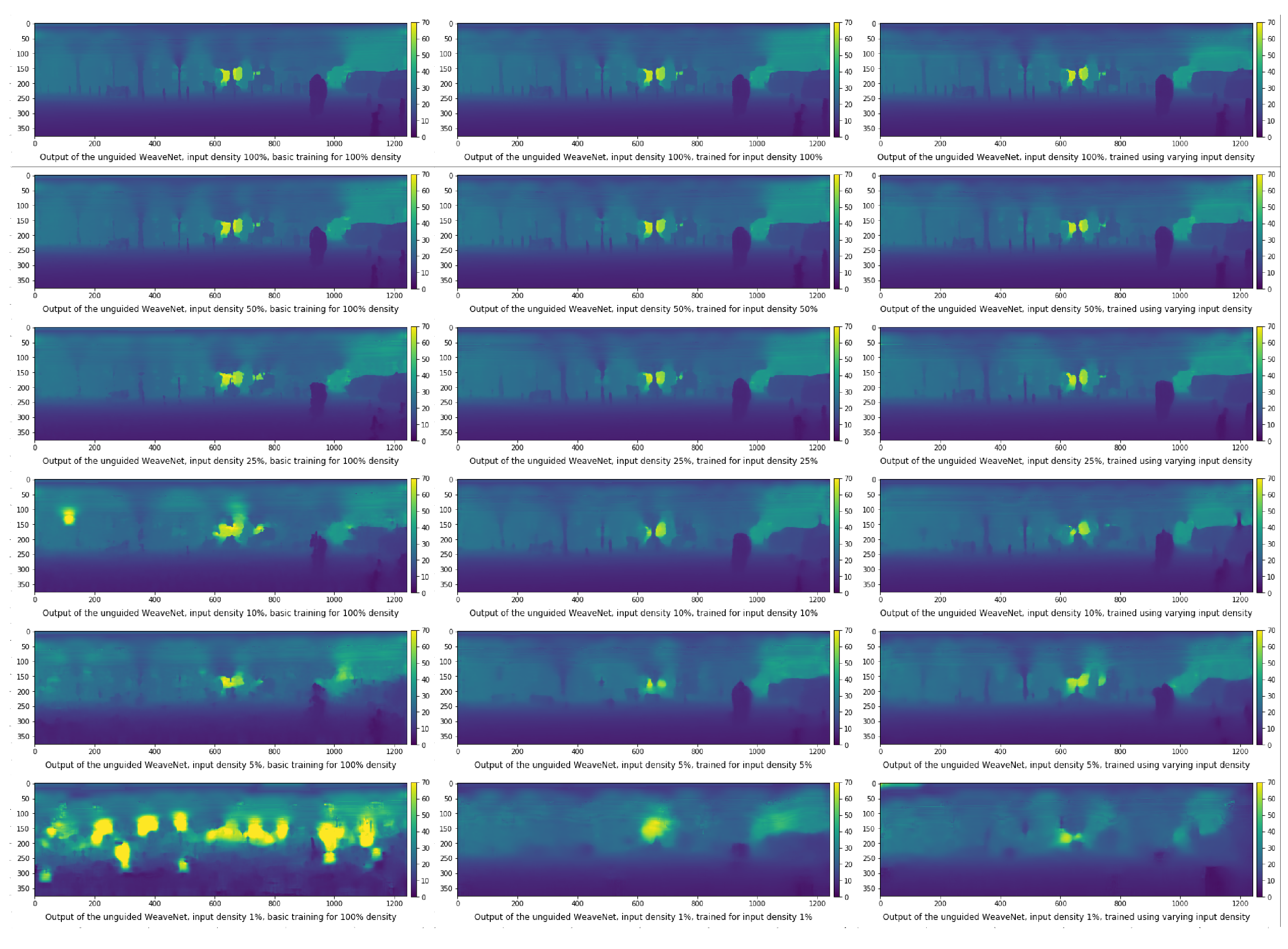
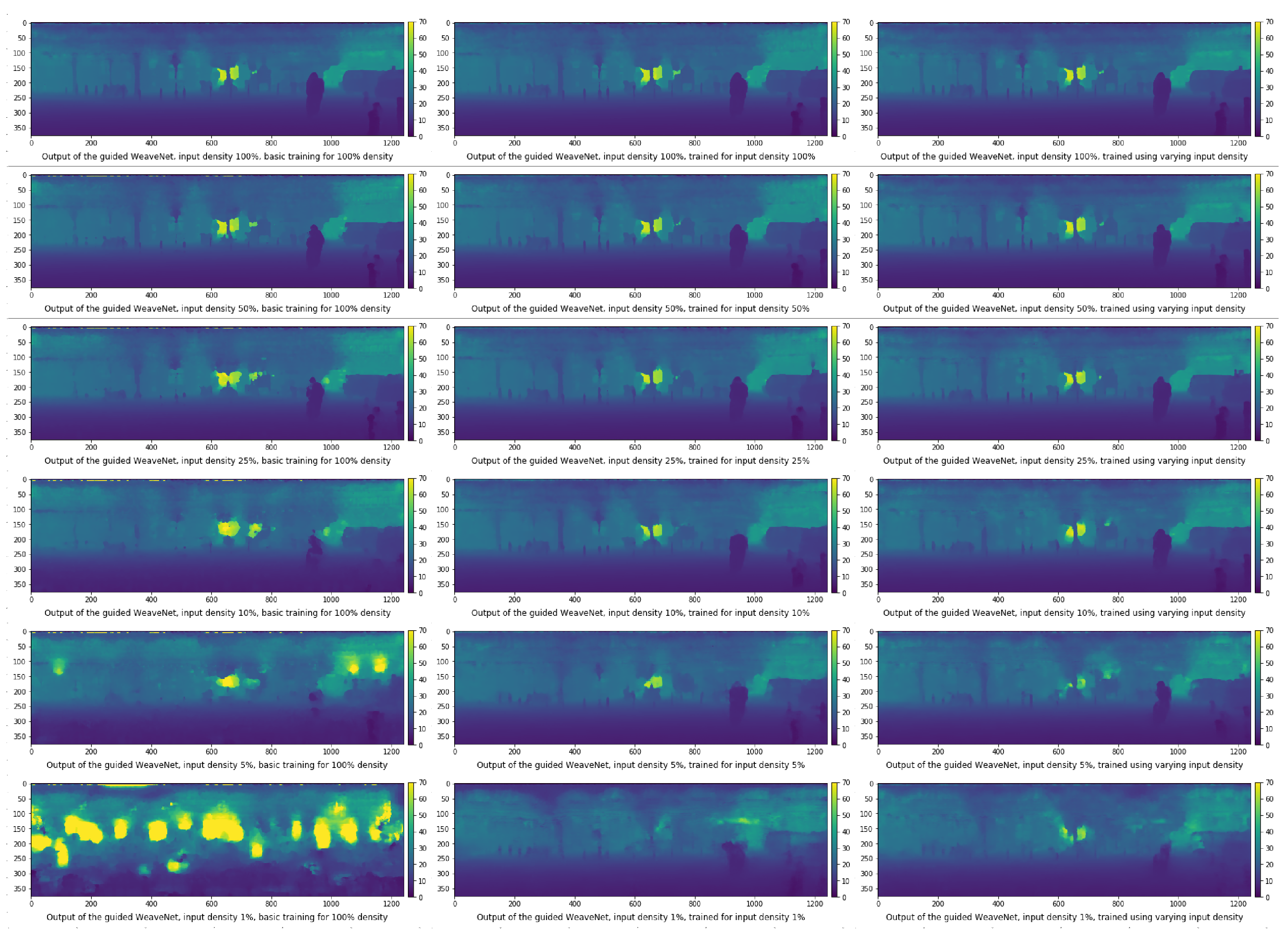
In Figure 8 and Figure 9, we show the depth output of the WeaveNet (its unguided and guided versions, respectively) for various input densities and for the three aforementioned training methods. The depth is color-coded, with the scale shown to the right of each small image. In all cases, we use the same frame as in Figure 2. Please note that there is little qualitative difference between the output produced by the version of the network trained at specific input density and the version of the network trained using variable input density (universal sparsity training). For the unguided version of the network, the fine details, such as the protection poles or street lamps, are reasonably distinguishable even at the relative input density of 10%. In the guided version, the details are still distinguishable even at 1% input density.
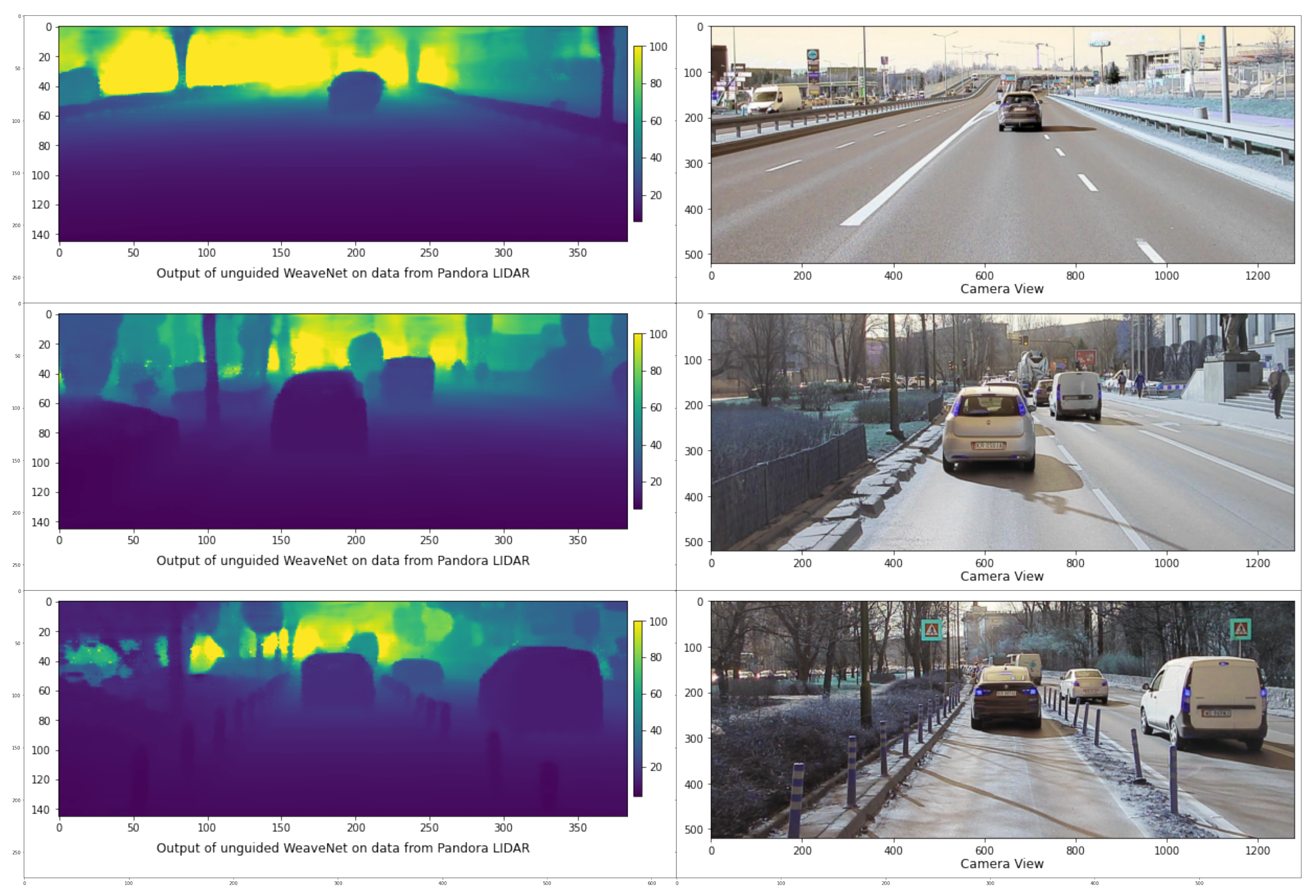
In Figure 10, we show the results of applying the unguided, universal sparsity WeaveNet to the data obtained from 40-channel Pandora LIDAR. Even though the network was trained on the KITTI dataset (using 64-channel Velodyne LIDAR), the results obtained on Pandora-sourced data look qualitatively good, which shows the robustness of the WeaveNet architecture paired with the variable input sparsity training.
5. Conclusions
In the paper, we presented a novel WeaveNet architecture capable of performing the depth completion task on very sparse input data. The results obtained by the version of the network trained using variable input sparsity are particularly promising since they point to the possibility of using depth completion methods on data from sensors producing highly variable numbers of irregularly spaced measurements. An example of such a sensor that might, in the future, benefit from depth completion is a high-resolution imaging radar. In such a radar, the amplitude of a reflected wave is highly dependent on the material and the angle of the reflection surface. Therefore, the density of reflections can vary widely between different objects in the field of view.
WeaveNet and its universal sparsity training procedure can also be useful when reusing the network weights trained on one dataset (using sensor A) to operate on the data obtained from another, depth-measuring, sensor B (as is evidenced by the qualitatively good results obtained when using the Velodyne-trained weights to perform depth completion on the Pandora-sourced data). This property can be very beneficial in settings where different sensors are tested, since it diminishes the need to create a big and expensive training set for each sensor (the model can be pretrained on the data from sensor A and later fine-tuned on a much smaller dataset using sensor B).
Another contribution of this work is the interpretation of the channels at the intermediate layers of the network. We have noted that the channels in the intermediate layers of the network either represent the interpolated depth data or are estimating the positions of object boundaries. This knowledge might help improve future depth completion networks by incorporating auxiliary losses using the intermediate layer output.
Funding
This research received no external funding.
Data Availability Statement
Not applicable.
Acknowledgments
The author is grateful to Paweł Skruch (AGH University of Science and Technology, Aptiv) and Mateusz Komorkiewicz (Aptiv) for helpful and insightful discussion.
Conflicts of Interest
The author declares no conflict of interest.
References
- Uhrig, J.; Schneider, N.; Schneider, L.; Franke, U.; Brox, T.; Geiger, A. Sparsity Invariant CNNs. In Proceedings of the International Conference on 3D Vision (3DV), Qingdao, China, 10–12 October 2017. [Google Scholar]
- Geiger, A.; Lenz, P.; Stiller, C.; Urtasun, R. Vision meets Robotics: The KITTI Dataset. Int. J. Robot. Res. 2013, 32, 1231–1237. [Google Scholar] [CrossRef] [Green Version]
- Qi, C.R.; Su, H.; Mo, K.; Guibas, L.J. PointNet: Deep Learning on Point Sets for 3D Classification and Segmentation. arXiv 2017, arXiv:1612.00593. [Google Scholar]
- Zhou, Y.; Tuzel, O. VoxelNet: End-to-End Learning for Point Cloud Based 3D Object Detection. arXiv 2017, arXiv:1711.06396. [Google Scholar]
- Huang, Z.; Fan, J.; Cheng, S.; Yi, S.; Wang, X.; Li, H. Hms-net: Hierarchical multi-scale sparsity-invariant network for sparse depth completion. IEEE Trans. Image Process. 2019, 29, 3429–3441. [Google Scholar] [CrossRef] [PubMed] [Green Version]
- Eldesokey, A.; Felsberg, M.; Khan, F.S. Propagating Confidences through CNNs for Sparse Data Regression. arXiv 2018, arXiv:1805.11913. [Google Scholar]
- Chen, Y.; Yang, B.; Liang, M.; Urtasun, R. Learning joint 2d–3d representations for depth completion. In Proceedings of the IEEE International Conference on Computer Vision, Seoul, Korea, 27 October–2 November 2019; pp. 10023–10032. [Google Scholar]
- Park, J.; Joo, K.; Hu, Z.; Liu, C.K.; Kweon, I.S. Non-Local Spatial Propagation Network for Depth Completion. arXiv 2020, arXiv:2007.10042. [Google Scholar]
- Tang, J.; Tian, F.P.; Feng, W.; Li, J.; Tan, P. Learning Guided Convolutional Network for Depth Completion. arXiv 2019, arXiv:1908.01238. [Google Scholar] [CrossRef] [PubMed]
- Qiu, J.; Cui, Z.; Zhang, Y.; Zhang, X.; Liu, S.; Zeng, B.; Pollefeys, M. DeepLiDAR: Deep Surface Normal Guided Depth Prediction for Outdoor Scene from Sparse LiDAR Data and Single Color Image. arXiv 2019, arXiv:1812.00488. [Google Scholar]
- Cheng, X.; Wang, P.; Guan, C.; Yang, R. CSPN++: Learning Context and Resource Aware Convolutional Spatial Propagation Networks for Depth Completion. arXiv 2019, arXiv:1911.05377. [Google Scholar] [CrossRef]
- Ma, F.; Cavalheiro, G.V.; Karaman, S. Self-supervised Sparse-to-Dense: Self-supervised Depth Completion from LiDAR and Monocular Camera. arXiv 2018, arXiv:1807.00275. [Google Scholar]
- Yan, L.; Liu, K.; Belyaev, E. Revisiting Sparsity Invariant Convolution: A Network for Image Guided Depth Completion. IEEE Access 2020, 8, 126323–126332. [Google Scholar] [CrossRef]
- Cheng, X.; Wang, P.; Yang, R. Learning Depth with Convolutional Spatial Propagation Network. arXiv 2019, arXiv:1810.02695. [Google Scholar] [CrossRef] [PubMed] [Green Version]
- Liu, S.; Mello, S.D.; Gu, J.; Zhong, G.; Yang, M.H.; Kautz, J. Learning Affinity via Spatial Propagation Networks. arXiv 2017, arXiv:1710.01020. [Google Scholar]
- Wang, S.; Suo, S.; Ma, W.C.; Pokrovsky, A.; Urtasun, R. Deep parametric continuous convolutional neural networks. In Proceedings of the IEEE Conference on Computer Vision and Pattern Recognition, Salt Lake City, UT, USA, 18–23 June 2018; pp. 2589–2597. [Google Scholar]
- Dosovitskiy, A.; Ros, G.; Codevilla, F.; Lopez, A.; Koltun, V. CARLA: An Open Urban Driving Simulator. In Proceedings of the 1st Annual Conference on Robot Learning, Mountain View, CA, USA, 13–15 November 2017; pp. 1–16. [Google Scholar]
- Howard, A.G.; Zhu, M.; Chen, B.; Kalenichenko, D.; Wang, W.; Weyand, T.; Andreetto, M.; Adam, H. MobileNets: Efficient Convolutional Neural Networks for Mobile Vision Applications. arXiv 2017, arXiv:1704.04861. [Google Scholar]
- Xu, B.; Wang, N.; Chen, T.; Li, M. Empirical Evaluation of Rectified Activations in Convolutional Network. arXiv 2015, arXiv:1505.00853. [Google Scholar]
- Ramachandran, P.; Zoph, B.; Le, Q.V. Searching for Activation Functions. arXiv 2017, arXiv:1710.05941. [Google Scholar]
- Clevert, D.A.; Unterthiner, T.; Hochreiter, S. Fast and Accurate Deep Network Learning by Exponential Linear Units (ELUs). arXiv 2016, arXiv:1511.07289. [Google Scholar]
- Nowak, M.K.; Lelowicz, K. Weight Perturbation as a Method for Improving Performance of Deep Neural Networks. In Proceedings of the 2021 25th International Conference on Methods and Models in Automation and Robotics (MMAR), Miedzyzdroje, Poland, 23–26 August 2021; pp. 127–132. [Google Scholar] [CrossRef]
- Kingma, D.P.; Ba, J. Adam: A Method for Stochastic Optimization. arXiv 2017, arXiv:1412.6980. [Google Scholar]
Figure 1.
Schematic representation of a residual block containing 3 WeaveBlocks.

Figure 2.
Output of the unguided WeaveNet together with the sparse LIDAR data and corresponding camera image. The edges in the output of the network are shown to demonstrate the capability of network to accurately represent fine details. The same frame is used as the basis of all future images in this paper.

Figure 3.
Example channels at the intermediate layers of WeaveNet; channels storing depth are on the left and channels storing edges are on the right).
Figure 3.
Example channels at the intermediate layers of WeaveNet; channels storing depth are on the left and channels storing edges are on the right).

Figure 4.
MAE for the unguided WeaveNet for various input densities for different training modes (different scales).
Figure 4.
MAE for the unguided WeaveNet for various input densities for different training modes (different scales).

Figure 5.
RMSE for the unguided WeaveNet for various input densities for different training modes (different scales).
Figure 5.
RMSE for the unguided WeaveNet for various input densities for different training modes (different scales).

Figure 6.
MAE for the guided WeaveNet for various input densities for different training modes (different scales).
Figure 6.
MAE for the guided WeaveNet for various input densities for different training modes (different scales).

Figure 7.
RMSE for the guided WeaveNet for various input densities for different training modes (different scales).
Figure 7.
RMSE for the guided WeaveNet for various input densities for different training modes (different scales).

Figure 8.
Output of the unguided WeaveNet for various densities for different training modes (basic training on the left, training for specific density in the middle, training for variable density on the right).
Figure 8.
Output of the unguided WeaveNet for various densities for different training modes (basic training on the left, training for specific density in the middle, training for variable density on the right).

Figure 9.
Output of the guided WeaveNet for various densities for different training modes (basic training on the left, training for specific density in the middle, training for variable density on the right).
Figure 9.
Output of the guided WeaveNet for various densities for different training modes (basic training on the left, training for specific density in the middle, training for variable density on the right).

Figure 10.
Output of the universal sparsity, unguided WeaveNet operating on the data from Pandora LIDAR (left) and corresponding camera images (right).
Figure 10.
Output of the universal sparsity, unguided WeaveNet operating on the data from Pandora LIDAR (left) and corresponding camera images (right).


Table 1.
Performance of the RGB-guided depth completion methods on the KITTI validation set.
| Model | RMSE [m] | MAE [m] |
|---|---|---|
| Eldesokey et al. [6] | 1.37 | 0.38 |
| Tang et al. [9] | 0.77778 | 0.22159 |
| Park et al. [8] | 0.88410 | not provided |
| Cheng et al. [11] | 0.72543 | 0.20788 |
| Chen et al. [7] | 0.75288 | 0.22119 |
| Qiu et al. [10] | 0.68700 | 0.21538 |
| Yan et al. [13] | 0.79280 | 0.22581 |
| Ma et al. [12] | 0.856754 | not provided |
| Huang et al. [5] | 0.88374 | 0.25711 |
| Ours (standard training) | 0.97175 | 0.22060 |
| Ours (universal sparsity training) | 1.05978 | 0.26249 |
| Ours (specific sparsity training) | 0.94849 | 0.22623 |
Table 2.
Performance of the unguided depth completion methods on the KITTI validation set.
| Model | RMSE [m] | MAE [m] |
|---|---|---|
| Uhrig et al. [1] | 2.01 | 0.68 |
| Ma et al. [12] | 0.99135 | not provided |
| Huang et al. [5] | 0.99414 | 0.26241 |
| Ours (standard training) | 1.09596 | 0.24512 |
| Ours universal sparsity training) | 1.17372 | 0.27323 |
| Ours (specific sparsity training) | 1.08774 | 0.25310 |
Publisher’s Note: MDPI stays neutral with regard to jurisdictional claims in published maps and institutional affiliations. |
© 2022 by the author. Licensee MDPI, Basel, Switzerland. This article is an open access article distributed under the terms and conditions of the Creative Commons Attribution (CC BY) license (https://creativecommons.org/licenses/by/4.0/).
Share and Cite
MDPI and ACS Style
Nowak, M.K. WeaveNet: Solution for Variable Input Sparsity Depth Completion. Electronics 2022, 11, 2222. https://doi.org/10.3390/electronics11142222
AMA Style
Nowak MK. WeaveNet: Solution for Variable Input Sparsity Depth Completion. Electronics. 2022; 11(14):2222. https://doi.org/10.3390/electronics11142222
Chicago/Turabian StyleNowak, Mariusz Karol. 2022. "WeaveNet: Solution for Variable Input Sparsity Depth Completion" Electronics 11, no. 14: 2222. https://doi.org/10.3390/electronics11142222
Note that from the first issue of 2016, this journal uses article numbers instead of page numbers. See further details here.