Signals Recognition by CNN Based on Attention Mechanism

Abstract

Automatic modulation recognition is a key technology in non-collaborative communication. However, it is affected by complex electromagnetic environments, leading to low recognition accuracy. To address this problem, this paper develops a ResNext signal recognition model based on an attention mechanism. Firstly, a channel, including additive Gaussian white noise (AWGN), Rician multipath fading, and clock offset, is created to simulate the complex electromagnetic environment, and transmission-impaired modulated signals with various signal-to-noise ratios (SNRs) are synthesized as a dataset. Secondly, using parallel stacked residual blocks of the same topology, instead of the residual blocks of ResNet, and introducing the attention layer (CBAM), the types of feature extraction are enriched without significantly increasing the parameter order of magnitude and avoiding the over-fitting phenomenon caused by depth deepening. The results show that the signal recognition method, based on the improved neural network framework, outperformed other deep learning methods, and the recognition rate obtained of 10 different modulation types of signals was above 90% at SNRs greater than 0 dB. The proposed signal recognition method achieved accurate recognition in complex electromagnetic environments.

1. Introduction

Automatic modulation recognition (AMR) is a pivotal technique of non-collaborative communication, which refers to automatically recognizing the modulation type of the signal by the receiver with limited or no prior information, providing the basis for subsequent signal extraction and processing [1,2]. With the development of software-defined radio technology and the increasingly complex electromagnetic environment, the wireless channels of various kinds of noise and interference are gradually increasing. Traditional modulation recognition technology for communication signals has been unable to effectively carry out recognition, which represents a severe test for modulation recognition technology. Therefore, how to efficiently and accurately realize the modulation recognition of communication signals has attracted more and more attention. Typical modulation recognition techniques can broadly be divided into three categories: likelihood ratio recognition methods based on decision theory (LB), pattern recognition methods based on feature extraction (FB), and deep learning recognition methods [3,4].

LB methods [5,6,7,8,9] make decisions by calculating the likelihood function of the received signals and then comparing it to a certain threshold. Although LB methods can minimize the error rate, their high computational complexity make them unsuitable for applications such as unknown channels and clock offsets due to inaccurate internal clock sources between the transmitter and the receiver [2]. FB methods [10,11,12,13] require the manual calculation of certain features of the received signal, such as the normalized central amplitude mean, standard deviation and kurtosis, normalized absolute instantaneous frequency, higher-order moments, higher-order volume accumulation, cyclic moments, and other features. Although the computational complexity of these features is relatively low, the characteristics are overly dependent on manual analysis for their selection. It is difficult to characterize multiple modulation types in complex electromagnetic environments. Therefore, AMR is a very challenging task, especially when there is no prior information about the received signal in non-collaborative communication [1].

In recent years, due to the development of neural network units, such as hidden layers and non-linear activation, deep neural networks have been particularly prominent in image classification, machine translation, and natural language processing [14,15,16,17,18,19,20], as deep learning models can extract deeper information hidden in the data. At present, deep learning is also progressively being applied to wireless communication and radio signal processing. In modulation recognition, deep learning methods obtain better performance than FB methods. For instance, ref. [21] used a convolutional neural network (CNN) for modulation recognition, which was shown experimentally to be close to the FB method and had greater flexibility in detecting various modulation types. To further improve performance, ref. [22] introduced a densely connected network (DenseNet) to deepen the feature propagation in deep neural networks by creating shortcut paths between different layers of the network. A convolutional long short-term deep neural network (CLDNN) was introduced in [23], which exploits the complementary nature of CNN and LSTM to combine the architectures of CNN and long short-term memory (LSTM) into deep neural networks. The main difference between the deep learning-based modulation recognition system and the traditional modulation recognition system is that the feature extraction is automatically learned by the neural network, which avoids the feature design process and is more appropriate for application in non-collaborative communication scenario requirements.

Existing methods are often inaccurate in estimating the reality of complex electromagnetic environments and signal-to-noise ratios (SNRs). Realistic channel SNRs may be unstable or rapidly changing under certain circumstances. Although the use of simulated and synthetic data sets for learning is not favored in deep learning, the field of radio communication is a special case. As the real complex electronics environment is quantified as much as possible, and as simulation methods are refined, the gap between synthetic and real data sets will narrow. This will facilitate modulation identification in complex electromagnetic environments. This paper simulates a complex electromagnetic environment by constructing channels containing additive white Gaussian noise (AWGN), Rician multipath fading, and clock offset. Modulated signals with 10 kinds of transmission impairments under different SNRs are synthesized into a dataset. A network model based on ResNext is then established, the residual blocks in the traditional ResNet are replaced with a residual block of the same topology stacked in parallel and an attention layer CBAM is introduced, connected behind each convolution block of ResNext. The impaired I/Q signals are used directly as input, by increasing the dimension of ‘cardinality’ to extract greater signal features and improve the accuracy of modulation recognition. Simulation results show that the established network outperforms other neural networks.

The remainder of this paper is organized as follows. Section 2 describes the construction of the signal recognition model. Section 3 discusses the experimental results. Section 4 provides the conclusions.

2. System Models and Scenatios

AMR is an intermediate process that occurs between signal detection and receiver demodulation. Compared with the traditional method, the structure of the proposed AMR method in this paper is shown in Figure 1. The preprocessing in Figure 1 refers to the sampling and quantization of the IF signal. The traditional AMR process, as shown in the dashed box, contains the extraction, selection, and classifier of expert features, which is replaced by the CNN method in this paper. Moreover, provided that the SNR range of the communication channel is known, CNN can learn the characteristics adapted to the corresponding conditions. This property means that the method proposed is unrelated to SNR estimation.

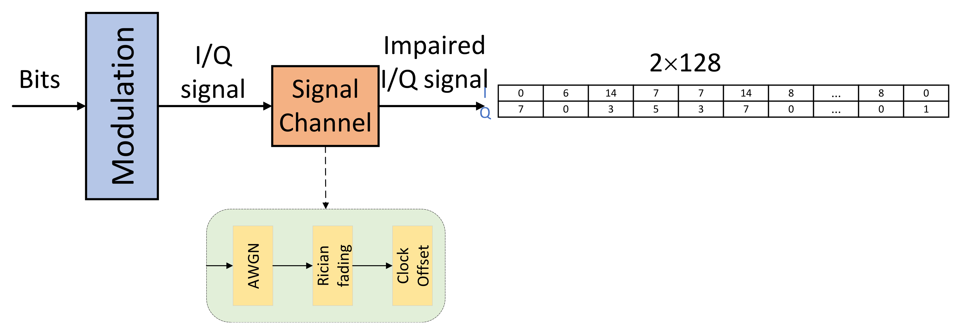
2.1. Signal Model

Modulation recognition can be expressed as a classification problem with N modulations. This paper focuses on the modulated signal affected by the complex electromagnetic environment; the received signal $r\left(t\right)$ is described in Equation (1):

$$r\left(t\right)=s\left(t\right)+g\left(t\right)$$

(1)

where $g\left(t\right)$ is the additive white Gaussian noise (AWGN), $s\left(t\right)$ is the transmit signals of different modulation types, and SNR is defined as $P_s/P_n$ ($P_s$ is the signal power, $P_n$ is the noise power). The commonly used modulation methods are as follows:

When the transmit signal is a PSK or FSK signal, $s\left(t\right)$ can be expressed in Equation (2) as follows:

$$s\left(t\right)=\left[A_m{\displaystyle \sum _n}{a}_{n}n(t-n{T}_s)\right]cos(2\pi (f_c+f_m)t+{\mathsf{\Psi }}_0+{\mathsf{\Psi }}_m)$$

(2)

where $A_m$ and $a_n$ are the modulation amplitude and symbol sequence, respectively, $n\left(t\right)$ is the signal pulse, and $T_s$ denotes the symbol period. $f_c$ and $f_m$ denote the carrier frequency and modulation frequency. ${\mathsf{\Psi }}_0$ and ${\mathsf{\Psi }}_m$ denote the initial phase and modulation phase, respectively.

When the transmit signals are M-QAM signals, which is slightly different from PSK and FSK signals in that there are two quadrature carriers and the two carriers are modulated by $a_n$ and $b_n$, respectively, $s\left(t\right)$ can be expressed in Equation (3):

$$\begin{array}{c}\hfill s\left(t\right)=\left[A_m{\displaystyle \sum _n}{a}_{n}n(t-n{T}_s)\right]cos(2\pi f_{c}t+{\mathsf{\Psi }}_0)\\ \hfill +\left[A_m{\displaystyle \sum _n}{b}_{n}n(t-n{T}_s)\right]sin(2\pi f_{c}t+{\mathsf{\Psi }}_0)\end{array}$$

(3)

After determining the transmitting signal $s\left(t\right)$, for the actual radio wave propagation channel, the electromagnetic waves will be transmitted from different paths to the receiver through reflections from multiple objects, creating a multipath effect. However, since there are different transmission paths with different time delays, each propagation path will change with time, and the interrelationship between the component fields involved in the interference will also change with time, causing random changes in the synthetic wave-field, and thus causing the fading of the total received field. In a multipath propagation scenario with a strong path, the received signal is a statistical model of a multipath channel whose impulse response amplitude follows Rician fading $\alpha \left(t\right)$.

A clock offset is caused by inaccurate internal time sources of the transmitter and receiver. Clock offset causes the center frequency (used to down-convert the signal to baseband) and the digital-to-analog converter (DAC) sample rate to be different from the ideal value. Therefore, it is necessary to perform frequency offset $f_0$ and phase offset ${\theta }_0$ on the signal based on the clock offset factor and the center frequency.

To simulate the complex electromagnetic environment, it is necessary to add Rician multipath fading, frequency offset, and phase offset to the channel. The received sampled signal $r\left(t\right)$ can be re-expressed in Equation (4).

$$r\left(t\right)=\alpha \left(t\right)e^{j(2\pi f_{0}t+{\theta }_0\left(t\right))}s\left(t\right)+g\left(t\right)$$

(4)

The purpose of modulation recognition is to determine the $P(s\left(t\right)\in N\left(i\right)\left|r\left(t\right)\right.)$ after receiving the signal $r\left(t\right)$, where $N\left(i\right)$ denotes the i-th modulation, and the goal is to recognize the modulation type i from the received signal $r\left(t\right)$. For simplicity, the received signal is usually represented by its in-phase and quadrature $I/Q$ components, which represent the $r\left(t\right)$ real and imaginary parts, respectively. For this purpose, the ResNext network, based on the attention mechanism, is used to learn recognition, first processing the dataset to set the network parameters and then calculating the recognition accuracy on the test dataset.

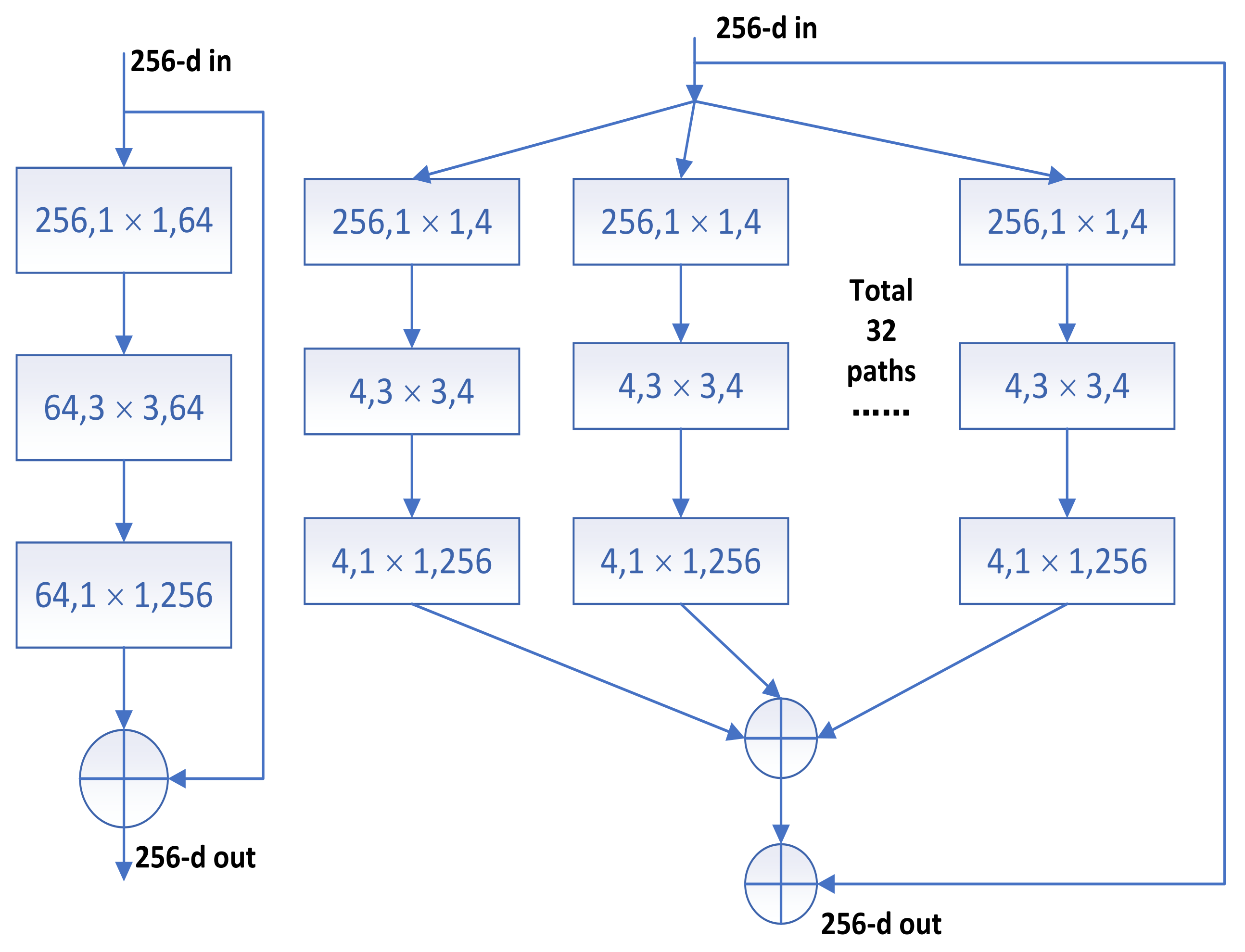
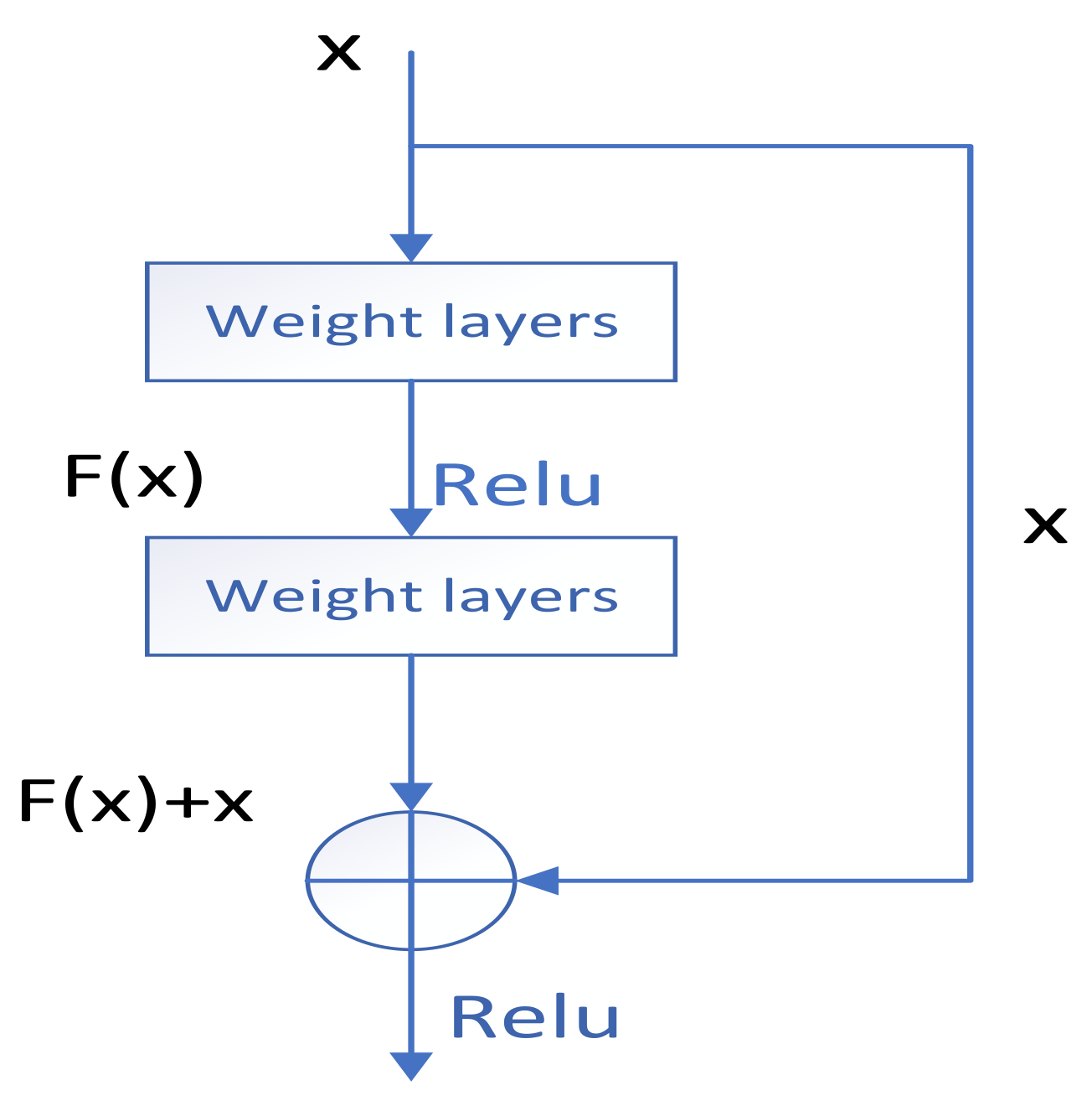
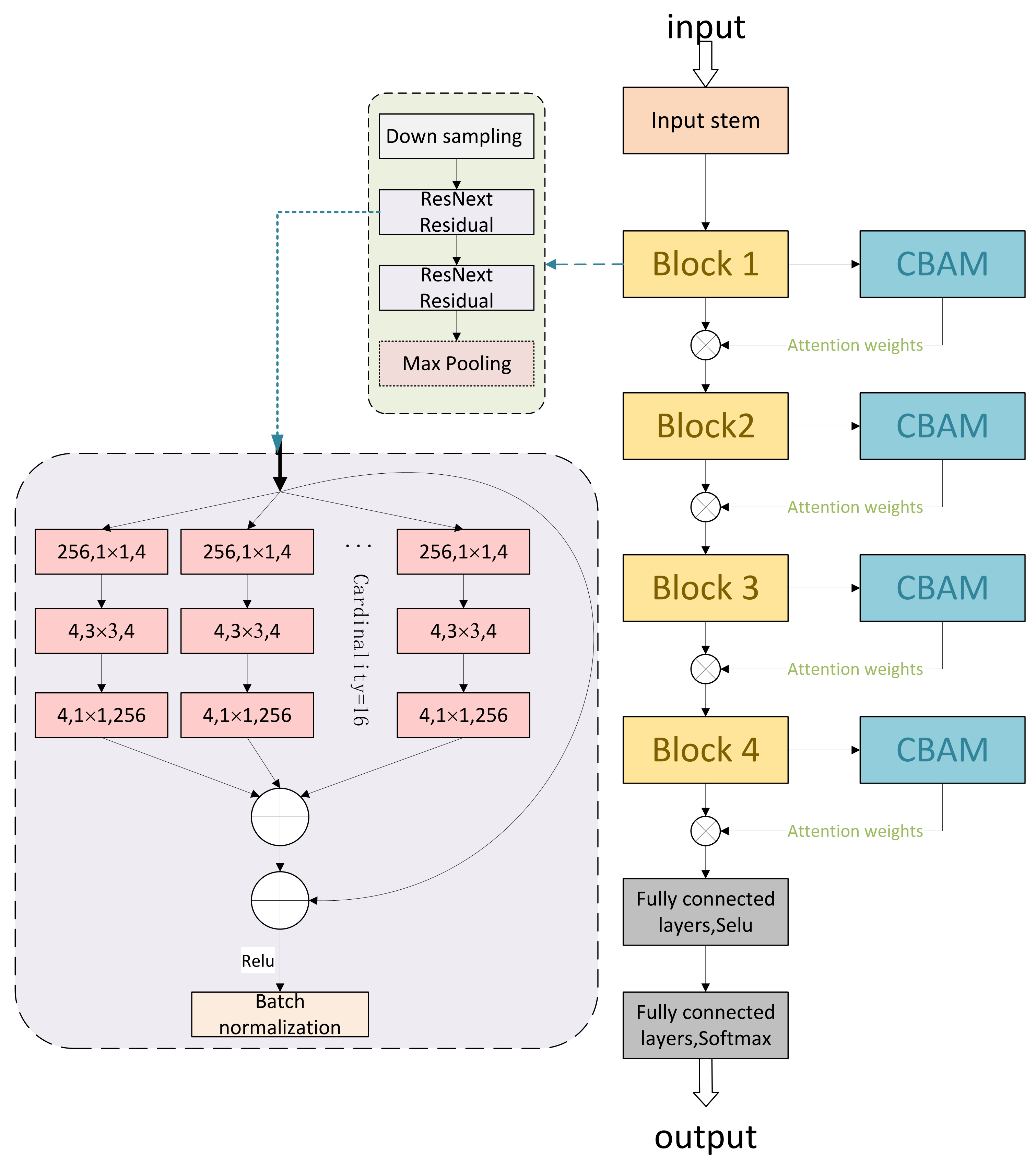
2.2. Network Model

Theoretically, the more layers of a deep learning model network there are, the better the performance should be. In practice, as the number of network layers increases, the gradient disappears and the gradient explodes, resulting in poor recognition performance. However, due to the topology of the sub-modules, the ResNext structure can improve accuracy without increasing parameter complexity, while also reducing the number of hyper-parameters. As shown in Figure 2, with parallel stacking of blocks of the same topology, instead of the three-layer convolution block of the original ResNet, the accuracy of the model is improved without significantly increasing the parameter order. At the same time, due to the same topology, the hyper-parameters are also reduced, which is convenient for model porting.

To further improve the performance of the ResNext network model and select the most discriminative features, an attention mechanism is introduced into the ResNext network model to explore the dependencies between features. The attention mechanism is a common data processing method in deep learning and is widely used in various deep learning tasks, such as natural language processing, image recognition, and speech recognition. Assembling features by assigning larger weights to some ‘significant’ features not only reduces the parameters of the network but also improves the discriminative power of the features.

A convolutional block attention module (CBAM) is an attention module that can be inserted into convolutional neural networks. A CBAM will infer the attention map along two independent dimensions (channel and spatial) accordingly, and then multiply the attention map with the input feature map to perform adaptive feature optimization. As shown in Figure 3, the output result of the convolution layer is first weighted by the channel attention module, and then passed through the spatial attention module to obtain the final result.

The channel attention module, as shown in Figure 4a, compresses the feature map in the spatial dimension and then operates after obtaining a one-dimensional vector. The input feature maps are compressed by the MaxPooling layer and the MeanPooling layer, and then sent to the shared fully connected layer. Then the results of the shared fully connected layer are summed and activated by the activation function sigmoid to obtain the final channel attention weights $M_C\left(F\right)$, which can be expressed in Equation (5).

$$M_C\left(F\right)=\sigma \left(W_1\right(W_0\left(F_{avg}^c\right))+\left(W_1\left(W_0\left(F_{max}^c\right)\right)\right)$$

(5)

where F is the input feature mapping, and $W_0$ and $W_1$ represent the weight matrices of the hidden layer and the fully connected layer, respectively.

The spatial attention module in Figure 4b can be regarded as channel compression, performing MeanPooling and MaxPooling on the feature maps of the channel dimension. The previously obtained feature maps (the number of channels is equal to 1) are merged to obtain a two-channel feature map, and to obtain the spatial attention weight $M_s\left(F\right)$, which can be expressed in Equation (6).

$$M_S\left(F\right)=\sigma \left(f^{7\times 7}\left([F_{avg}^s;F_{max}^s]\right)\right)$$

(6)

where $\sigma$ is the sigmoid activation operation and $f^{7\times 7}$ represents the kernel size of the convolution.

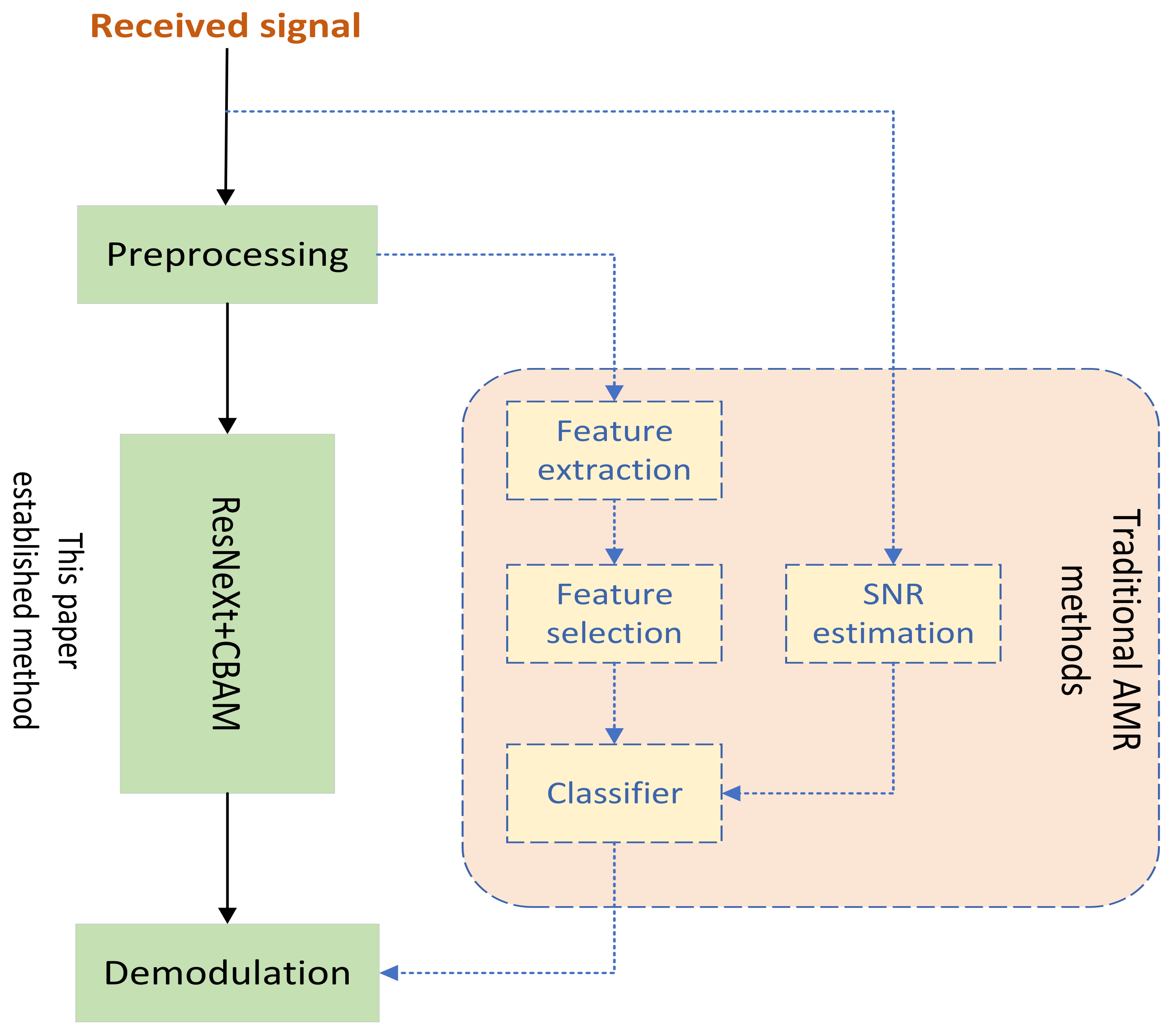
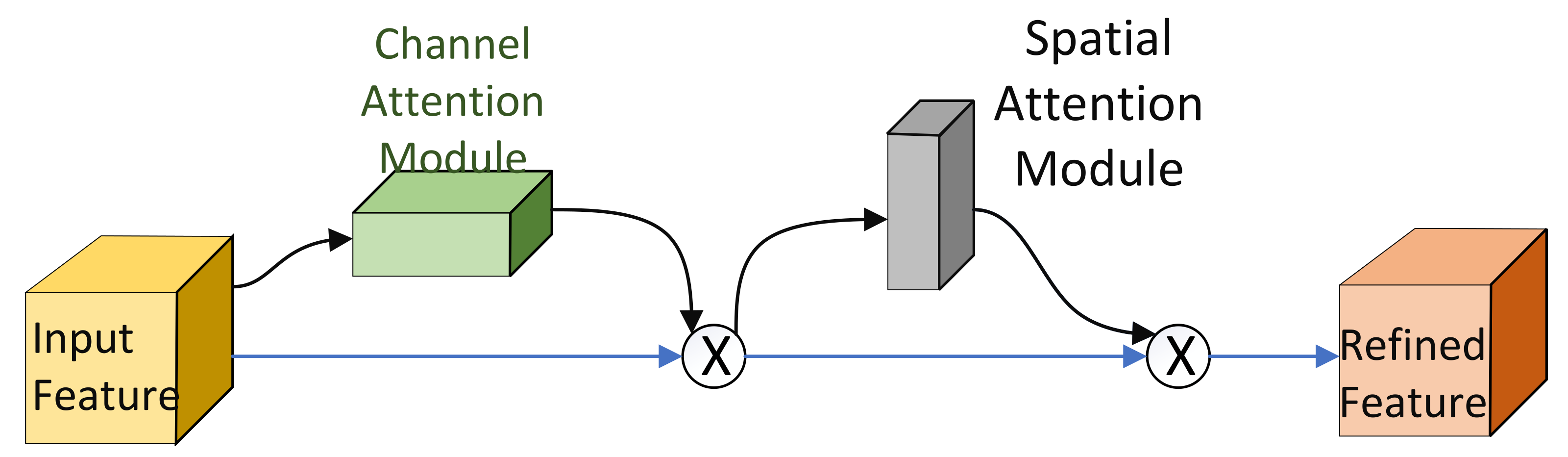
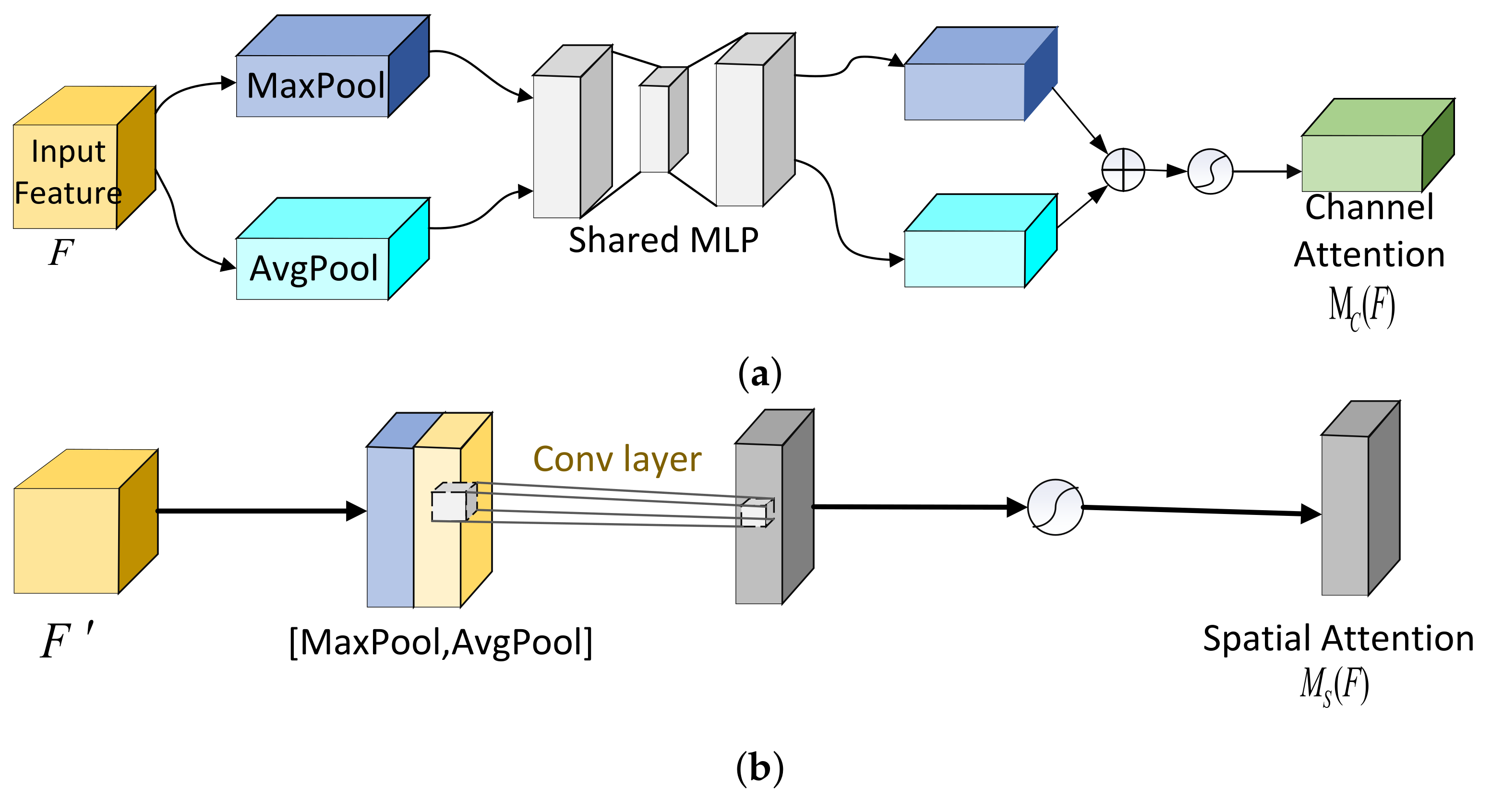
2.3. CNN Signal Recognition Model Based on Attention Mechanism

The ResNext network introduces residual connections between convolutional blocks and adds the output to the input of the convolutional blocks to optimize the training process, overcoming the degradation problem of deep neural networks, and achieving better recognition. The basic structure of the residual unit is shown in Figure 5, where x represents the input of the first layer and the expectation output function is $H\left(x\right)$, i.e., $H\left(x\right)$ is the expected complex potential mapping; however, such a model would be very difficult to train. Therefore, the learning objective is transformed into the learning of the identity map; that is, the input x is approximated to the output $H\left(x\right)$ to keep the accuracy in the later layers without loss. Through shortcut connection, the input x is passed directly to the output as the initial result, and the output is $H\left(x\right)=F\left(x\right)+x$. When $F\left(x\right)=0$, then $H\left(x\right)=x$, which is the identity mapping. Thus, the learning objective shifts from the original learning complete output to the difference between the learning target value $H\left(x\right)$ and x, which is the residual function $F\left(x\right)=H\left(x\right)-x$. Therefore, the training objective is to approximate the residual function to 0 such that the accuracy does not decrease as the network deepens.

Figure 6 shows the network structure designed for automatic feature extraction of 10 types of modulated signals. Based on ResNext, the CBAM module is introduced and connected after each convolutional block of ResNext. It consists of four convolutional modules and two fully connected layers, where each convolutional block consists of a down-sampling layer and two ResNext residual blocks, and a MaxPooling layer. In each ResNext residual block, to avoid the gradient disappearance and slow network convergence caused by the internal covariate shift during the training process, it is necessary to batch normalize the activation values at the end. The original radio signal first enters the convolution module through the input layer, and the convolution module inputs the extracted features to the attention layer, weights the features in the attention layer, and finally inputs to the next layer after the cascade processing of nodes. The final features are fed to fully connected layers for subsequent classification. The first fully connected layer uses the Selu scaling exponential linear unit activation function, and the second fully connected layer uses the Softmax activation function with an output size of 10.

During the network training process, the cross-entropy loss function in Equation (7) is chosen to evaluate the network.

$$Loss=-\frac{1}{N}\sum _{i=1}^{N}log\left(oM\right(i\left)\right)$$

(7)

where N represents the number of training samples and $oM\left(i\right)$ represents the prediction probability that the i-th sample belongs to class $M\left(i\right)$. The training process uses Adam optimizer back-propagation to update all network parameters (including convolutional, attention and fully connected layers).

3. Experiment and Analysis

3.1. Dataset

The realistically complex electromagnetic environment has many effects on the transmitted signals, which makes it very difficult to simulate. Although the use of simulated and synthetic data sets for learning is not favored in deep learning, the field of radio communication is a special case. Automatic modulation recognition models require large amounts of labeled data for training, and, with a complex electromagnetic environment, this makes it difficult to capture and label radio signals. As the realistically complex electromagnetic environment is quantified as much as possible, introducing unknown scales, translations, inflation and noise into our models, the gap between synthetic and real datasets will narrow as the simulation methods become better. The use of simulated and synthetic datasets will become an increasingly important tool when real data is difficult to capture or label.

The establishment of the dataset is shown in Figure 7. Bits are modulated and passed through the channel, including AWGN, Rician fading and clock offset, to synthesize 10 types of transmission-impaired IQ signals under various SNRs.To generate well-characterized data sets, ten widely used modulations are selected: eight digital modulations and two analog modulations. These include 8-PSK, BPSK, CPFSK, GFSK, 4-PAM, 16-QAM, 64-QAM, QPSK for digital modulation, and WB-FM and AM-DSB for analog modulation.

The dataset parameters are also set as close as possible to the realistically complex electromagnetic environment. The sampling frequency $f_s$ affects the classification performance only in the fading channel, and the Rician channel is modeled as a flat channel when $f_s$ = 200 kHz. In the flat channel, the multipath structure of the channel allows the spectral characteristics of the transmitted signal to be preserved on the receiver side. Taking into account that the length of the signal sequence may have an impact on the results, the model shown in Figure 6 is used to train on datasets with sequence lengths of 32, 128, and 256, respectively. The over-sampling rate is 4. Other signal parameters are set as follows: the SNR range is [−6, 4], and the step size is 2 dB. The center frequencies of digital and analog modulation types are 902 MHz and 100 MHz, respectively. A total of 10,000 data points are generated for each modulation type at each SNR, of which 80% are used for training, 10% for validation, and 10% for testing. Figure 8 shows the effect of different sequence lengths on the recognition results, so the dataset with sequence length L = 128 was chosen as the input to the modulation recognition model.

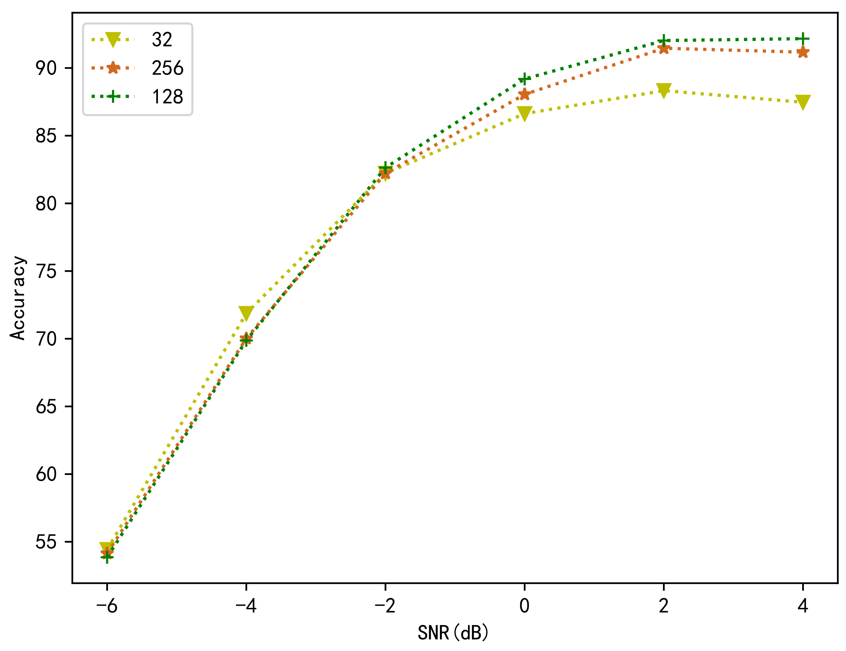
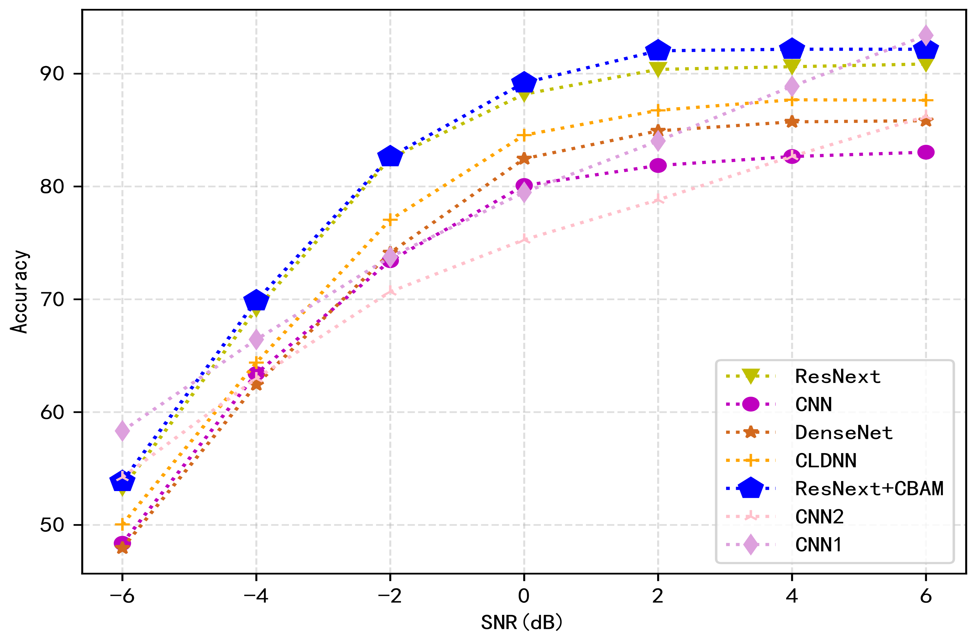
3.2. Performance Comparison Analysis

To demonstrate the advantages of the model established in this paper, seven different models of CNN [21], DenseNet [22], CLDNN [23], CNN1 [24], CNN2 [24] and ResNext were trained using the same training set. Then the best model and the parameters after training were saved, and the test set was used to obtain the recognition accuracy under different SNRs.

From the comparative performance plots of various neural networks given in Figure 9, it is clear that the recognition accuracy of all five networks increased with increase in SNR due to there being less noise at high SNR. Under high SNR, ResNext + CBAM and ResNext were able to achieve more than 90% recognition accuracy, which was the best result among all models, due to the residual connection method and the topology of ResNext’s group convolution. The ResNext model, with introduction of a CBAM attention layer, was about 3% higher than the ordinary ResNext model, reflecting the benefit of introducing a CBAM attention mechanism, which can help to extract effective features from noise-contaminated data.

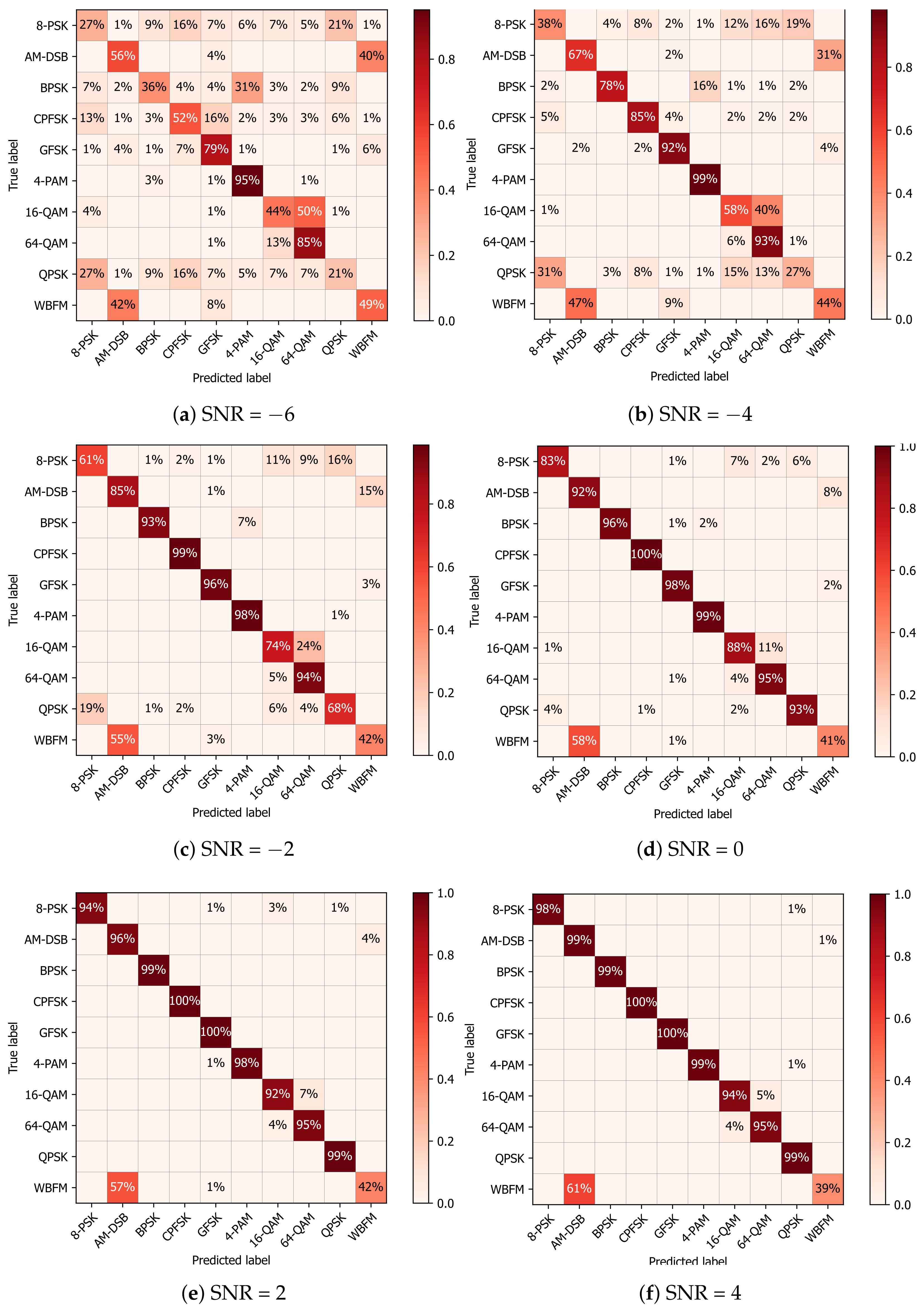
3.3. Analysis of Results

The training set was used to train the network shown in Figure 6, using the overall accuracy (OA) to evaluate the recognition results of the built model. A total of 40 independent experiments were conducted to complete the recognition of 10 types of modulated signals with impaired transmission; the average OA of the classification results was 80.57%. For further confirmation, the recognition results of the test set under several SNRs were selected and presented in the form of confusion matrices.

The network parameters of this design are set as follows: the cross-entropy loss function is used to view the change in the loss value during the training process, and the optimizer selects Adam, where the learning rate is 0.001. The learning rate becomes 0 after each parameter update, and the updated exponential decay rate is ${\beta }_1=0.9$, ${\beta }_2=0.999$. The batch_size = 512 in the training process; after each iteration, the training data is re-shuffled. When the training loss value is reached for 10 consecutive iterations without reducing, the training is stopped, the trained model saved and the weight parameters are used in testing.

The variation in the training accuracy function (dashed line) and the validation accuracy function with the number of iterations is shown in Figure 10. It can be seen that as the number of training iterations increases, the values of both the training accuracy function and the validation accuracy function increase and finally reach a stable value at 40 iterations.

The confusion matrix tested at SNRs ranging from −6 dB to 4 dB with a step size of 2 dB is shown in Figure 11; the numbers in the percentage column indicate the percentage of the left signal type that were a misrecognition of the right signal type. Figure 11a shows that SNR = −6 dB and OA = 54.86%. Figure 11b shows that SNR = −4 dB and OA = 69.87%. Figure 11c shows that SNR = −2 dB and OA = 82.95%. Figure 11d shows that SNR = 0 dB and OA = 89.19%. Figure 11e shows that SNR = 2 dB and OA = 92.78%. Figure 11f shows that SNR = 4 dB and OA = 92.17%. It can be seen that the established model can accurately identify most signal types, while for AM-DSB and WBFM, 16-QAM and 64-QAM have poor recognition results. This is because, when the data set is generated, the observation window is small, the information rate is low, and the correlation between the information is small, so it is difficult to distinguish AM-DSB and WBFM. For 16-QAM and 64-QAM, due to the amplitude characteristics and phase information of the QAM signal, the I/Q signals of these two signals are similar, and it is difficult to classify and recognize them.

4. Conclusions

Due to the complexity of the wireless communication environment, it is difficult to obtain high recognition accuracy in practical applications. In this paper, an attention-mechanism-based ResNext model is established, and Matlab simulation is used to generate a modulated signal with impaired transmission in a complex electromagnetic environment as the dataset. The final results show that more than 90% recognition accuracy was able to be achieved when the SNR is greater than 0 dB.

The established network model outperforms the CNN, DenseNet, CLDNN, and ordinary ResNext models. By introducing an attention mechanism, the recognition accuracy is improved by about 3%, which enriches the types of signal feature extraction and avoids the occurrence of overfitting and gradient disappearance phenomena. High accuracy is achieved for modulation recognition in complex electromagnetic environments.

References

- Zhu, Z.; Nandi, A.K. Automatic Modulation Classification (Principles, Algorithms and Applications); John Wiley & Sons: Hoboken, NJ, USA, 2014. [Google Scholar] [CrossRef]
- Dobre, O.A.; Abdi, A.; Bar-Ness, Y.; Su, W. Survey of automatic modulation classification techniques: Classical approaches and new trends. IET Commun. 2007, 1, 137–156. [Google Scholar] [CrossRef] [Green Version]
- Huang, S.; Yao, Y.; Wei, Z.; Zhang, P. Automatic Modulation Classification of Overlapped Sources Using Multiple Cumulants. IEEE Trans. Veh. Technol. 2017, 66, 6089–6101. [Google Scholar] [CrossRef]
- Tian, J.; Pei, Y.; Huang, Y.D.; Liang, Y.C. Modulation-Constrained Clustering Approach to Blind Modulation Classification for MIMO Systems. IEEE Trans. Cogn. Commun. Netw. 2018, 4, 894–907. [Google Scholar] [CrossRef]
- Polydoros, A.; Kim, K. On the Detection and Classification of Quadrature Digital Modulations in Broad-Band Noise. IEEE Trans. Commun. 1990, 38, 1199–1211. [Google Scholar] [CrossRef]
- Beidas, B.F.; Weber, C.L. Asynchronous classification of MFSK signals using the higher order correlation domain. IEEE Trans. Commun. 1998, 46, 480–493. [Google Scholar] [CrossRef]
- Prokopios, P. Likelihood ratio tests for modulation classification. In Proceedings of the MILCOM 2000 Proceedings, 21st Century Military Communications, Architectures and Technologies for Information Superiority (Cat. No.00CH37155), Los Angeles, CA, USA, 22–25 October 2000. [Google Scholar]
- Wen, W.; Mendel, J.M. Maximum-likelihood classification for digital amplitude-phase modulations. IEEE Trans. Commun. 2000, 48, 189–193. [Google Scholar] [CrossRef]
- Majhi, S.; Gupta, R.; Xiang, W.; Glisic, S. Hierarchical Hypothesis and Feature based Blind Modulation Classification for Linearly Modulated Signals. IEEE Trans. Veh. Technol. 2017, 66, 11057–11069. [Google Scholar] [CrossRef] [Green Version]
- Swami, A.; Sadler, B.M. Hierarchical digital modulation classification using cumulants. IEEE Trans. Commun. 2000, 48, 416–429. [Google Scholar] [CrossRef]
- Soliman, S.S.; Hsue, S.Z. Signal Classification Using Statistical Moments. IEEE Trans. Commun. 1992, 40, 908–916. [Google Scholar] [CrossRef]
- Mobasseri, B.G. Digital modulation classification using constellation shape. Signal Process. 2000, 80, 251–277. [Google Scholar] [CrossRef]
- Grimaldi, D.; Rapuano, S.; De Vito, L. An Automatic Digital Modulation Classifier for Measurement on Telecommunication Networks. IEEE Trans. Instrum. Meas. 2007, 56, 1711–1720. [Google Scholar] [CrossRef]
- Lecun, Y.; Bengio, Y.; Hinton, G. Deep learning. Nature 2015, 521, 436. [Google Scholar] [CrossRef] [PubMed]
- Fenn, P. The Deep Learning Revolution; Sejnowski, T.J., Ed.; The MIT Press: Cambridge, MA, USA, 2018; Volume 352, p. 24. ISBN 978-0-262-03803-4. [Google Scholar]
- Liu, W.; Wang, Z.; Liu, X.; Zeng, N.; Liu, Y.; Alsaadi, F.E. A survey of deep neural network architectures and their applications. Neurocomputing 2017, 234, 11–26. [Google Scholar] [CrossRef]
- Hinton, G.; Deng, L.; Yu, D.; Dahl, G.E.; Mohamed, A.R.; Jaitly, N.; Senior, A.; Vanhoucke, V.; Nguyen, P.; Sainath, T.N.; et al. Deep Neural Networks for Acoustic Modeling in Speech Recognition: The Shared Views of Four Research Groups. IEEE Signal Process. Mag. 2012, 29, 82–97. [Google Scholar] [CrossRef]
- Le, L.; Zheng, Y.; Carneiro, G. Deep Learning and Convolutional Neural Networks for Medical Image Computing; Springer: Cham, Switzerland, 2017. [Google Scholar]
- Al-Ayyoub, M.; Nuseir, A.; Alsmearat, K.; Jararweh, Y.; Gupta, B. Deep learning for Arabic NLP: A survey. J. Comput. Sci. 2017, 26, 522–531. [Google Scholar] [CrossRef]
- OâShea, T.; Hoydis, J. An Introduction to Deep Learning for the Physical Layer. IEEE Trans. Cogn. Commun. Netw. 2017, 3, 563–575. [Google Scholar] [CrossRef] [Green Version]
- O’Shea, T.J.; Corgan, J.; Clancy, T.C. Convolutional Radio Modulation Recognition Networks. In Proceedings of the International Conference on Engineering Applications of Neural Networks, Aberdeen, UK, 2–5 September 2016. [Google Scholar]
- Huang, G.; Liu, Z.; Laurens, V.; Weinberger, K.Q. Densely Connected Convolutional Networks. IEEE Comput. Soc. 2016. [Google Scholar] [CrossRef]
- Sainath, T.N.; Vinyals, O.; Senior, A.; Sak, H. Convolutional, Long Short-Term Memory, fully connected Deep Neural Networks. In Proceedings of the ICASSP 2015â2015 IEEE International Conference on Acoustics, Speech and Signal Processing (ICASSP), South Brisbane, QLD, Australia, 19–24 April 2015. [Google Scholar]
- Zheng, S.; Qi, P.; Chen, S.; Yang, X. Fusion Methods for CNN-Based Automatic Modulation Classification. IEEE Access 2019, 7, 66496–66504. [Google Scholar] [CrossRef]
Publisher’s Note: MDPI stays neutral with regard to jurisdictional claims in published maps and institutional affiliations. |
© 2022 by the authors. Licensee MDPI, Basel, Switzerland. This article is an open access article distributed under the terms and conditions of the Creative Commons Attribution (CC BY) license (https://creativecommons.org/licenses/by/4.0/).
Share and Cite
Tian, F.; Wang, L.; Xia, M. Signals Recognition by CNN Based on Attention Mechanism. Electronics 2022, 11, 2100. https://doi.org/10.3390/electronics11132100
Tian F, Wang L, Xia M. Signals Recognition by CNN Based on Attention Mechanism. Electronics. 2022; 11(13):2100. https://doi.org/10.3390/electronics11132100
Chicago/Turabian StyleTian, Feng, Li Wang, and Meng Xia. 2022. "Signals Recognition by CNN Based on Attention Mechanism" Electronics 11, no. 13: 2100. https://doi.org/10.3390/electronics11132100