Article

Forecasting of Reactive Power Consumption with the Use of Artificial Neural Networks

1
Mechatronics Department, Silesian University of Technology, Akademicka 10A, 44-100 Gliwice, Poland
2
Tenneco Automotive Polska Sp. z.o.o., Przemysłowa 2C, 44-203 Rybnik, Poland
*
Author to whom correspondence should be addressed.
Electronics 2022, 11(13), 2005; https://doi.org/10.3390/electronics11132005
Submission received: 26 March 2022 / Revised: 28 May 2022 / Accepted: 14 June 2022 / Published: 27 June 2022

Abstract

:
Many electricity customers, particularly in the area of small and medium-sized enterprises, are characterized by a system of 3-phase unbalanced current consumption and the polarization of power factor in the individual phases. Strong variation of power factor in the different phases (often with both inductive and capacitive nature) causes the inability to install classic–a 3-phase reactive power compensators. Therefore, energy consumers are exposed to higher costs for the crossing of the contractual power factor. This paper describes the problem of reactive power forecasting with the use of artificial neural networks. For calculation, the Nonlinear Autoregressive (NAR) neural network was used for different input vector sizes and different numbers of neurons in the hidden layer for foreseeing reactive power generation. Results of simulations compared to real measurements confirm that it is possible to forecast the reactive power course, useful for optimal planning of reactive power compensation strategies.

1. Introduction

Continuous economic growth and technological development are directly related to the continuous increase in electricity demand for both households [1] and large industrial customers. Modern integrated power supplies of small electronic devices and large industrial loads are characterized by considerable generation of distortion in the form of harmonics of currents and voltages. Additionally, some types of receivers use reactive power from the mains to function properly. In the case of such receivers, reactive power is transmitted between the power plant and the receivers. It significantly affects the transmission efficiency decline in the entire power system, starting from losses in transmission lines and ending with changes in transformer work points, and it may decrease the efficiency of transformers with the simultaneous increase in output voltage of the transformers [2]. In order to level the negative impact of reactive power load on the transmission network, special circuitry for power factor correction is used [3], for instance utilizing doubly fed induction generators [4]. Unbalanced reactive power may also pose a serious threat to the operation of the power system in which the microgrid islands operate. In this case, power converters must also regulate the value of the generated reactive power [5,6].

2. Materials and Methods

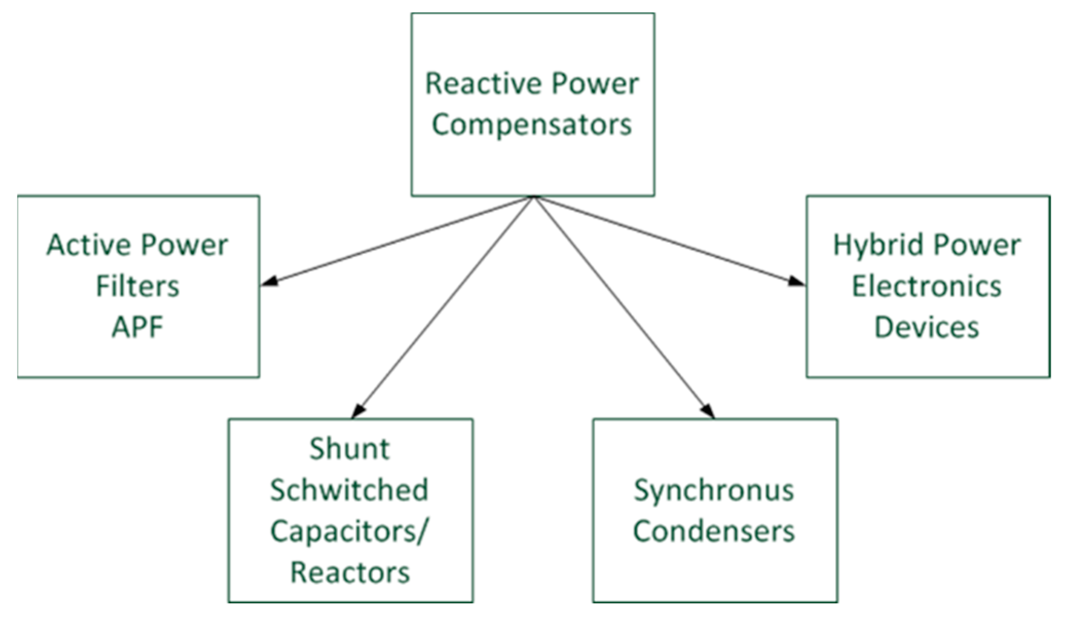
2.1. Classification of Reactive Power Compensation Systems

Currently applied solutions, enabling the improvement of the power factor consumed by electricity consumers, can be divided/classified into four groups of systems which are presented in Figure 1.
There are compensators of reactive power constructed on the basis of capacitors and energy chokes, active filters, synchronous motors, and hybrid systems consisting of capacitors and power electronics which are described in detail in references [6,7,8,9,10,11]. The most common in the industry for compensating reactive power are shunt compensators based on capacitors and energy chokes.
In most cases, reactive power regulation takes place on the principle of switching the maximum number of capacitor banks or reactors at a given moment or with a certain delay related to the sensitivity setting of the reactive power regulator [12]. This solution does not work in the case of fast-changing loads, where the battery is switched on for a moment which, in the next cycles, remains unavailable due to the need to discharge the energy accumulated inside to a safe voltage level. According to the Polish norm PN-EN 60,831 [13], the voltage on the discharged capacitor must drop to the level of U0 = 50 V in time no longer than tr = 60 s. This means that it is necessary to connect resistors to the compensation circuits, thanks to which the charge accumulated inside the capacitor is discharged. In addition, a large number of switches negatively affects the contactors connecting the batteries to the network. There occurs a contact burning phenomenon that leads to direct damage to the device and more frequent maintenance. It is also connected with an increase in the costs of using the compensation system.
The solution to this problem may be planning the compensation process based on the predicted reactive power waveform. An accurate forecast allows for the use of optimization algorithms supporting the regulator’s operation in the selection of the optimal use of available compensation levels. In this way it is possible to minimize the average value of reactive power consumed by the recipient and to limit the losses associated with excessively frequent switching of capacitor bank stages. In addition, the improvement of the capacitor battery driver’s operation enables it to be used to upgrade the existing batteries without the need to replace the entire device, or in other words to quick-change reactive power compensation systems. Similar solutions using time series prediction have been presented in the literature for prosumer management [14] and electricity consumption prediction [15]. The paper presents methods of prediction for reactive power consumption based on the structure of artificial neural networks. The impact of the size of the input vector and the structure of the neural network on the accuracy of time course estimation were tested. All the tests were carried out for actual data on the quality of electricity registered in an industrial building connected to a low-voltage network, located in Gliwice city in Poland.

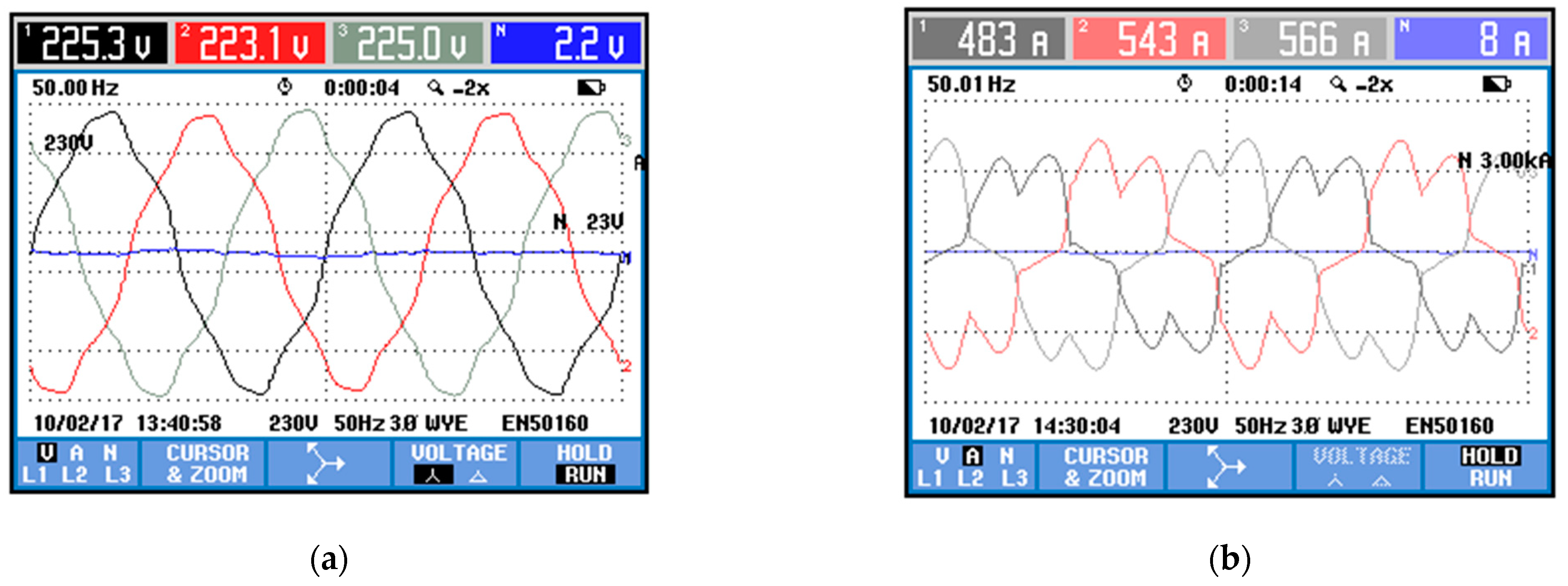
2.2. Research on a Real Object

The tested reactive power course was registered in an industrial building during auditing measurements using the Fluke 434 electrical power quality analyzer. Measurements of voltage and phase currents, whose oscillograms are shown in Figure 2, were made using the above-mentioned measuring device.
The effective values of phase voltages and currents in the analyzed supply network are at the level of UL = 223–225 V and IL = 483–543 A. Based on the shape of the waveform, it can be noticed that there are asymmetries and higher harmonics of both voltages and phase currents in the network. On the basis of the collected measurement data, the reactive power waveform was determined, which was aggregated with the averaging period TAVG equals 1 s. The recorded time curve is shown in Figure 3.
In the presented course, one can notice repeated two cycles related to the work of the plant. The first slow-moving one with amplitude Q1 = 70 kVAr and duration T1 = 80 s, and the second quick-change with amplitude Q2 = 100 kVAr and T2 = 15 s. This type of reactive power load causes considerable difficulties in the shunt capacitor bank, in which it reaches instantaneous activation of compensating stages and is followed by long periods of discharging.

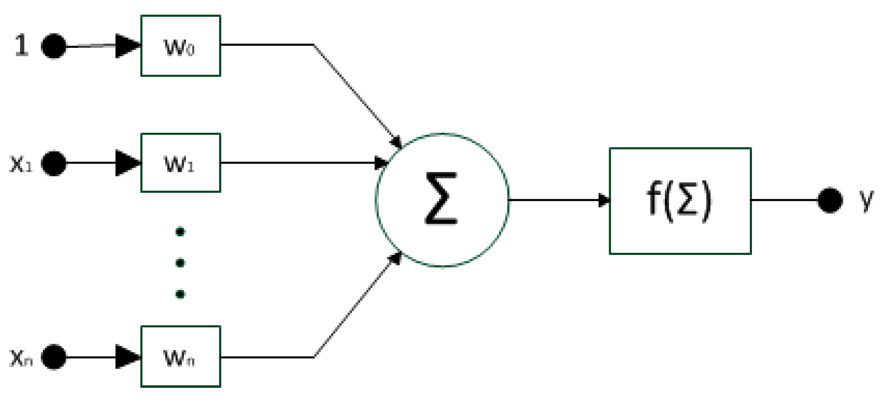
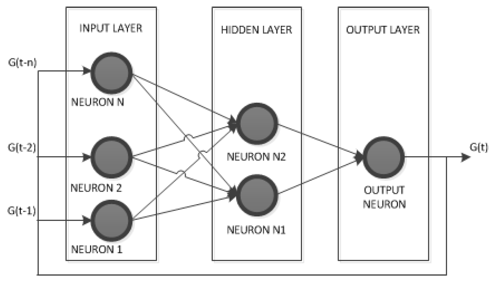
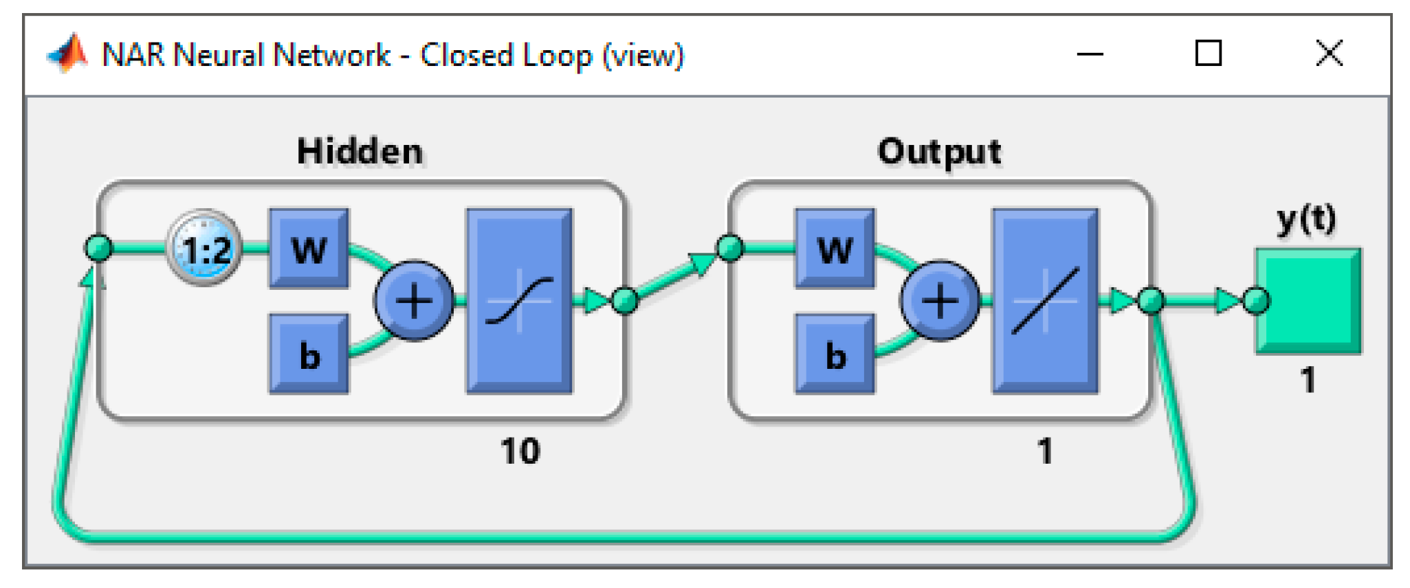
2.3. Artificial Neural Networks

Artificial neural networks are systems that directly refer to the behaviors occurring in the human nervous system. They are the basis for the construction of artificial intelligence systems. The basic element is the neuron, the structure of which is presented in Figure 4.
The classic model of the neuron given by McCulloch and Pitts [16] has n inputs (x1, …, xn) whose states (values) are multiplied by weighting factors (wo, …, wn). The partial products are then added together and transferred as the input value of the activation function, which on this basis calculates the neuron’s output state. The effects of a neuron action can be described mathematically as:
y = f ( i = 1 N w i x i ) ,
where xii-th inputs of the neuron, y—output of the neuron, wi—weighting factors of i-th input, f—neuron activation function, N—total number of inputs.
The activation function is selected depending on the problem being solved. Most often it has the form of a unit jump function, a linear or sigmoid function that can be written as:
f ( x ) = 1 1 + e α x     ,
where f(x)—value of activation function, x—the input value of the activation function, α—shape factor of the function.
The Artificial Neural Network (ANN) is a combination of artificial neurons grouped into layers capable of solving complex problems. ANN is mainly used for recognition and classification of images, filtration and prediction of time courses, and optimization and modeling of complex physical phenomena [17]. Due to the structure of the ANN networks, they can be divided/classified into one-way, recursive, and self-organizing ones. In the case of one-way networks, information flows in one direction from the entrance to the exit. In the recursive network, the inputs are given information that has already been processed by the network. The structure of self-organizing ANNs is not constant and is subject to change during the learning process of the network. Learning the neural network is based on the iterative change of neuron weighting factors and the evaluation of the approximate result by the network. In most cases, the learning process tends to minimize errors, resulting from the difference between the expected signal and the result of the action of the ANN [18].

3. Results, Implementation of Neural Networks

There are many papers presenting the implementation of artificial neural networks using the Python environment [19]. The authors decided to implement and test an ANN in a MATLAB environment with the Neural Network Toolbox libraries. Due to the nature of prediction (the need to determine subsequent samples only on the basis of archival samples), a nonlinear autoregressive Neural Network model (NAR) has been implemented. The diagram is shown in Figure 5. The NAR structure allows for the determination of the current G(t) signal sample based on the vector of archive samples G(t − 1, t − 2, …, Gn). In addition, programmable feedback from the network output enables long-term forecasting. To learn the network, the Levenberg–Marquardt algorithm was used, which combines the features of the fastest decline method and the Gauss–Newton method. The chosen learning algorithm is the fastest available algorithm for training one-way neural networks [18].
In order to determine the optimal structure of the NAR network in terms of the quality of predictions, simulations were carried out for networks with one hidden layer. In this layer, the number of N neurons from 1 to 30 with sigmoidal activation function was changed with the change of the input data vector n from 1 to 30. As learning data, the reactive power waveform presented in Figure 3 was used. The implemented exemplary network in a feedback system is presented in Figure 6.
The assessment of the selection of the optimal structure of the NAR network for the considered reactive power waveform was made on the basis of the percentage prediction error (E) for each of the predicted signal samples determined by the equation:
E = | y i p i y i | · 100 % ,
where E—percentage prediction error, yi—real value, pi—projected value.
The calculated E value was classified against four assessment criteria:
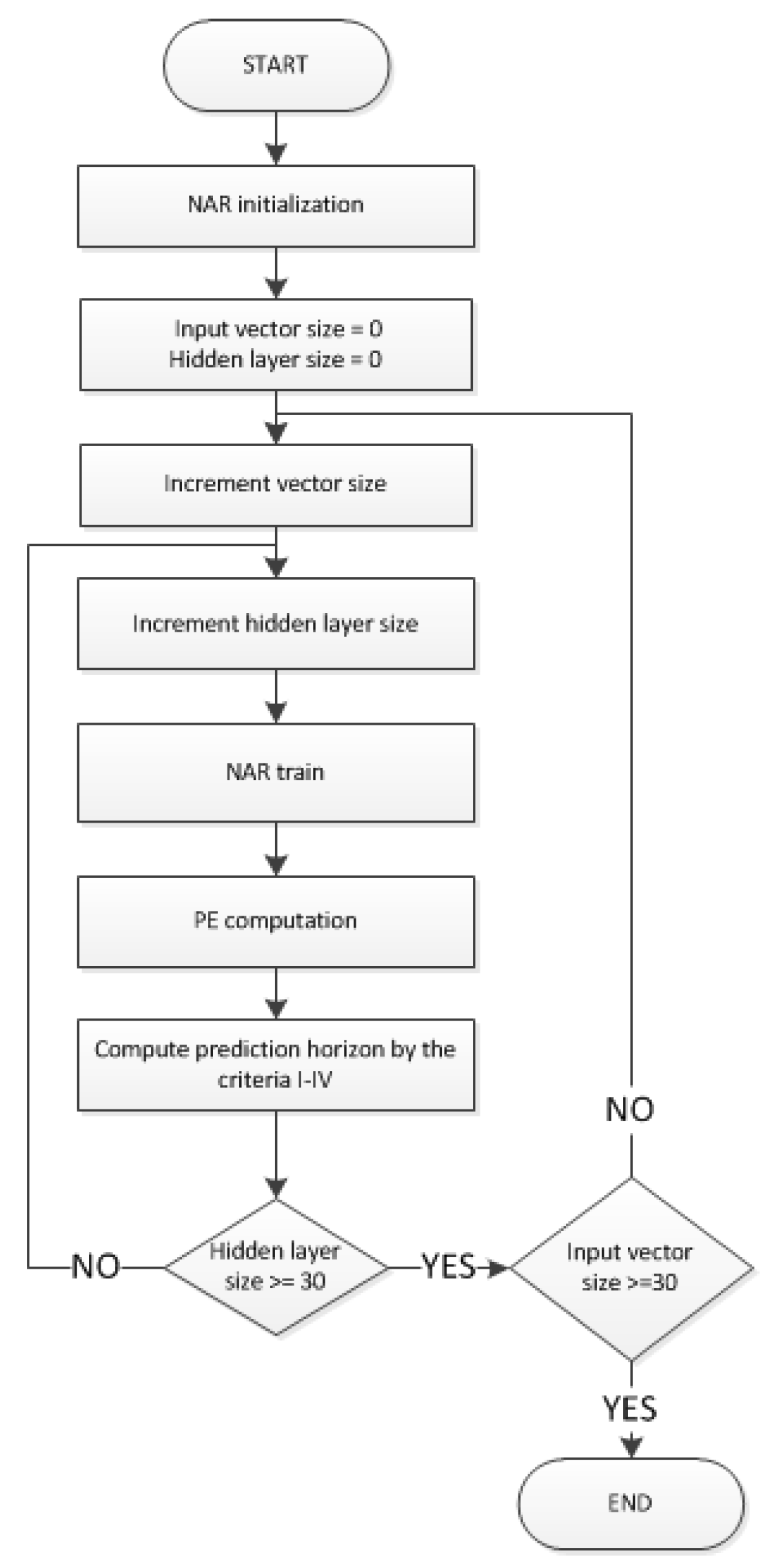
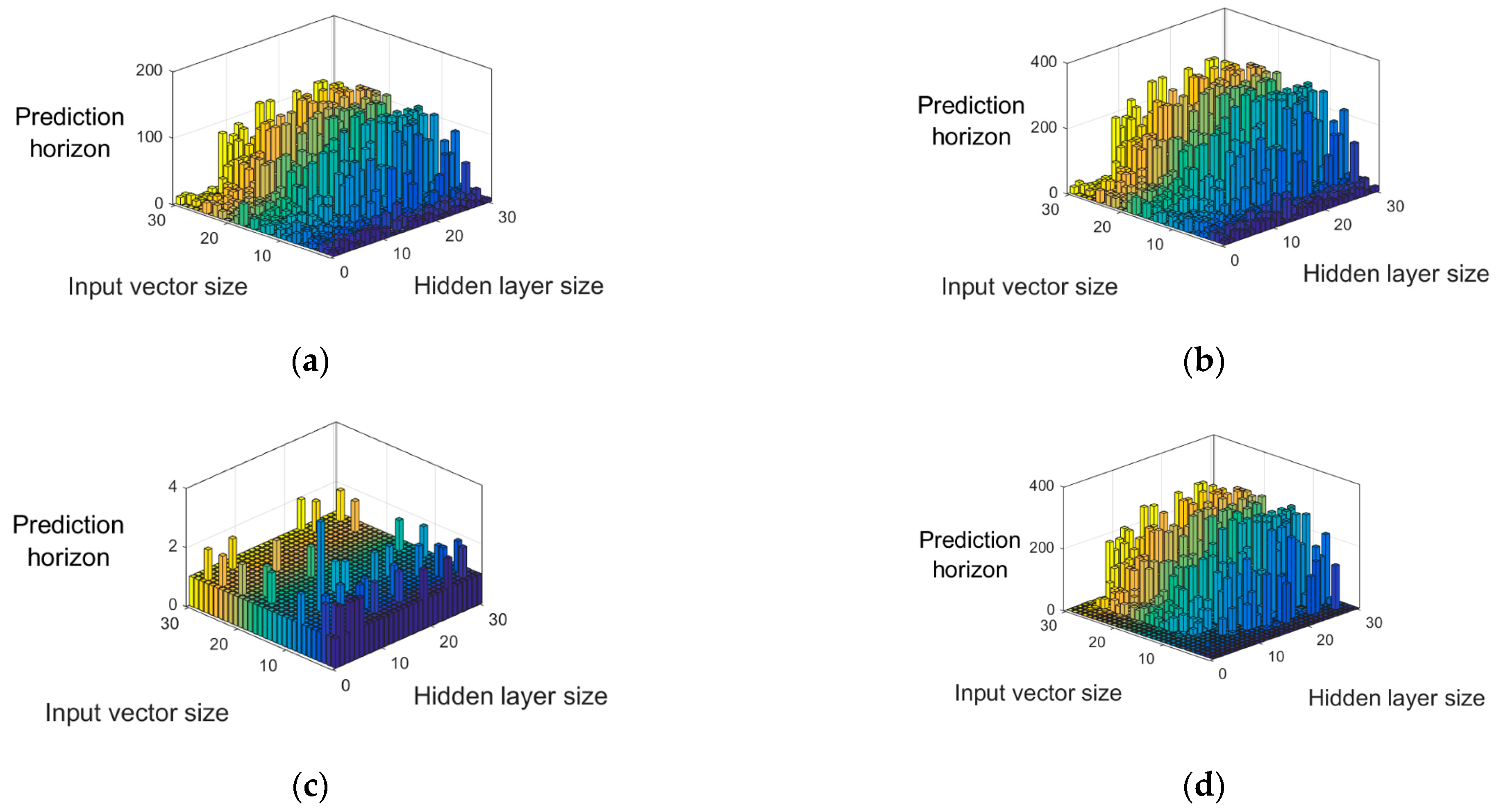
  • Criterion I consists in determining the maximum number of consecutive samples (the so-called prediction horizon) for which E does not exceed 5%;
  • Criterion II, as with criterion I, consists in determining the maximum prediction window for E not exceeding 2%;
  • Criterion III consists in determining the number of samples for which E does not exceed 5%;
  • Criterion IV consists in determining the number of samples for which E does not exceed 2%.
The simulation algorithm for determining the optimal structure of the NAR network for the problem of prediction of reactive power is presented in Figure 7. It consists in network initialization and subsequent changes in the number of hidden layer neurons and the size of the input vector. In the next steps, network training, calculation of prediction error, and evaluation of the forecast against criteria I–IV are performed.
The values obtained for the given assessment criteria are presented in Figure 8, on the basis of which it can be noticed that small amounts of input signal samples and hidden layer neurons generate a very short prediction horizon. In the case of increasing their amount, N = 5 neurons and n = 5 samples of the input vector can be assumed as the limit. Subsequently, a gradual increase in the correct mapping of the original course occurs. Too many neurons of the hidden layer, in turn, lead to erroneous forecasts caused by the phenomenon of overfitting the neural network [20,21].
Unfortunately, the prediction horizon with the 2% error limit described as criterion II is very short, and its maximum value for the entire experiment is three samples. In the case of a 5% error limit, the prediction horizon lengths are much larger and vary from 3 to 178 samples. The assessment of the mapping error using criteria III and IV made it possible to examine the prediction error for a rigidly determined prediction horizon equal to n = 292 of the sample. On the basis of the comparison with criteria I and II, it can be seen that the number of forecasted samples whose error is below a certain level is much higher. This means that in addition to temporary increases in the mapping error, it returns to the values admissible by the criterion. The system with N = 7 neurons of the hidden layer and n = 14 samples of the input vector was selected as the best structure for the NAR network. The values that the given system has obtained in each of the criteria are presented in Table 1.
The comparison of the original and forecasted courses for the selected neural network structure is presented in Figure 9. The prediction E course and the graph of dependence of samples measured from the predicted ones are also presented. According to the values in Table 1, the course of the error to about t = 3 min and 27 s reaches values below 5%. This accuracy of the reactive power rating forecast is completely sufficient to conduct further research on the predictive reactive power controller for bypass compensation circuits.

4. Conclusions

In this article, the possibility of adapting artificial neural networks to the prediction of fast-changing reactive power time passages is presented. The NAR (Nonlinear Autoregressive Neural Network) structure was used for this purpose. It has been shown that this structure, based on archival data, allows for forecasting the reactive power course, useful for optimal planning of reactive power compensation strategies. Thus, comparison of the original and forecasted courses confirms that it is possible to forecast the reactive power course, useful for optimal planning of reactive power compensation strategies. The influence of the quantity of hidden layer neurons and the size of the input data vector on the length of the prediction horizon were investigated/studied at the determined allowable forecast error values. Futher research should focus on the determination of computational complexity and implementation costs of NARs in real reactive power controllers. This work is the starting point which will serve as the basis for optimizing the control process of shunt compensators.

Author Contributions

Conceptualization, D.B. and T.T.; methodology, D.B. and T.T.; software, D.B., T.T. and M.R.; validation, T.T., M.S. and M.R.; formal analysis, D.B.; investigation, D.B.; resources, writing—original draft preparation, D.B., T.T. and M.S.; writing—review and editing, T.T. and M.S. All authors have read and agreed to the published version of the manuscript.

Funding

This research received no external funding.

Institutional Review Board Statement

Not applicable.

Informed Consent Statement

Not applicable.

Data Availability Statement

Not available.

Conflicts of Interest

The authors declare no conflict of interest.

References

  1. Anderson, H.C.; Al Hadi, A.; Jones, E.S.; Ionel, D.M. Power factor and reactive power in us residences—Survey and EnergyPlus modeling. In Proceedings of the 2021 10th International Conference on Renewable Energy Research and Application (ICRERA), Istanbul, Turkey, 26–29 September 2021; pp. 418–422. [Google Scholar] [CrossRef]
  2. Wang, Y.; Wang, T.; Zhou, K.; Cao, K.; Cai, D.; Liu, H.; Zhou, C. Reactive power optimization of wind farm considering reactive power regulation capacity of wind generators. In Proceedings of the 2019 IEEE Innovative Smart Grid Technologies—Asia (ISGT Asia), Chengdu, China, 21–24 May 2019; pp. 4031–4035. [Google Scholar] [CrossRef]
  3. Trawiński, T.; Szczygieł, M.; Kołton, W.; Kłapyta, G.; Hojeński, M.; Morański, J.; Ozdoba, K. Analysis of electrical energy consumption in chosen company in the context of the modern methods of reactive power compensation. Pract. Nauk. Pśl. Elektr. 2015, 3, 65–78. (In Polish) [Google Scholar]
  4. Huang, H.; Nie, J.; Li, Z.; Wang, K. Distributed dynamic reactive power support system based on DFIGs. In Proceedings of the 2019 IEEE 8th International Conference on Advanced Power System Automation and Protection (APAP), Xi’an, China, 21–24 October 2019; pp. 283–288. [Google Scholar] [CrossRef]
  5. Pournazarian, B.; Sangrody, R.; Saeedian, M.; Gomis-Bellmunt, O.; Pouresmaeil, E. Enhancing microgrid small-signal stability and reactive power sharing using anfis-tuned virtual inductances. IEEE Access 2021, 9, 104915–104926. [Google Scholar] [CrossRef]
  6. Huang, S.; Yao, R.; Huang, C.; Wang, R.; Li, X.; Yang, H. Reactive power optimization analysis of HVDC converter station based on RTDS simulation. In Proceedings of the 2020 4th International Conference on HVDC (HVDC), Xi’an, China, 6–9 November 2020; pp. 439–442. [Google Scholar] [CrossRef]
  7. Buła, D.; Pasko, M. Dynamical properties of hybrid power filter with single tuned passive filter. Przegląd Elektrotech. 2011, 1, 91–95. [Google Scholar]
  8. Buła, D.; Pasko, M. Stability analysis of hybrid active power filter. Bull. Pol. Acad. Sci. Tech. Sci. 2014, 62, 279–286. [Google Scholar] [CrossRef] [Green Version]
  9. Das, J.C. Passive filters–potentialities and limitations. IEEE Trans. Ind. Appl. 2004, 40, 232–241. [Google Scholar] [CrossRef]
  10. Baggini, A. Handbook of Power Quality; John Wiley & Sons: Hoboken, NJ, USA, 2008. [Google Scholar]
  11. Strzelecki, R.; Supronowicz, H. Power Factor in AC Power Systems and Methods for Its Improvement; Warsaw University of Technology Publishing House: Warszawa, Poland, 2000. (In Polish) [Google Scholar]
  12. Hanzelka, Z. Jakość Dostawy Energii Elektrycznej. Zaburzenia Wartości Skutecznej Napięcia; Wydawnictwo AGH: Kraków, Poland, 2013. (In Polish) [Google Scholar]
  13. Polish Norm PN-EN 60831-1:2014-10; Kondensatory Samoregenerujące do Równoległej Kompensacji Mocy Biernej w Sieciach Elektroenergetycznych Prądu Przemiennego o Napięciu Znamionowym do 1000 V Włącznie. Sektor Elektryki: Warszawa, Poland, 2014. (In Polish)
  14. Irtija, N.; Sangoleye, F.; Tsiropoulou, E. Contract-Theoretic Demand Response Management in Smart Grid Systems. IEEE Access 2020, 8, 184976–184987. [Google Scholar] [CrossRef]
  15. Tomcala, J. Towards Optimal Supercomputer Energy Consumption Forecasting Method. Mathematics 2021, 9, 2695. [Google Scholar] [CrossRef]
  16. McCulloch, W.S.; Pitts, W. A logical calculus of the ideas immanent in nervous activity. Bull. Math. Biophys. 1943, 5, 115–133. [Google Scholar] [CrossRef]
  17. Włas, M. Zastosowanie algorytmów sztucznych sieci neuronowych do prognozowania zużycia energii elektrycznej. In Zeszyty Naukowe Wydziału Elektrotechniki i Automatyki Politechniki Gdańskiej; Politechniki Gdańskiej: Gdańsk, Poland, 2016; Volume 51, pp. 217–220. (In Polish) [Google Scholar]
  18. Nocoń, A. Metody CAD i AI W inżynierii Elektrycznej; Wydawnictwo WNT: Warsaw, Poland, 2018. (In Polish) [Google Scholar]
  19. Siebert, J.; Gross, J.; Schroth, C.H. A Systematic Review of Python Packages for Time Series Analysis; Fraunhoffer-Institure fur Exerimentelles Software Engineering: Kaiserslautern, Germany, 2021. [Google Scholar]
  20. Łęski, J. Systemy Neuronowo-Rozmyte; Wydawnictwo WNT: Warsaw, Poland, 2008. [Google Scholar]
  21. Jeżyk, T.; Tomczewski, A. Krótkoterminowe prognozowanie zużycia energii elektrycznej z wykorzystaniem sztucznej sieci neuronowej. Pozn. Univ. Technol. Acad. J. 2014, 79, 121–130. (In Polish) [Google Scholar]
Figure 1. Classification of reactive power compensation devices.
Electronics 11 02005 g001
Figure 2. Oscillograms representing: (a) voltages; (b) current waveforms in the tested object.
Electronics 11 02005 g002
Figure 3. The total time curve of consumed reactive power.
Electronics 11 02005 g003
Figure 4. McCulloch and Pitts neuron model.
Electronics 11 02005 g004
Figure 5. Diagram of a non—linear autoregressive network (NAR).
Electronics 11 02005 g005
Figure 6. Diagram of a two-layer neural network in MATLAB.
Electronics 11 02005 g006
Figure 7. The simulation algorithm implemented in the MATLAB program.
Electronics 11 02005 g007
Figure 8. Simulation results for individual evaluation criteria: (a)—criterion I, (b)—criterion III, (c)—criterion II, (d)—criterion IV.
Electronics 11 02005 g008
Figure 9. Simulation results for N = 7 neurons, n = 14 samples of the input vector: (a)–measured and predicted, (b)–prediction error, and (c)–predicted vs. measured reactive power.
Electronics 11 02005 g009
Table 1. The values of the assessment criteria for the structure with N = 7 neurons and G = 14 samples of the input vector.
Assessment CriteriaValue
Criterion I217
Criterion II2
Criterion III217
Criterion IV92
Publisher’s Note: MDPI stays neutral with regard to jurisdictional claims in published maps and institutional affiliations.

