Article

Fusion of Infrared and Visible Images Based on Optimized Low-Rank Matrix Factorization with Guided Filtering

1
Department of UAV, Army Engineering University, Shijiazhuang 050003, China
2
Department of Electronic and Optical Engineering, Army Engineering University, Shijiazhuang 050003, China
3
Equipment Simulation Training Center, Army Engineering University, Shijiazhuang 050003, China
*
Authors to whom correspondence should be addressed.
Electronics 2022, 11(13), 2003; https://doi.org/10.3390/electronics11132003
Submission received: 9 June 2022 / Revised: 22 June 2022 / Accepted: 25 June 2022 / Published: 26 June 2022
(This article belongs to the Section Computer Science & Engineering)

Abstract

:
In recent years, image fusion has been a research hotspot. However, it is still a big challenge to balance the problems of noiseless image fusion and noisy image fusion. In order to improve the weak performance and low robustness of existing image fusion algorithms in noisy images, an infrared and visible image fusion algorithm based on optimized low-rank matrix factorization with guided filtering is proposed. First, the minimized error reconstruction factorization is introduced into the low-rank matrix, which effectively enhances the optimization performance, and obtains the base image with good filtering performance. Then using the base image as the guide image, the source image is decomposed into the high-frequency layer containing detail information and noise, and the low-frequency layer containing energy information through guided filtering. According to the noise intensity, the sparse reconstruction error is adaptively obtained to fuse the high-frequency layers, and the weighted average strategy is utilized to fuse the low-frequency layers. Finally, the fusion image is obtained by reconstructing the pre-fused high-frequency layer and the pre-fused low-frequency layer. The comparative experiments show that the proposed algorithm not only has good performance for noise-free images, but more importantly, it can effectively deal with the fusion of noisy images.

1. Introduction

Infrared and visible image fusion is an important part of the image processing field, and its main purpose is to merge the complementary information in different images into one picture through technical algorithms [1]. Since the fused image can mostly maintain the significant features and energy information from various sensors, the fusion result can be utilized by subsequent processing tasks or decision-making assistance. Therefore, it can provide strong support in target detection and tracking, military fields, computer vision, remote sensing, and medical treatment [2].
In recent years, convolutional neural networks have developed rapidly and have been widely used in many fields [3]. Since deep learning can effectively extract and express salient features, it has developed rapidly in the field of image fusion. Liu et al. [4] proposed a convolutional neural network (CNN)-based infrared and visible image fusion method, using a twin convolutional network to obtain a weight map that integrates pixel activity information from two source images. Liu et al. [5] proposed a new method called convolutional sparse representation, which combines the advantages of convolutional neural networks and sparse representation for image fusion. Luo et al. [6] proposed an infrared and visible image fusion method based on Nonsubsampled Contourlet Transform (NSCT) and stacked autoencoders. The image was decomposed into high-frequency and low-frequency layers using NSCT, and the low-frequency coefficients were calculated by stacking autoencoders to achieve image fusion. Hui et al. [7] used a deep learning network to extract salient features to obtain a better image fusion performance. Daniela et al. [8] designed an automated solution for facial feature recognition, enabling further applications of infrared and visible image fusion. However, judging from the fusion results of these papers, the performance of deep learning-based algorithms is not always better than traditional algorithms, and the results are even worse due to insufficient training samples. Moreover, due to the high computational complexity, powerful hardware support is required. In addition, due to the lack of actual ground data, both infrared and visible deep learning-based methods belong to unsupervised learning. Therefore, compared with the traditional method, the deep learning methods only rely on the composition of the network architecture and the design of the loss function, and it is difficult to obtain an overwhelming fusion result.
So far, the fusion methods based on multi-scale decomposition have been deeply and meticulously researched, and a good fusion performance has been achieved. For example, Singh et al. [9] designed two different infrared and visible image fusion schemes in the wavelet domain and feature space domain, respectively, and achieved good results in practice. Wang et al. [10] proposed an image fusion method based on an improved pulse-coupled neural network (PCNN) and multi-scale decomposition, which can produce good visual effects. Zhou et al. [11] proposed a new hybrid multi-scale image fusion method based on gradient-guided filtering. The fusion result can fully show the advantages in contrast and detail preservation. Ma et al. [12] proposed a multi-scale decomposition image fusion method through the combination of rolling guided filters and Gaussian filters. In order to improve the fusion performance of the detail layer, this method also proposed an optimized weighted least squares scheme. To overcome the limitations of the edge-preserving filter and reduce the artifacts at the edges of the image, Zhang et al. [13] used a new edge-preserving technology to achieve image fusion, and the co-occurrence filter can extract and fuse images. Therefore, a good image fusion effect was obtained. Duan et al. [14] proposed a new decomposition method called the multi-scale decomposition of the double exponential edge preservation smoother. This method can fully extract multi-scale structural information, and has good performance in terms of natural visual effects and detail preservation.
Most of the algorithms mentioned above ignore a key issue. Generally, the image fusion performance obtained by different image sensors is easily affected by imaging equipment and environmental factors, and there may be some noise in the images. However, traditional algorithms cannot take into account the fusion of noisy images and noise-free images simultaneously. To solve this problem, a new image fusion algorithm based on optimized low-rank matrix decomposition and guided filtering based on the traditional algorithm is proposed, which can effectively remove the noise in the image and obtain a good fusion image. In addition, the proposed algorithm also has good edge and detail preservation ability as well as good robustness. The main contributions of this article are as follows:
(1) To achieve a good denoising performance, the minimized error reconstruction factor is introduced. The effect of low-rank matrix decomposition is optimized, and image denoising can be achieved through update iteration;
(2) In order to effectively separate the noise information and energy structure information from the source image, guided filtering is utilized to decompose the source image at two scales. Among them, due to the optimization of low-rank matrix decomposition, an image with good denoising performance can be obtained, which can be utilized as a guided image, and then the good filtering performance of guided filtering can be utilized to better decompose the source image into a high-frequency layer with noise information and a low-frequency layer with energy structure information;
(3) In order to realize the denoising fusion of the high-frequency layer, an adaptive sparse error reconstruction method is proposed, which can adaptively change the denoising ability according to the intensity of the noise, avoiding excessive denoising or insufficient denoising.
The rest of this paper is organized as follows: Section 2 introduces some key theoretical algorithms used in this paper; Section 3 introduces the proposed algorithm; Section 4 introduces the comparative test and parameter setting; finally, the conclusion is described in Section 5.

2. Key Theories

2.1. Low-Rank Matrix Factorization Based on Minimizing Errors

The matrix D can be regarded as the low-rank part A and the sparse part E which can be modeled as the following optimization problem [15]:
min A , E rank ( A ) + λ E 0 , s . t .   D = A + E
where rank ( A ) and E 0 are both nonlinear and non-convex, so optimization is difficult.
Therefore, it is necessary to use the rank and norm of the matrix to perform convex relaxation, so that the above formula is relaxed into the following convex optimization problem. In order to obtain a better optimization effect, the minimum error reconstruction factor β is introduced, and the above formula becomes:
min A , E A * + λ E 1 , 1 + β D A E 1 , 1 , s . t .   D = A + E
Solving convex optimization problems can be optimized by an iterative threshold algorithm, accelerated near-end gradient method, dual method, etc. In this paper, an augmented Lagrange multiplier algorithm (alternating direction multiplier method [16]) is used for optimization. First, construct the augmented Lagrange function:
L ( A , E , Y , u ) = A * + λ E 1 , 1 + β D A E 1 , 1 + < Y , D A E > + u 2 D A E F 2
When Y = Y k , u = u k , the alternate algorithm is used to solve the optimization problem:
min A , E L ( A , E , Y k , u k )
The exact Lagrange multiplier method is utilized to alternately iterate the matrices A and E until the termination condition is met. If E = E k + 1 j , then
A k + 1 j + 1 = arg min A L ( A , E k + 1 j , Y k , u k ) = arg min A A * + β D A E k + 1 j 1 , 1 + u k 2 A ( D E k + 1 j + Y k u k ) F 2 = D 1 u k , β ( D E k + 1 j + Y k u k )
Then update the matrix E according to A k + 1 j + 1 :
E k + 1 j + 1 = arg min A L ( A k + 1 j + 1 , E , Y k , u k ) = arg min A λ E 1 , 1 + β D A k + 1 j + 1 E 1 , 1 + u k 2 E ( D A k + 1 j + 1 + Y k u k ) F 2 = S 1 u k , β ( D A k + 1 j + 1 + Y k u k )
Let A k + 1 * and E k + 1 * be the exact values of A k + 1 j + 1 and E k + 1 j + 1 , respectively, then the update formula of matrix Y is:
Y k + 1 = Y k + u k ( D A k + 1 * E k + 1 * )
The parameter u k can be updated as follows:
u k + 1 = { ρ u k     , u k E k + 1 * E k * F D F < ε u k         , o t h e r w i s e  
where ρ > 1 is a constant, and ε > 0 is a small positive number.
The above-mentioned accurate Lagrange multiplier method (ALM) requires multiple updates in the inner loop and performs multiple singular value decompositions. Therefore, an inaccurate Lagrange multiplier method is proposed, which does not require the exact solution of min A , E L ( A , E , Y k , u k ) before the external loop starts; that is, the inner loop of the ALM method is removed, and the update formula becomes the following form:
A k + 1 = arg min A L ( A , E k + 1 , Y k , u k ) = D 1 u k , β ( D E k + 1 + Y k u k )
E k + 1 = arg min E L ( A k + 1 , E , Y k , u k ) = S λ u k , β ( D A k + 1 + Y k u k )
where D 1 u k , β and S λ u k , β are singular value threshold operators and soft threshold operators, respectively.

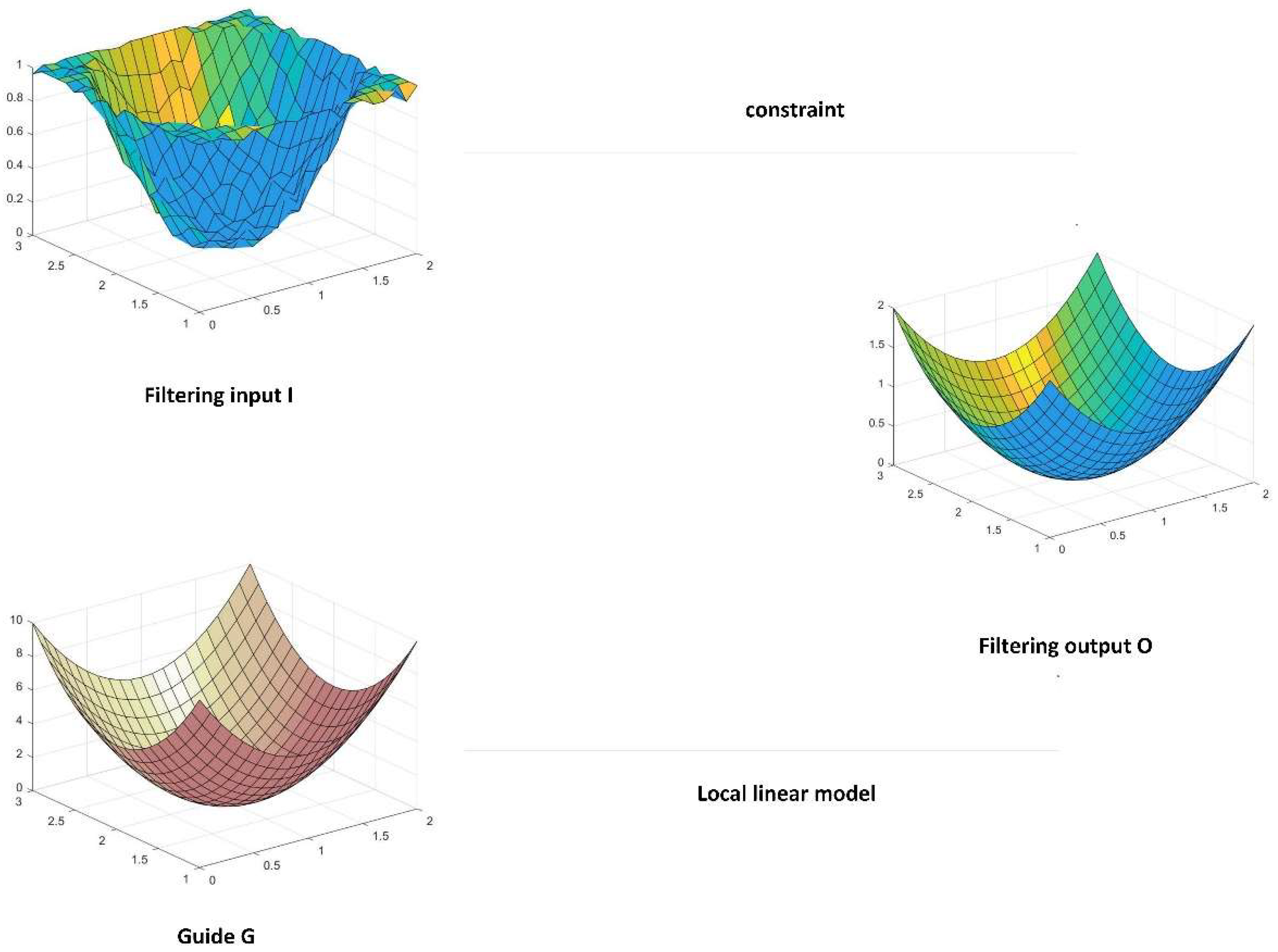
2.2. Guided Filtering
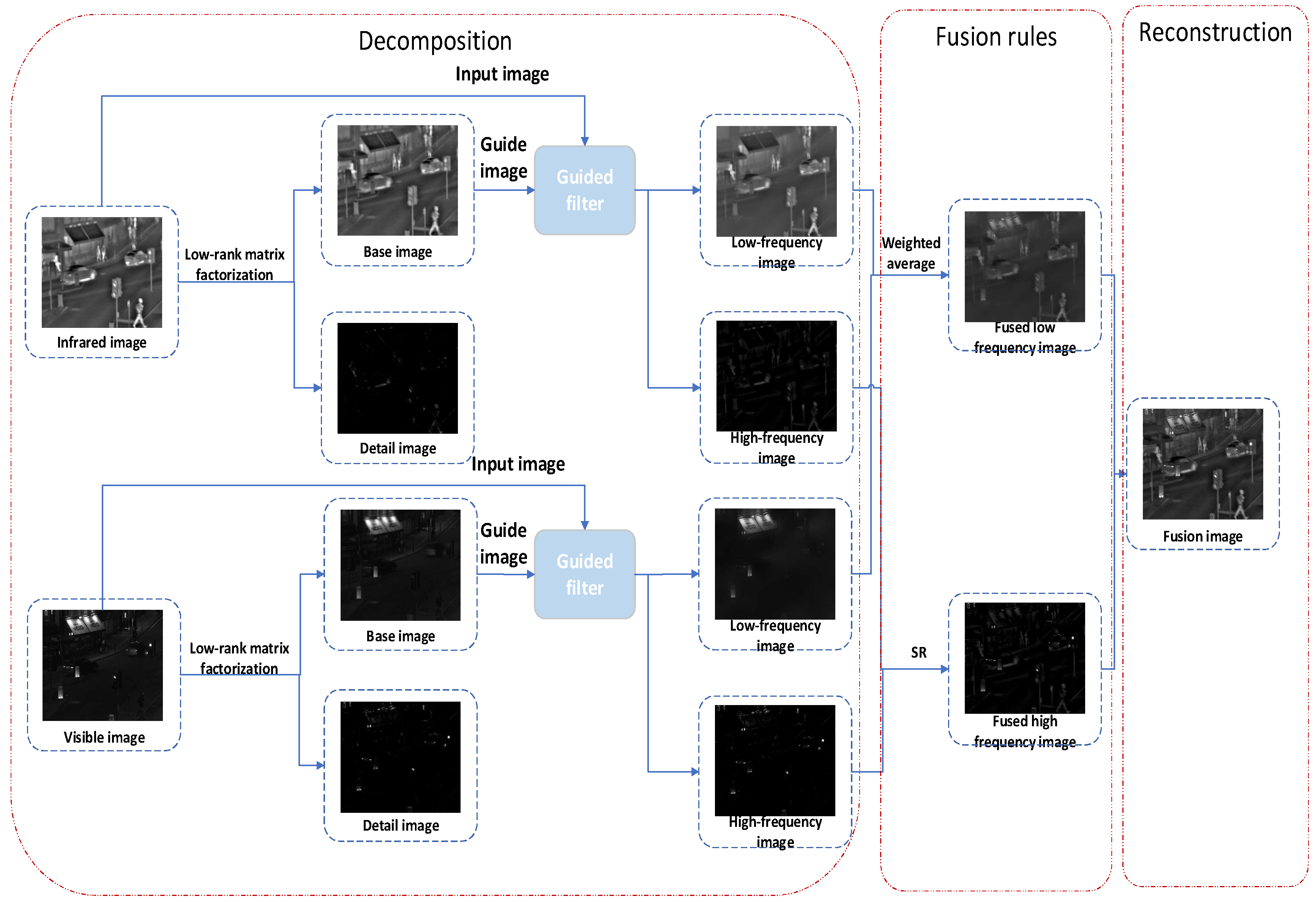
Traditional edge-preserving smoothing filters including the weighted least squares filter [17] or bilateral filter [18] are widely utilized in the field of image processing, which can avoid ringing artifacts and achieve the effect of not blurring the edges during the decomposition process. Guided filtering [19] also belongs to an edge-preserving filtering algorithm, which can obtain an edge-preserving smooth image through a guided image. Guided filtering is a local linear model of guided image G i and filter output O i :
O i = p n G i + q n , i θ n
where p n and q n are constants in the window θ n at the pixel n . The idea of optimized regression is used to solve I o . Then the cost function is defined, and a regular term ϵ is added to the cost function through the ridge regression method to prevent overfitting.
E ( p n , q n ) = i θ n ( ( p n G i + q n I i ) 2 + ϵ p n 2 )
where I i is the input image. Through this formula, p n and q n that minimize E ( p n , q n ) can be obtained
p n = 1 | α | i ϵ θ n G i I i θ n I ^ n σ n 2 + ϵ
q n = I ^ n p n θ n
where θ n and σ n 2 are the mean value and variance of I in θ n , respectively, I ^ n is the mean value of I in θ n , and | α | is the number of pixels in θ n . The p n and q n in each window are obtained by traversing the image through the window. However, each pixel may be contained in multiple windows, which leads to multiple calculations of p n and q n . Therefore, in order to simplify the calculation, take the average value p ^ n , q ^ n of p n and q n , and then obtain:
O i = p ^ n G i + q ^ n
Guided filtering is different from most filtering methods in that it requires direct convolution, and its calculation time has nothing to do with the filter parameters. Because of its good edge retention and structure transfer characteristics, it is widely utilized in the fields of image decomposition, image smashing, and image fusion. Figure 1 is a schematic diagram of guided filtering.

3. Fusion Framework

In order to solve the problem of effectively retaining details while denoising, a new fusion model is introduced. Different from traditional decomposition methods, the source image is first denoised and decomposed by using an optimized low-rank matrix in order to achieve better denoising effect. At this time, the source image is decomposed into base component and detail component, and most of the disturbance can be completely preserved in the detail component. Then the base component is used as the guide image, the source image is used as the input image, and the source image is decomposed into a high-frequency layer and a low-frequency layer through a guided filter. The high-frequency layer contains detail and noise components, and the low-frequency layer contains energy and structure information. Different fusion methods are introduced to obtain pre-fusion layers based on the characteristics of the two layers. Among them, for the high-frequency layer fusion, fusion denoising is effectively realized by combining the relationship between sparse representation and noise intensity; for the low-frequency layer, a weighted average fusion strategy is used for pre-fusion. Finally, the final fusion image is realized by reconstructing the two pre-fusion layers. Figure 2 shows the main flow of the algorithm in this paper.

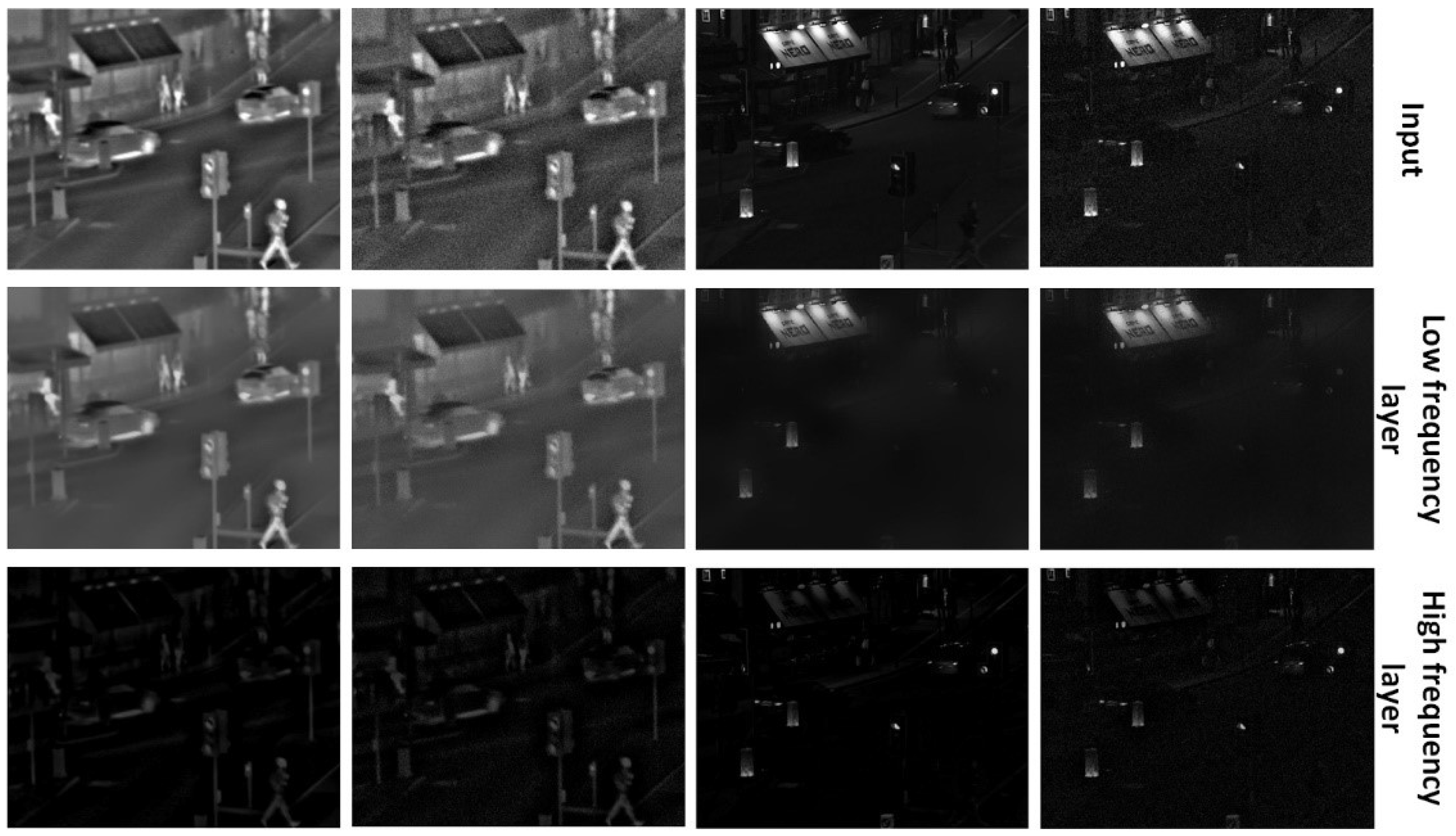
3.1. The Decomposition Model

In order to separate the noise in the source image in a targeted manner, using the optimized low-rank matrix’s better denoising effect, first process the source image:
( I n b , I n d ) = L R F ( I n , μ , λ )
where I n is the n th source image, n { 1 , 2 , , N } , μ and λ are the iteration error and the number of iterations, respectively, L R F ( · ) is the low-rank matrix factorization operator, and I n b is the base component after the noise removal. Next, I n is used as the input image, I n b is used as the guide image, and the low-frequency layer of the image is obtained through the guiding filter:
I n l = G F ( I n , I n b , σ s , σ r )
where σ s , σ r are filter parameters, G F ( · ) is the guided filter operator, and I n l represents the low-frequency layer of I n . After the guided filtering, most of the noise has been removed from the image, and the important details and structural information in the image are retained in the low-frequency layer. The high-frequency layer of the image can be obtained by the following formula:
I n h = I n I n l
Each group of images in Figure 3 contains a noise-free image and a noisy image with σ = 20 . These two groups of images test the reliability of the proposed decomposition model, especially for noisy images. It can be seen from Figure 3:
(1) After decomposition by the proposed algorithm, most of the noise and details are preserved to the high-frequency layer. At the same time, it can be seen that some details still exist in the low-frequency layer;
(2) The low-frequency layer produced by noise-free and noisy images is very similar; that is, the noise information almost completely exists in the high-frequency layer.

3.2. Fusion Rules

3.2.1. High-Frequency Layers Pre-Fusion

The method based on SR can well realize the fusion denoising of the detail layers. It includes two stages: dictionary learning and sparse representation. In the first step, the high-frequency layer of training data is generated by Equation (17), 8 × 8 blocks are collected from detail images, and the final training collection is constructed. The Kernel-based singular value decomposition (KSVD) [20] algorithm can be used to obtain a complete dictionary D. In the second step, an 8 × 8 block of each source image is taken and normalized. To obtain SR parameters of high-frequency layers, an Orthogonal Matching Pursuit (OMP) [21] algorithm is utilized by Equation (18):
min α n k α n k 0 , s . t . V n k D α n k 0 < ε
where V n k is the k -th block of I n , and α n k is the related sparse vector. ε is the sparse reconstruction error, represented as:
ε = { P ,                                             σ = 0 0.005 + 8 E σ , σ > 0
where σ is the Gaussian standard deviation, P is a constant, and E > 0 influences ε when σ > 0 . Next the “absolute-maximum” is utilized to obtain fusion sparse representation coefficients:
α F h k = α n ^ k ,   n ^ = arg max n { α n k 1 | n = 1 , 2 , , N }
The fusion high-frequency vector α ¯ F h k can be obtained by:
α ¯ F h k = D α F h k
Finally, the fusion high-frequency layer is obtained by reshaping each α ¯ F h k into 8 × 8 blocks and then arranging them according to the initial location to generate the pre-fused F h .

3.2.2. Low-Frequency Layers Pre-Fusion

The low-frequency layer of the source image contains more global structural information and energy information. Therefore, this paper uses a weighted average strategy [22] for low-frequency layer fusion:
F l = ω 1 I 1 h + ω 2 I 2 h
where ω 1 and ω 2 represent the weight value. In order to maintain the global structure and energy information and reduce redundant information, let ω 1 = 0.5 and ω 2 = 0.5 .
After obtaining these two pre-fusion components, the final fusion image F is:
F = F h + F l

4. Discussion

In this section, after setting the parameters of the proposed algorithm, a comparative experiment is carried out, including the experiment of the noiseless image and the experiment of the image with noise. Qualitative and quantitative analyses were carried out, respectively.

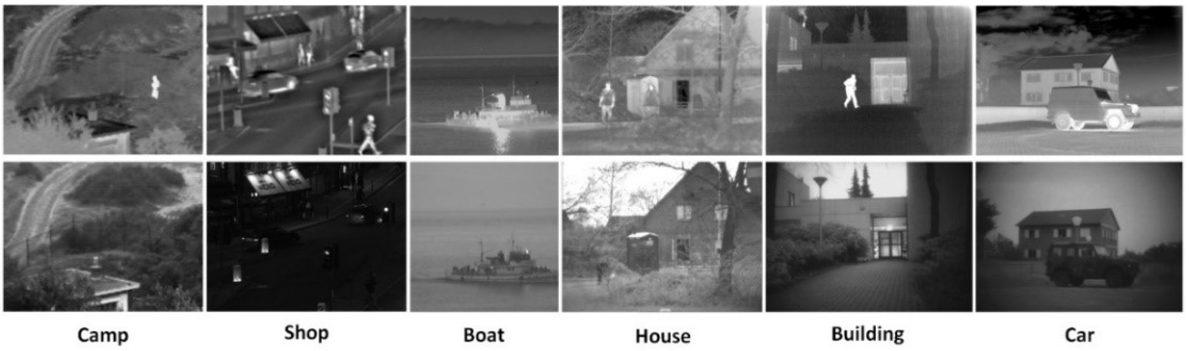
4.1. Experimental Setup

The experimental dataset is selected from the website https://figshare.com/articles/TN_Image_Fusion_Dataset/1008029 (accessed on 15 May 2022) to verify the proposed algorithm. Six pairs of images are shown in Figure 4. Five recent methods are compared in the same experimental environment for verification, including CBF [23], CNN [4], GTF [24], IFEVIP [25], and TIF [26]. Furthermore, the fusion performance is quantitatively evaluated by six indicators, including entropy (EN) [27], edge information retention ( Q A B / F ) [28], Chen-Blum’s index ( Q C B ) [29], mutual information (MI) [30], structural similarity (SSIM) [31], and peak signal-to-noise ratio (PSNR) [32].
EN is used to measure the amount of information contained in the source image in the fusion image. Q A B / F utilizes local metrics to estimate how well salient information from source images is represented in fused images. Q C B is used as a human visual evaluation index to measure the quality of fused images. MI is used to measure the amount of information transferred from the source image into the fused image. SSIM is used to measure the structural similarity between the fused image and the source image. PSNR is used to measure the ratio between the effective information of the image and the noise, which can reflect whether the image is distorted. In summary, these metrics are chosen to evaluate the fused images obtained by the proposed algorithm from different perspectives.

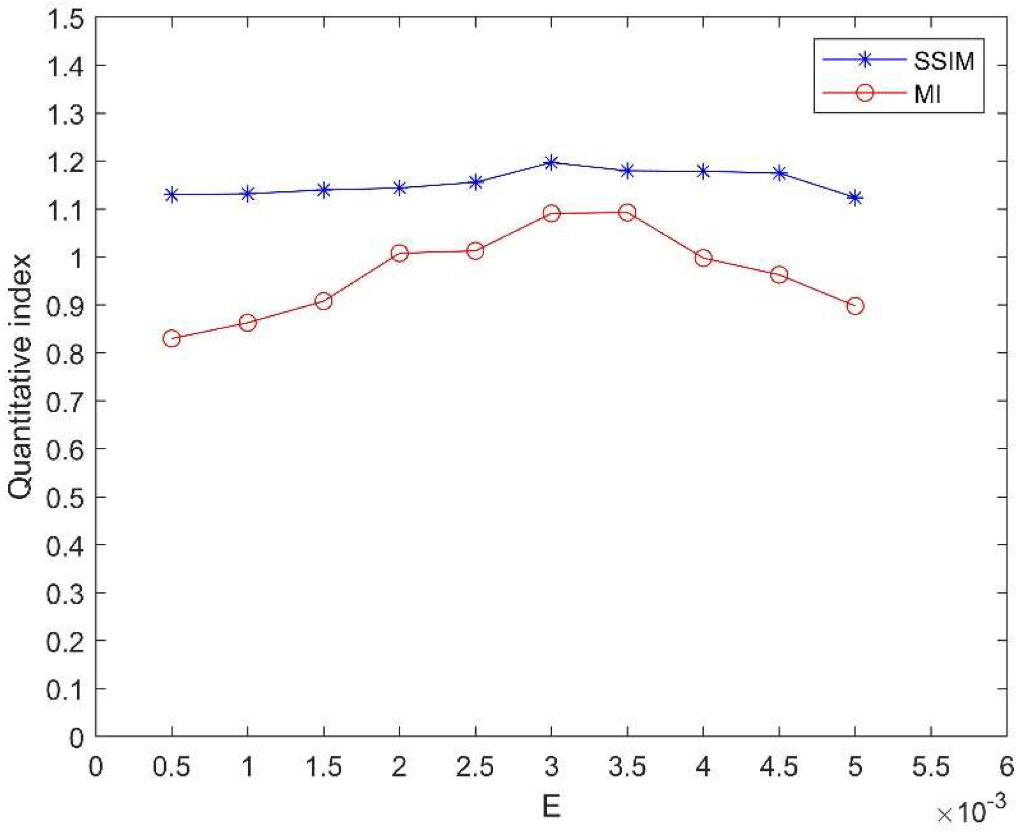
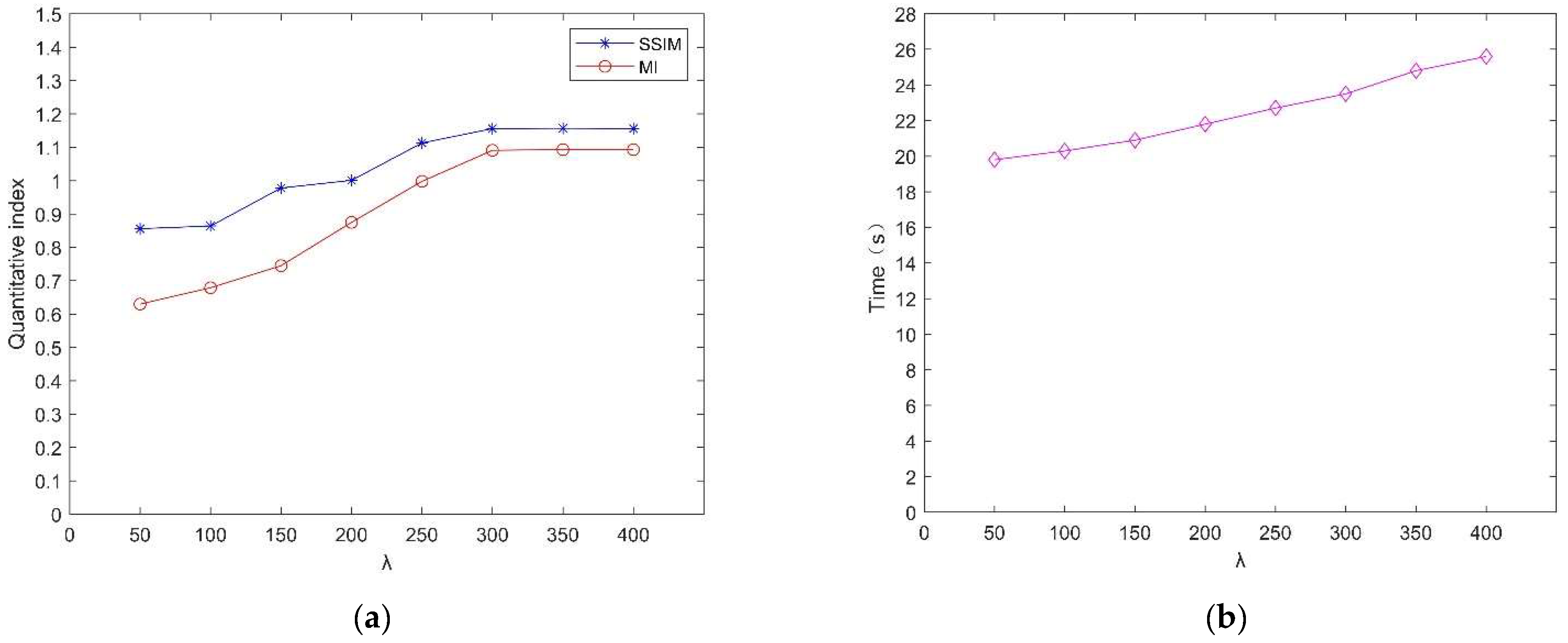
4.2. Parameter Settings

The controlled variable method is utilized to analyze the two free parameters in the model: the number of iterations λ in Equation (15) and the sparse reconstruction error parameter E in Equation (20). In addition, μ in Equation (15) is set to 10 8 , σ s in Equation (17) is set to 0.1, and parameter P in Equation (20) is set to 0.001.
  • The discussion of E
First, fix λ = 200 and then use the two indicators SSIM and MI to analyze the performance under different E . The experimental results are shown in the Figure 5. It can be seen that both indicators are better when E = 0.003 , and the fusion performance decreases when E < 0.003 or E > 0.003 . Therefore, after comprehensive consideration, the best value for E is 0.003.
  • The discussion of λ
If λ is too small, it will affect the denoising effect, but if λ is too large, it will affect the speed of the experiment. Therefore, it is very necessary to choose an appropriate number of iterations. Fix E = 0.003 . In order to better determine the number of iterations, SSIM, MI, and time T are used to observe the fusion performance and speed. It can be seen from Figure 6 that when λ < 300 , as the number of iterations increases, the image fusion effect gets better and better. When λ > 300 , the fusion effect hardly changes. In addition, the fusion speed gradually slows down with an increase in the number of iterations. Taking two factors into consideration, the best value for λ is 300.

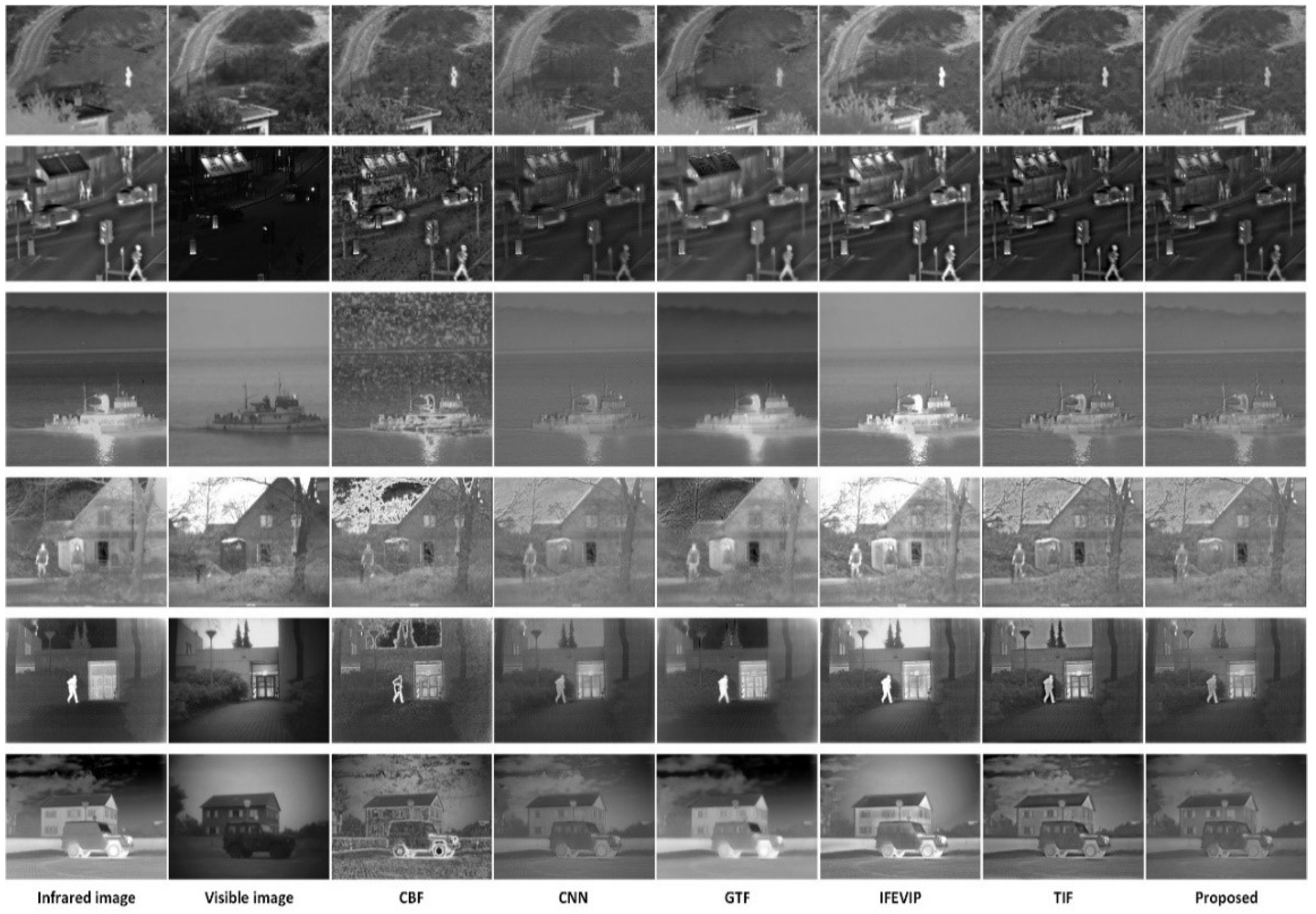
4.3. Noise-Free Image Fusion and Evaluation

Figure 7 shows the fusion results of the proposed algorithm and the comparison algorithm. The first column contains infrared images, and the second column contains visible images; the remaining images are the fusion images obtained by various methods.

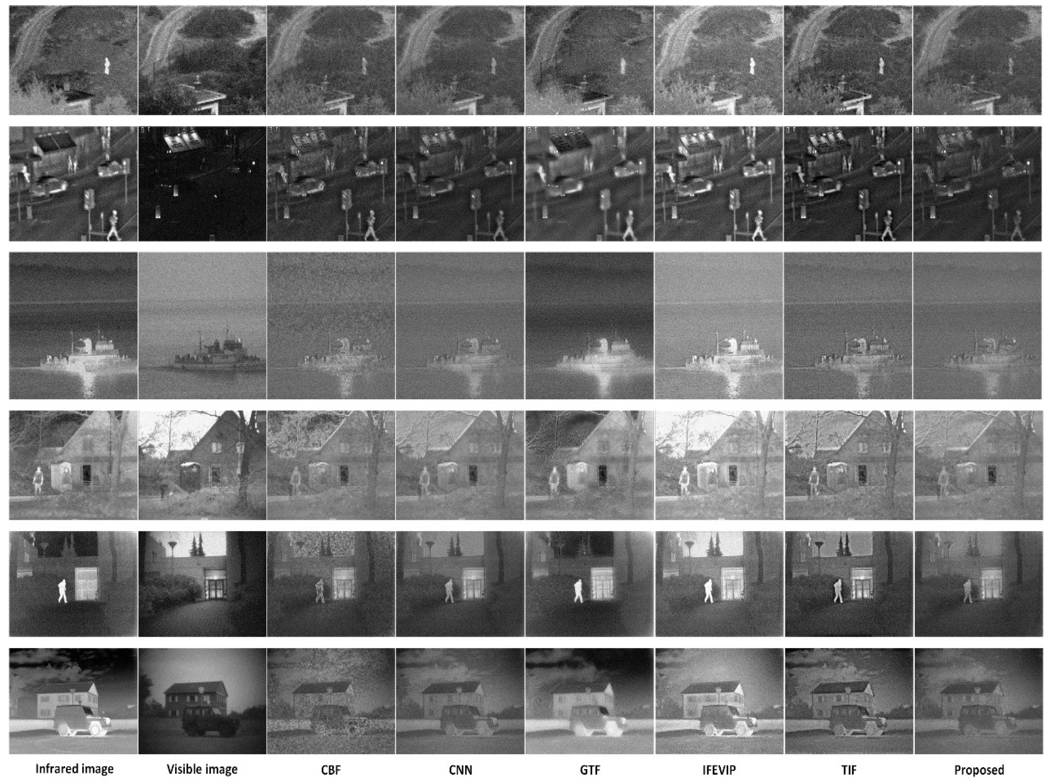
4.3.1. Subjective Evaluation

It can be seen from Figure 7 that the proposed method can retain more detail information, and there is less manual information. This is because the proposed two-scale decomposition algorithm can well separate the noise information and other main detail information, and the fusion rules are set appropriately. However, the salient features of the images obtained by CBF are not obvious and contain more artificial noise information. Although the fusion images generated by the CNN have lower brightness than the images generated by the proposed algorithm, the structures are better preserved. The GTF and IFEVIP methods maintain a good brightness, but the visual effects are too strengthened, resulting in obvious errors in the results. The TIF method has the phenomenon of fuzzy internal characteristics. Therefore, in the fusion results, the proposed algorithm can preserve the important content of the source image and obtain the best visual performance in terms of brightness and structural details, which means that the proposed algorithm can produce better subjective performance.

4.3.2. Objective Evaluation

Figure 8 shows the different objective evaluation values of the fusion results in the six pairs of images. From each subgraph in Figure 8, we can see that the index values of the proposed algorithm are almost all the highest, especially for the four indexes of Q A B / F , Q C B , MI, and PSNR; the proposed algorithm is always better compared to other algorithms. For the EN indicator, the proposed algorithm only performs poorly in the boat image. In addition, compared with other algorithms, the proposed algorithm has obvious advantages in the Q A B / F index, and the value in Figure 8 is significantly higher than other methods. Among various evaluation indicators, the proposed algorithm is not optimal in only a few places, but it can still be proven that the proposed algorithm has good performance.
In summary, the proposed algorithm performs well both qualitatively and quantitatively for the fusion of noise-free infrared and visible images.

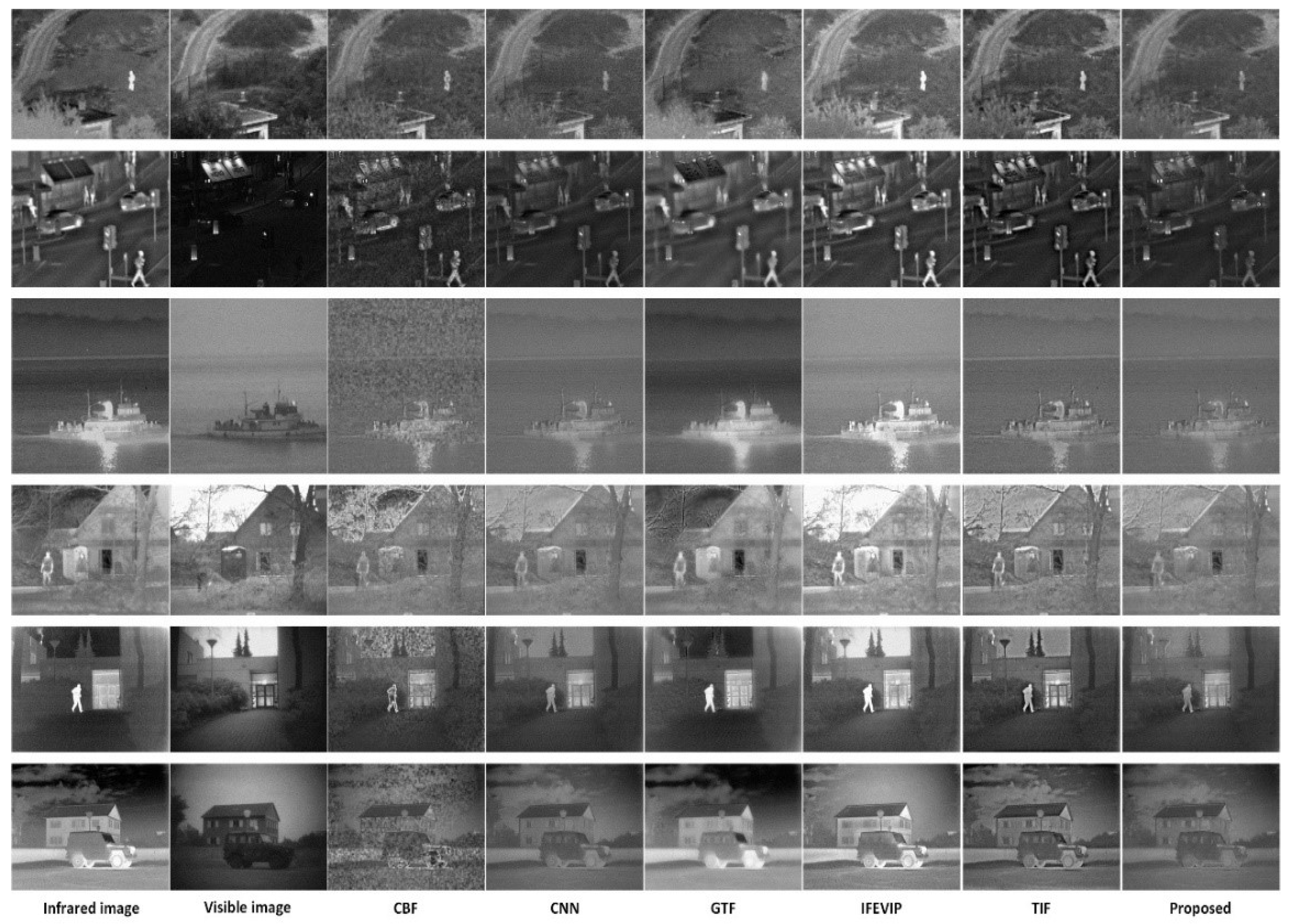
4.4. Noisy Image Fusion and Evaluation

Figure 9 and Figure 10 are examples of six pairs of noisy infrared and visible images. The noise intensity of the source images in Figure 9 and Figure 10 are 10 and 20, respectively. The first column of Figure 9 and Figure 10 contains the infrared images, and the second column contains the visible images; the remaining images are the fusion images obtained by various methods.

4.4.1. Subjective Evaluation

When the noise intensity is 10, the noise-removing capabilities of CBF and TIF methods are insufficient, and their fusion results lack useful information. The CNN method has a certain denoising effect, but the result is too low in contrast. GTF and IFEVIP methods can denoise effectively to a certain extent, but the contrast is too high and the image is unnatural. These two methods can be fused in a noisy environment, but some irrelevant information will be introduced, resulting in unreal visual effects. Compared with other algorithms, the proposed algorithm has the best fusion performance in detail reservation, and the noise in the fusion results is significantly reduced simultaneously, so it has good performance in denoising.
When the noise intensity reaches 20, the contours of the fusion results obtained by the CBF, CNN, and TIF methods have been severely damaged, and a large number of outstanding mistakes have been taken into the fusion results. In the IFEVIP method, the contrast is too high. Although the GTF method can denoise, the result is too smooth and lacks detail information. In contrast, the fusion results of the proposed algorithm not only preserve the detail content, contrast, and structure preservation of the source image, but its denoising effect is also remarkable.

4.4.2. Objective Evaluation

The objective evaluation of fusion results is shown in Table 1 and Table 2. Compared with CBF, CNN, GTF, IFEVIP, and TIF methods, the proposed method can obtain better objective analysis results, and is basically consistent with the objective evaluation results of noise-free image fusion. So, it proves the usefulness and superiority of the method proposed in this paper.
In summary, for the fusion of noisy infrared and visible images, the proposed algorithm has a good performance both qualitatively and quantitatively. This is because the two-scale decomposition algorithm designed in this paper can well separate the noise information and structural information in the source image, which are reflected in the high-frequency layer and the low-frequency layer, respectively. Through the adaptive sparse fusion algorithm, the denoising fusion of the high-frequency layer can be adaptively realized according to the intensity of the noise, and there will be no phenomenon of excessive denoising or insufficient denoising, which lays the foundation for the final fusion effect.

4.5. Computational Efficiency

In order to test the real-time performance of the algorithm in this paper, the various methods were placed in the same experimental environment for comparison, and the average execution time comparison is shown in Table 3. Since the experiment needs to perform multiple iterations and achieve partial fusion through sparse representation, the efficiency of the proposed method is not very high. Therefore, in future research, improving algorithm performance and increasing computational efficiency are important research directions.

5. Conclusions

In this paper, an infrared and visible image fusion algorithm based on optimized low-rank matrix decomposition and guided filtering is proposed. The proposed algorithm takes advantage of the filtering effect of low-rank matrix decomposition on noisy images, and introduces a reconstruction factor to minimize the error to improve the decomposition efficiency and performance. The final two-scale decomposition is achieved through guided filtering, and the noise information and structure information are better separated to obtain a better fusion performance. A large number of fusion results show that the proposed algorithm is obviously superior to the existing fusion methods in visual and quantitative evaluation, and can obtain strong anti-noise performance. Furthermore, the method can be effectively extended to image fusion problems of other modalities.

Author Contributions

Methodology, Y.L.; software, J.Y.; validation, C.W.; investigation, Y.Z.; resources, Y.H.; data curation, Z.L.; writing—original draft preparation, J.J.; writing—review and editing, J.J., C.W., Y.Z, Y.L., Y.H., Z.L., J.Y. and F.H.; funding acquisition, F.H. All authors have read and agreed to the published version of the manuscript.

Funding

This research was funded by the National Natural Science Foundation of China, grant number 62171467, and the Natural Science Foundation of Hebei Province, grant number F2021506004.

Conflicts of Interest

The authors declare no conflict of interest.

References

  1. Hu, Y.; Xu, C.; Li, Z.; Lei, F.; Feng, B.; Chu, L.; Nie, C.; Wang, D. Detail enhancement multi-exposure image fusion based on homomorphic filtering. Electronics 2022, 11, 1211. [Google Scholar] [CrossRef]
  2. Su, Y.; Tang, C.; Li, B.; Qiu, Y.; Zheng, T.; Lei, Z. Greyscale image encoding and watermarking based on optical asymmetric cryptography and variational image decomposition. J. Mod. Opt. 2018, 66, 377–389. [Google Scholar] [CrossRef]
  3. Kowsher, M.; Alam, M.A.; Uddin, M.J.; Ahmed, F.; Ullah, M.W.; Islam, M.R. Detecting third umpire decisions & automated scoring system of cricket. In Proceedings of the 2019 International Conference on Computer, Communication, Chemical, Materials and Electronic Engineering (IC4ME2), Rajshahi, Bangladesh, 11–12 July 2019; pp. 1–8. [Google Scholar]
  4. Liu, Y.; Chen, X.; Cheng, J.; Peng, H.; Wang, Z. Infrared and visible image fusion with convolutional neural networks. Int. J. Wavelets Multiresolut. Inf. Process. 2018, 16, 1850018. [Google Scholar] [CrossRef]
  5. Liu, Y.; Chen, X.; Ward, R.K.; Wang, Z.J. Image fusion with convolutional sparse representation. IEEE Signal Process. Lett. 2016, 23, 1882–1886. [Google Scholar] [CrossRef]
  6. Luo, X.; Li, X.; Wang, P.; Qi, S.; Guan, J.; Zhang, Z. Infrared and visible image fusion based on NSCT and stacked sparse autoencoders. Multimed. Tools Appl. 2018, 77, 22407–22431. [Google Scholar] [CrossRef]
  7. Hui, L.; Wu, X.J.; Kittler, J. Infrared and visible image fusion using a deep learning framework. In Proceedings of the 2018 24th International Conference on Pattern Recognition (ICPR), Beijing, China, 20–24 August 2018. [Google Scholar]
  8. Cardone, D.; Spadolini, E.; Perpetuini, D.; Filippini, C.; Chiarelli, A.M.; Merla, A. Automated warping procedure for facial thermal imaging based on features identification in the visible domain. Infrared Phys. Technol. 2020, 112, 103595. [Google Scholar] [CrossRef]
  9. Singh, S.; Gyaourova, A.; Bebis, G.; Pavlidis, I. Infrared and visible image fusion for face recognition. Biometric Technology for Human Identification; SPIE: Reno, NV, USA, 2004; Volume 5404, pp. 585–597. [Google Scholar] [CrossRef]
  10. Wang, N.Y.; Wang, W.L.; Guo, X.R. A new image fusion method based on improved PCNN and multiscale decomposition. Adv. Mater. Res. 2014, 834–836, 1011–1015. [Google Scholar] [CrossRef]
  11. Zhu, J.; Jin, W.; Li, L.; Han, Z.; Wang, X. Multiscale infrared and visible image fusion using gradient domain guided image filtering. Infrared Phys. Technol. 2018, 89, 8–19. [Google Scholar] [CrossRef]
  12. Ma, J.; Zhou, Z.; Wang, B.; Zong, H. Infrared and visible image fusion based on visual saliency map and weighted least square optimization. Infrared Phys. Technol. 2017, 82, 8–17. [Google Scholar] [CrossRef]
  13. Zhang, P.; Yuan, Y.; Fei, C.; Pu, T.; Wang, S. Infrared and visible image fusion using co-occurrence filter. Infrared Phys. Technol. 2018, 93, 223–231. [Google Scholar] [CrossRef]
  14. Duan, C.; Wang, Z.; Xing, C.; Lu, S. Infrared and visible image fusion using multi-scale edge-preserving decomposition and multiple saliency features. Optik 2020, 228, 165775. [Google Scholar] [CrossRef]
  15. Candes, E.J.; Li, X.; Ma, Y.; Wright, J. Robust principal component analysis? arXiv 2009, arXiv:0912.3599. [Google Scholar] [CrossRef]
  16. Boyd, S.; Parikh, N.; Chu, E.; Peleato, B.; Eckstein, J. Distributed optimization and statistical learning via the alternating direction method of multipliers. Found. Trends Mach. Learn. 2011, 3, 1–122. [Google Scholar] [CrossRef]
  17. Jiang, Y.; Wang, M. Image fusion using multiscale edge-preserving decomposition based on weighted least squares filter. IET Image Process. 2014, 8, 183–190. [Google Scholar] [CrossRef]
  18. Salehi, H. Image de-speckling based on the coefficient of variation, improved guided filter, and fast bilateral filter. Int. J. Image Graph. 2021, 21, 2250036. [Google Scholar] [CrossRef]
  19. Li, S.; Kang, X.; Hu, J. Image fusion with guided filtering. IEEE Trans. Image Process. 2013, 22, 2864–2875. [Google Scholar]
  20. Aharon, M.; Elad, M.; Bruckstein, A. K-SVD: An algorithm for designing overcomplete dictionaries for sparse representation. IEEE Trans. Signal Process. 2006, 54, 4311–4322. [Google Scholar] [CrossRef]
  21. Donoho, D.L.; Tsaig, Y.; Drori, I.; Starck, J.L. Sparse solution of underdetermined systems of linear equations by stagewise orthogonal matching pursuit. IEEE Trans. Inf. Theory 2012, 58, 1094–1121. [Google Scholar] [CrossRef]
  22. Yang, F.; Li, J.; Xu, S.H.; Pan, G.F. The research of a video segmentation algorithm based on image fusion in the wavelet domain. In Proceedings of the 5th International Symposium on Advanced Optical Manufacturing and Testing Technologies: Smart Structures and Materials in Manufacturing and Testing, Dalian, China, 26–29 April 2010; Volume 7659, pp. 279–285. [Google Scholar]
  23. Shreyamsha Kumar, B.K. Image fusion based on pixel significance using cross bilateral filter. Signal Image Video Process. 2015, 9, 1193–1204. [Google Scholar] [CrossRef]
  24. Ma, J.; Chen, C.; Li, C.; Huang, J. Infrared and visible image fusion via gradient transfer and total variation minimization. Inf. Fusion 2016, 31, 100–109. [Google Scholar] [CrossRef]
  25. Zhang, Y.; Zhang, L.; Bai, X.; Zhang, L. Infrared and visual image fusion through infrared feature extraction and visual information preservation. Infrared Phys. Technol. 2017, 83, 227–237. [Google Scholar] [CrossRef]
  26. Bavirisetti, D.P.; Dhuli, R. Two-scale image fusion of visible and infrared images using saliency detection. Infrared Phys. Technol. 2016, 76, 52–64. [Google Scholar] [CrossRef]
  27. Chibani, Y. Additive integration of SAR features into multispectral SPOT images by means of the à trous wavelet decomposition. ISPRS J. Photogramm. Remote Sens. 2006, 60, 306–314. [Google Scholar] [CrossRef]
  28. Xydeas, C.S.; Pv, V. Objective image fusion performance measure. Electron. Lett. 2000, 56, 181–193. [Google Scholar] [CrossRef] [Green Version]
  29. Chen, Y.; Blum, R.S. A new automated quality assessment algorithm for night vision image fusion. In Proceedings of the 2007 41st Annual Conference on Information Sciences and Systems, Baltimore, MD, USA, 14–16 March 2007; pp. 518–523. [Google Scholar]
  30. Qu, G.; Zhang, D.; Yan, P. Information measure for performance of image fusion. Electron. Lett. 2002, 38, 313–315. [Google Scholar] [CrossRef] [Green Version]
  31. Wang, Z.; Bovik, A.C.; Sheikh, H.R.; Simoncelli, E.P. Image quality assessment: From error visibility to structural similarity. IEEE Trans. Image Process. 2004, 13, 600–612. [Google Scholar] [CrossRef] [Green Version]
  32. Jagalingam, P.; Hegde, A.V. A Review of Quality Metrics for Fused Image. Aquat. Procedia 2015, 4, 133–142. [Google Scholar] [CrossRef]
Figure 1. The principle diagram of guided filtering.
Electronics 11 02003 g001
Figure 2. The framework of the fusion algorithm.
Electronics 11 02003 g002
Figure 3. Two-scale decomposition image.
Electronics 11 02003 g003
Figure 4. Six pairs of source images.
Electronics 11 02003 g004
Figure 5. Quantitative evaluation of the fused images produced by different E .
Electronics 11 02003 g005
Figure 6. Quantitative evaluation of the fused images produced by different λ . ((a) represents the quality evaluation value of different λ , and (b) represents the consumption time of different λ .)
Electronics 11 02003 g006
Figure 7. Fusion results of noise-free images.
Electronics 11 02003 g007
Figure 8. Objective evaluation metrics for fusion results.
Electronics 11 02003 g008
Figure 9. Fusion results of noisy images ( σ = 10 ).
Electronics 11 02003 g009
Figure 10. Fusion results of noisy images ( σ = 20 ).
Electronics 11 02003 g010
Table 1. Quantitative index of image fusion results ( σ = 10 ).
Source ImagesIndexCBFCNNGTFIFEVIPTIFProposed
CampEN6.6016.7616.8206.9016.4036.797
Q A B F 0.3170.4220.4590.3800.3590.480
Q C B 0.5170.5500.4750.5200.5610.568
MI0.8890.9050.9330.7860.9451.080
SSIM 1.2131.1091.0901.2241.2001.297
PSNR 58.46758.54857.78256.80758.36258.933
ShopEN6.5596.8076.7396.8836.6086.890
Q A B F 0.3010.4530.4080.4740.4080.497
Q C B 0.4470.4380.2940.3840.4460.472
MI0.8181.2250.8781.4791.0501.595
SSIM 0.9801.0500.7641.1201.0181.194
PSNR 59.63759.88959.22259.17759.71259.997
BoatEN6.1416.7566.7886.2836.6086.867
Q A B F 0.2730.4810.4750.4710.3170.496
Q C B 0.4390.5690.4690.4880.5470.576
MI0.4740.7711.3151.3810.5401.378
SSIM 1.1451.2001.0951.2171.2291.295
PSNR 59.67459.83359.15958.14859.80459.826
HouseEN6.7836.6406.5126.9896.8717.142
Q A B F 0.3050.4530.4560.3940.3680.456
Q C B 0.4740.4740.4700.5080.5680.574
MI0.7270.8961.0271.5350.7911.696
SSIM 1.1281.1731.1001.2241.2021.293
PSNR 59.72060.17259.45858.56060.06860.198
BuildingEN6.9356.8827.1147.2727.0317.349
Q A B F 0.2780.4760.4400.4070.3410.540
Q C B 0.4670.4850.4350.5090.5320.556
MI0.8071.0361.1691.1400.9651.182
SSIM 1.1171.1310.9911.2131.1591.294
PSNR 59.17559.34958.73658.00459.23559.943
CarEN6.7876.6277.1137.1446.9067.506
Q A B F 0.2300.4210.4120.4550.3510.527
Q C B 0.4140,3740.3660.4240.4680.476
MI0.4210.6720.8440.6710.7260.926
SSIM 0.9411.0300.8781.1381.0621.189
PSNR 58.13158.37157.87557.13758.31558.494
Table 2. Quantitative index of image fusion results ( σ = 20 ).
Source ImagesIndexCBFCNNGTFIFEVIPTIFProposed
CampEN6.9426.8907.1317.2647.1237.277
Q A B F 0.2850.3220.4960.3430.3110.429
Q C B 0.4740.4560.4980.4920.5520.553
MI0.8700.8630.7111.0080.9261.091
SSIM 1.1601.1320.9481.1441.0701.197
PSNR 57.92657.99556.99255.80157.67158.291
ShopEN6.8786.9726.9837.2376.8817.519
Q A B F 0.3260.3250.4070.4490.3380.520
Q C B 0.4410.4260.3020.4720.4670.495
MI0.9600.7480.7001.5100.8661.330
SSIM 1.0090.8540.6151.0630.9241.094
PSNR 59.59359.64558.74258.78259.50859.928
BoatEN6.6126.7646.2256.8556.6536.995
Q A B F 0.2680.3840.5150.3320.2830.521
Q C B 0.4850.4930.4870.5010.5240.542
MI0.4520.5500.9570.8310.4610.977
SSIM 1.1361.0630.9101.1281.0641.195
PSNR 59.32459.32258.36257.56659.26759.689
HouseEN6.9106.9257.3147.2117.1297.494
Q A B F 0.2760.3460.4210.3480.3090.481
Q C B 0.4710.4480.4870.5000.4240.551
MI0.4920.6030.5680.4250.5850.649
SSIM 1.1281.1000.9451.1471.0641.193
PSNR 59.68059.08358.97558.18859.78759.928
BuildingEN7.1527.1507.3397.5457.3007.062
Q A B F 0.2670.3250.4760.3560.3030.486
Q C B 0.4640.4420.4490.4690.5190.538
MI0.7350.8800.7110.8670.7860.965
SSIM 1.0881.0630.8401.1371.0271.193
PSNR 58.97859.06658.12157.50158.90459.885
CarEN6.9276.8977.7557.3627.1077.780
Q A B F 0.2520.3420.4580.4050.3000.535
Q C B 0.4310.3870.3750.4280.4640.493
MI0.4160.5001.1751.1180.5421.342
SSIM 1.0080.9830.7181.0780.9531.089
PSNR 58.04858.19757.37856.82758.10858.435
Table 3. Computational efficiency of different methods.
MethodCBFCNNGTFIFEVIPTIFProposed
Time/s10.7323.162.911.341.0322.03
Publisher’s Note: MDPI stays neutral with regard to jurisdictional claims in published maps and institutional affiliations.

