A Practical Guide to Estimating Coil Inductance for Magnetic Resonance Applications

Abstract

Radiofrequency (RF) coils are employed to transmit and/or receive signals in Magnetic Resonance (MR) systems. The design of home-made, organ-specific RF coils with optimized homogeneity and/or Signal-to-Noise Ratio (SNR) can be a plus in many research projects. The first step requires accurate inductance calculation, this depending on the conductor’s geometry, to later define the tuning capacitor necessary to obtain the desired resonance frequency. To fulfil such a need it is very useful to perform a priori inductance estimation rather than relying on the time-consuming trial-and-error approach. This paper describes and compares two different procedures for coil inductance estimation to allow for a fast coil-prototyping process. The first method, based on calculations in the quasi-static approximation, permits an investigation on how the cross-sectional geometry of the RF coil conductors affects the total inductance and can be easily computed for a wide variety of coil geometries. The second approach uses a numerical full-wave method based on the Finite-Difference Time-Domain (FDTD) algorithm, and permits the simulation of RF coils with any complex geometry, including the case of multi-element phased array. Comparison with workbench measurements validates both the analytical and numerical results for RF coils operating within a wide field range (0.18–7 T).

1. Introduction

Magnetic Resonance Imaging (MRI) and Magnetic Resonance Spectroscopy (MRS) are non-ionizing and non-invasive diagnostic techniques based on the Nuclear Magnetic Resonance (NMR) phenomenon. In both techniques, the design of the radiofrequency (RF) coils is a fundamental issue that implicate image quality of specific organs/tissues [1].

RF coils can be categorized into two groups accordingly to their shape: volume coils, such as the birdcage and solenoid, able to generate a uniform field in a large cylindrical volume surrounding the sample and employed for transmission and/or reception phases; and surface coils, constituting loops of various shapes, which guarantee high sensitivity in the nearby tissue and are mainly employed as receive-only coils due to their relatively poor magnetic field homogeneity [2,3].

Phased-array RF coils [4] are another technical option, able to provide a large sensitivity region like that of the volume coils, and a high Signal-to-Noise Ratio (SNR), as provided by surface RF coils, with the great potential of accelerated image acquisition and reduced scan time [5].

From a practical point of view, RF coils realized in a Do-It-Yourself approach are generally built using two different cross-sectional geometry conductors, i.e., circular wire and flat strip (hereafter named “wire” and “strip”, respectively). To design application-optimized RF coils, an accurate simulation process is necessary. The design process must allow for the choice of coil parameters (sizes and conductor geometry), ensuring the optimal balance among magnetic RF field distribution and SNR. Although a complete RF coil design includes the computation of the loaded RF coil magnetic field pattern and the total losses (coil resistance and sample-induced resistance), the first design step can be performed with a priori inductance estimation, useful for avoiding trial-and-error methods in the RF coil-tuning process. One of the earliest expressions for analytic inductance calculation, providing simple formulae for calculating the inductance of RF coils, was given by Wheeler in 1928 [6]. Earlier reference textbooks about the procedure of analytic inductance calculation suitable for a large variety of RF coils were given by Terman [7] and Grover [8], where a collection of tables and methods were presented. The subject has subsequently been developed, building upon the previous work, reformulating equations for the specific field of applications [3,9].

Over the past 30 years, a large number of RF coil geometries have been used for MRI applications, ranging from ultra-low (µT) to ultra-high (T) magnetic fields, and from ultra-small (micron) to very large (1 m) sizes. The first step in designing the RF coil is to evaluate the self-inductance, a parameter necessary for selecting the correct tuning capacitor, i.e., the Larmor frequency that depends on the operating static magnetic field B₀ and the nuclei of interest. Although textbooks and hundreds of papers are available for the practical calculation of specific RF coil inductances [1,2,3], no comprehensive work is available with practical guides that allows for the accurate estimation of coil inductance for the most commonly used geometries (volume, surface, phased array) suitable for MRI applications. Such a priori inductance estimation tool would make the RF coil implementation process quite fast, avoiding the time-consuming and expensive trial-and-error approach. Moreover, most of the literature formulations for RF coil inductance estimation do not take into account the exact conductor geometry [2,4,8,10] and/or perform numerical calculation by making approximations, affecting the inductance accuracy [11,12].

The present work describes and compares two procedures for RF coils’ inductance estimation to allow for a fast RF coil-prototyping process. The first method, based on analytical calculation, can be easily numerically implemented, and allows for extremely fast implementation (of the order of seconds on a modern laptop) for simple-geometry RF coils. The second requires the use of an electromagnetic solver which implements the Finite-Difference Time-Domain (FDTD) algorithm; it requires longer calculation times (of the order of hours) and it allows for simulation of RF coils with any complex geometry, including the case of multi-element phased array. The first approach is particularly suitable for exploring large portions of coils’ parameter space for fast optimization, and the second is more appropriate for parameters’ fine-tuning. Results provided by both approaches are compared with workbench results obtained on different RF coil prototypes to provide useful insights for a fast and effective prototyping. The presented RF coils are suitable for ¹H and ¹³C operating within a wide magnetic field range (0.2–7 T).

2. Inductance Estimation Methods

2.1. Analytical Calculation

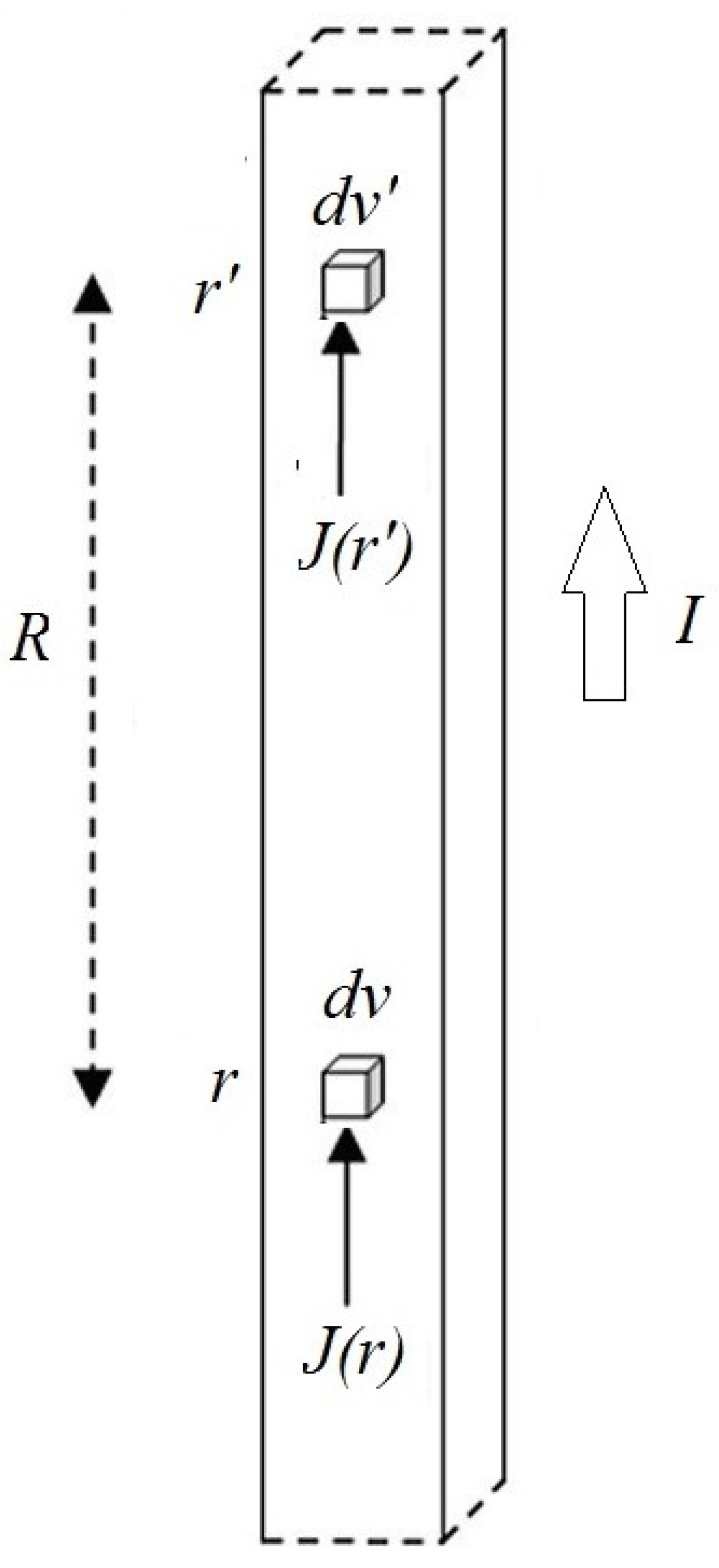
The inductance of a conductor can be calculated, in the quasi-static approximation, by using the following expression [2]:

$$L=\frac{{\mu }_0}{4\pi I^2}{{\displaystyle \iiint }}_V{{\displaystyle \iiint }}_V\frac{J\left(r\right)\cdot J\left(r^{\prime }\right)}{R}dvd{v}^{\prime }$$

(1)

where J is the current density in the conductor, μ₀ is the permeability of free space, I represents the total current in the conductor, V is the conductor volume, and $R=\left|r-r^{\prime }\right|$ (Figure 1).

Such a quasi-static approach is applicable for RF coils with a length that is a small fraction (<1/10) of the Larmor wavelength associated with the B₀ static field [2], and it has been demonstrated to be useful for the design of RF coils constituting linear and/or circular conductor segments (birdcages [13], solenoids [14], circular and square loops [15], butterfly coils [16]). In this work, Equation (1) has been applied for various-geometry RF coils’ inductance calculation considering different conductor sizes and typology (strip and wire). Such RF coil inductance calculations were performed by custom-made routines written with IDL 6.0 (Interactive Data Language, Visual Information Solutions, Boulder, CO, USA).

2.2. FDTD Method

The FDTD method, introduced for the first time by Yee [17], solves Maxwell’s equations in the time domain using a discretization of the temporal and spatial parameters with the finite difference approximation. FDTD does not require the solving of any matrix equations, and it has been widely used in the context of MRI applications for numerical simulations of electromagnetic fields interaction with the human body and/or phantoms. For example, Amjad [18] performed calculation of the power deposition inside a phantom for estimating RF-induced temperature rise. Wang [19] employed the FDTD algorithm for specific absorption rate (SAR) and temperature calculations for the human head in a volume RF coil at different frequencies. Chen [20] estimated SAR and B₁ field inside the human head generated by a shielded birdcage RF coil. In another paper [21], FDTD was employed for the estimation of the average and peak SAR values on human thorax models with different masses and sizes. Giovannetti [22] proposed an FDTD-based RF coil model able to supply sample-induced resistance and magnetic field pattern calculation, without approximations in sample and coil geometries. A very recent paper by Giovannetti et al. [23] investigated the FDTD accuracy for separately estimating RF coil conductor and radiative loss contributions, comparing the results with the Finite Element Method (FEM) analysis and validating the results with workbench measurements performed on a home-built RF coil. In this work, numerical simulations were performed with the FDTD method using the commercially available software XFdtd (Remcom, State College, PA, USA), which allows for the simulation of RF coils with arbitrary geometries. For inductance evaluation, the simulated RF coils constituted a Perfect Electric Conductor (PEC) with wire or strip section; moreover, an adaptive non-uniform mesh (finer in the coil conductor area) was employed to minimize the computational load and time while achieving a good degree of accuracy. The FDTD inductance estimation was performed with the following two approaches.

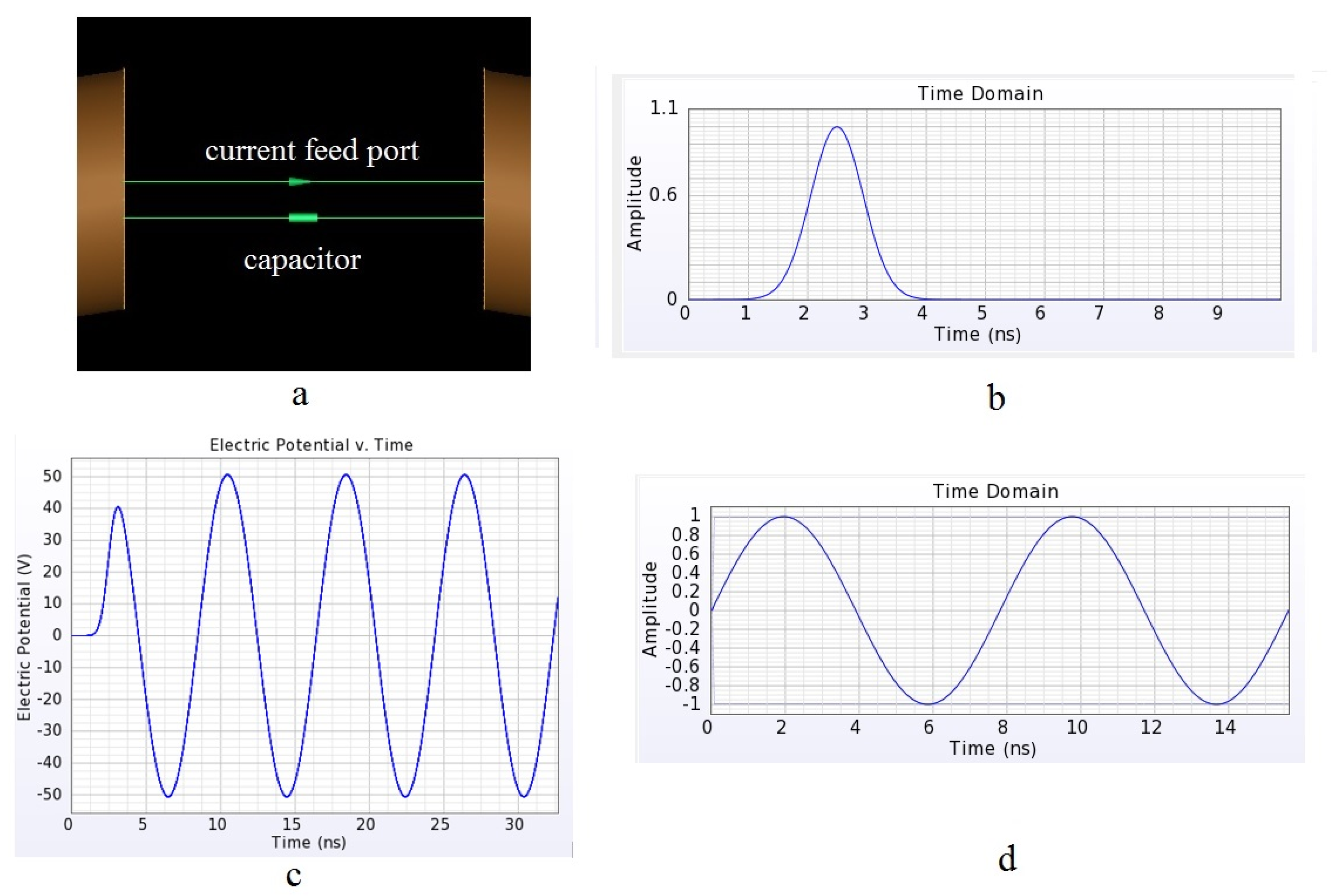
In the first approach (Method A), a lossless tuning capacitor and an ideal current feed port were inserted in the RF coil (Figure 2a). A Gaussian broadband pulse excitation in the feed port (Figure 2b) induces a damped voltage oscillation on the capacitor (Figure 2c), and such behaviour allows for the determination of the resonance frequency and RF coil inductance. In the second approach (Method B), a 50 Ω port feed with sinusoidal current of frequency equal to the Larmor frequency (Figure 2d) was used, and the inductance of the purely inductive coil was estimated from direct impedance calculation. Perfect Matched Layer (PML) boundary conditions were employed in both methods to avoid wave reflections from the boundary of the computational domain.

3. Design and Simulation of RF Coils

3.1. Volume RF Coils

3.1.1. Birdcage

The birdcage is the workhorse volume RF coil in many MRI preclinical and clinical applications from the very low field (mT) up to ultra-high field (7 T) [24,25]. The implementation of double-tuned RF coils based on the birdcage design has been also reported [26,27,28,29].

The birdcage coil is relatively easy to manufacture and, depending on its size, can successfully be applied from the low-field to the ultra-high-field regime. The inductance of the birdcage RF coil with a circular section was analytically estimated by considering the “global” inductance of the N legs coil [25], defined by L_GLOB = Z_in/j2πf, where Z_in is the input impedance calculated at frequency f by using the transmission line approach [30]:

$$Z_{in}=Z_c\frac{sinh\left(N\lambda /2\right)}{2\cdot sinh\left(\lambda /2\right)sinh\left[\left(N-1\right)\cdot \left(\lambda /2\right)\right]}$$

(2)

where:

$$Z_c=\sqrt{\left[{\left(\frac{Z_1}{2}\right)}^2+Z_1{Z}_2\right]}$$

(3)

$$\lambda =arcosh\left(1+\frac{Z_1}{2Z_2}\right)$$

(4)

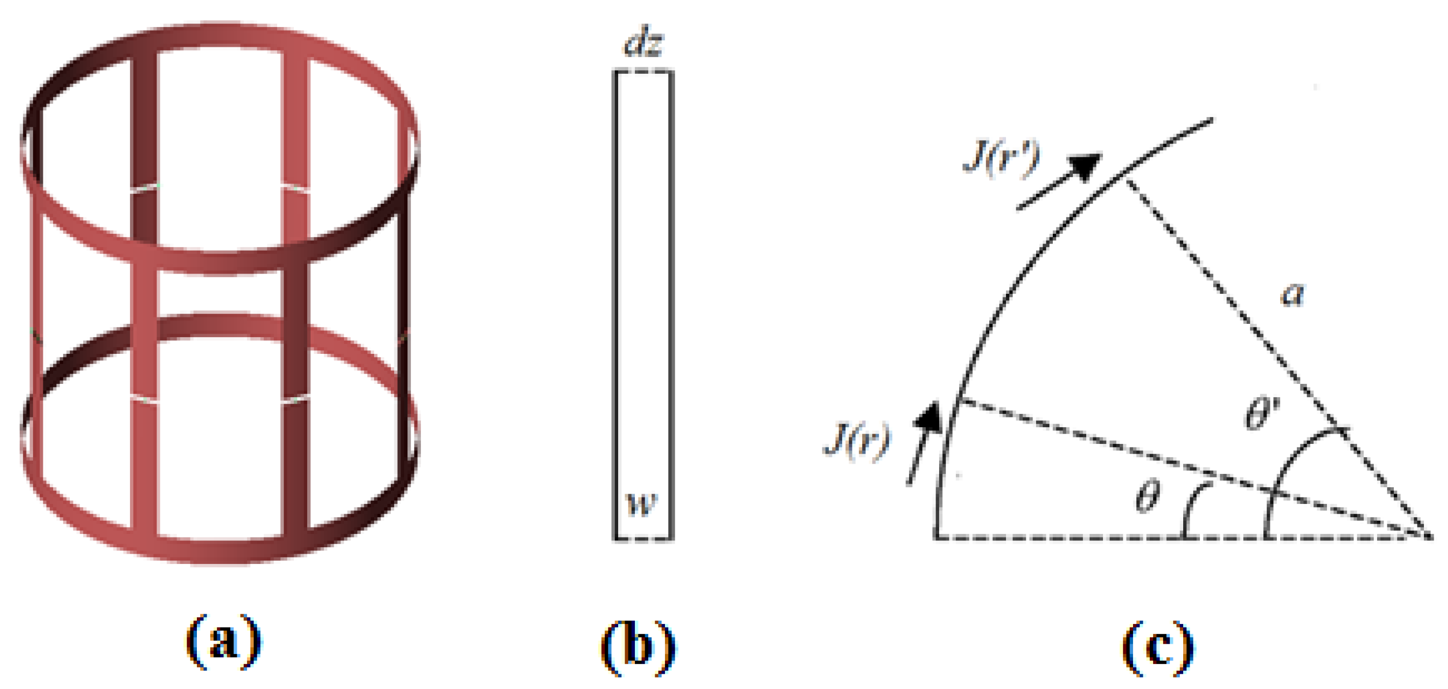
Z₁ and Z₂ represent the end-ring (inductance L_ER) and leg (inductance L_LEG) conductor impedances, respectively, which can be estimated by software implementing Equation (1) [13]. In particular, the inductance of the birdcage legs, constituting strip conductors with width w and length l, can be written as [13]:

$$L_{LEG}=\frac{{\mu }_{0}l}{2\pi }\left(ln\frac{2l}{w}+\frac{1}{2}\right)$$

(5)

while the end-rings’ strip segment inductance can be written according to the following expression [13]:

$$L_{ER}=\frac{{\mu }_0}{4\pi w^2}{{\displaystyle \int }}_{-\mathrm{w}/2}^{\mathrm{w}/2}{{\displaystyle \int }}_0^{2\pi /N}{{\displaystyle \int }}_{-\mathrm{w}/2}^{\mathrm{w}/2}{{\displaystyle \int }}_0^{2\pi /N}\frac{\mathit{cos}\left({\theta }^{\prime }-\theta \right)a^2}{R_1}d\theta dzd{\theta }^{\prime }d{z}^{\prime }$$

(6)

where a is the birdcage radius and

$$R_1=\sqrt{{\left[acos\theta -acos{\theta }^{\prime }\right]}^2+{\left[asin\theta -asin{\theta }^{\prime }\right]}^2+{\left(z-z^{\prime }\right)}^2}$$

(7)

Such calculations were performed by considering perfect conductor strips of negligible thickness. Figure 3a shows the birdcage FDTD CAD model, while Figure 3b,c show the lateral and upper side segment view of the birdcage end-rings, respectively.

To validate the computer implementation of the above formulas, we studied a birdcage RF coil. The presence of the RF shield was not considered, such us to calculate the “intrinsic” inductance of the birdcage. Coil #1 was an 8-leg lowpass birdcage tuned (C_T = 2 nF) at a frequency of about 8 MHz (¹H, 0.18 T) with length 11 cm, diameter 13.4 cm, and all segments realized by a 1 cm-width strip copper conductor with 35 μm thickness. This lowpass birdcage design is suitable as a receiver RF coil for a vertical B₀ MRI system (Esaote E-Scan 0.18 T) [13]. Such a prototype of a birdcage RF coil matching the above geometry was built and tuned with non-magnetic, high-quality capacitors (ATC-American Technical Ceramics, Fountain, SC, USA) connected at the center of each leg.

3.1.2. Solenoid

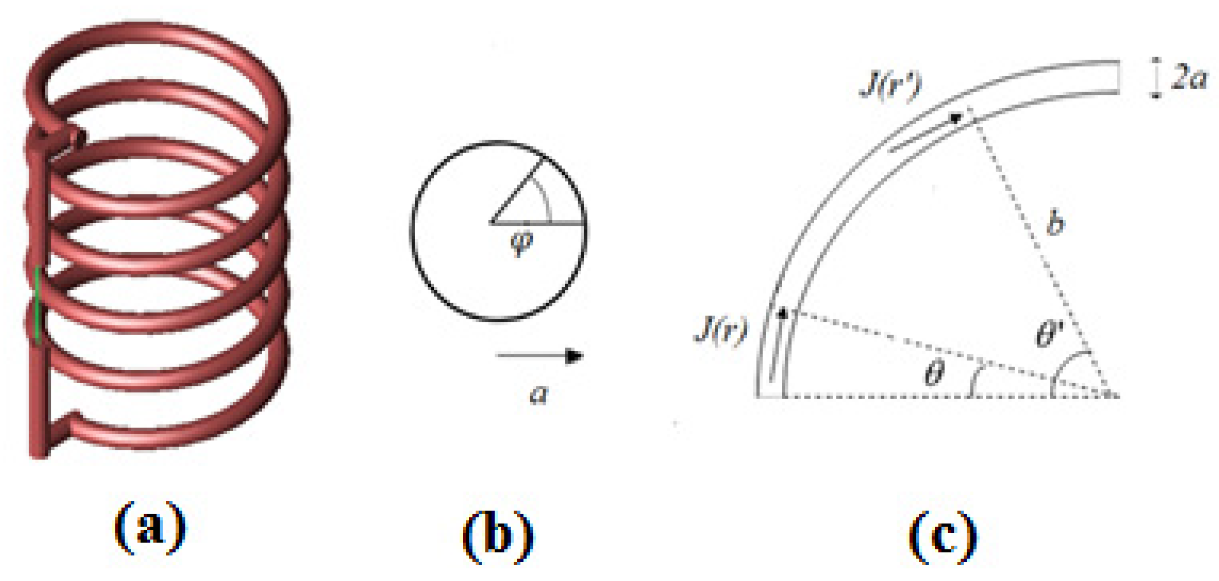
The solenoid RF coil has the advantage of high efficiency [31], but due to the axial orientation of the RF field and the relevant length of the conductor, it is more commonly adopted in low-to-medium field MRI systems with non-axial B₀ (i.e., C-shaped magnets) or in NMR instruments. The solenoid inductance (radius b and length h, constituted by N turns with wire of radius a) may be calculated with the following expression [14]:

$$L_{SOL-wire}=\frac{{\mu }_0}{4\pi {\left(2\pi a\right)}^2}{{\displaystyle \int }}_0^{2\pi }{{\displaystyle \int }}_0^{2\pi N}{{\displaystyle \int }}_0^{2\pi }{{\displaystyle \int }}_0^{2\pi N}\frac{cos\left({\theta }^{\prime }-\theta \right)a^2}{R_2}\left(b+acos\phi \right)\left(b+acos{\phi }^{\prime }\right)d\phi d\theta d{\phi }^{\prime }d{\theta }^{\prime }$$

(8)

where:

$$\begin{gathered} R_2={\left[{\left(bsin\theta +acos\phi sin\theta -bsin{\theta }^{\prime }-acos{\phi }^{\prime }sin{\theta }^{\prime }\right)}^2+{\left(asin\phi +k\theta -asin{\phi }^{\prime }-k{\theta }^{\prime }\right)}^2+ \\ {\left(bcos\theta +acos\phi cos\theta -bcos{\theta }^{\prime }-acos{\phi }^{\prime }cos{\theta }^{\prime }\right)}^2\right]}^{1/2} \end{gathered}$$

(9)

with $k=\frac{h}{\left(2N\pi \right)}$.

Figure 4a depicts the CAD solenoid model for FDTD simulations, while Figure 4b,c show the conductor section and the upper side view of a solenoid segment, respectively. To validate the implementation of the above expressions, we considered the design of a solenoid suitable for solid-state ¹H NMR operating at 300 MHz, hereafter called Coil #2, with the following geometry: 5.15 mm radius, 14.40 mm length, 0.912 mm wire radius, 5 turns [10].

3.2. Surface RF Coils

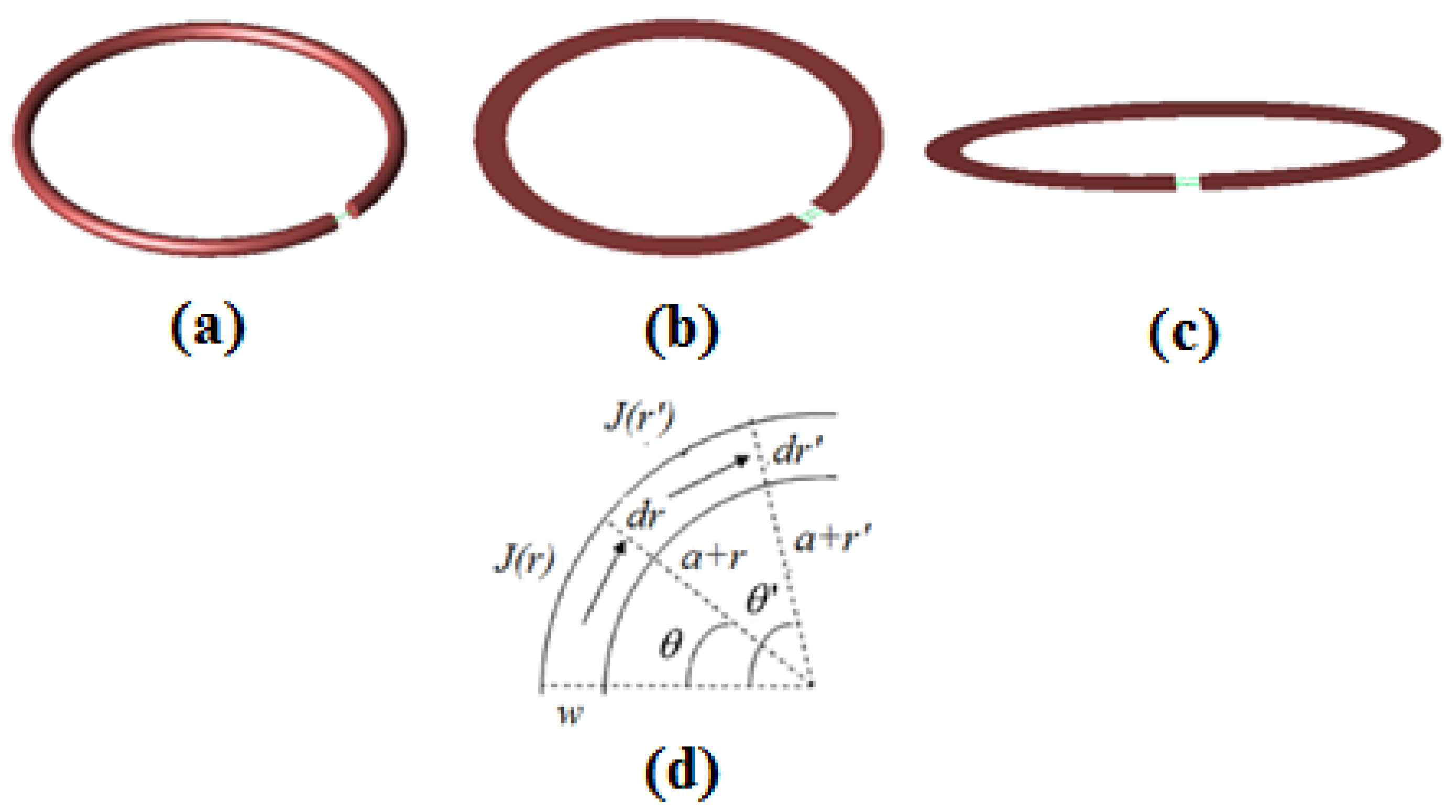
3.2.1. Circular Coil

The circular RF coil is an efficient option when signal homogeneity is not of paramount importance for the desired application. It is generally easy to manufacture with the optimal radius depending on the Field Of View (FOV) and the target sample depth. The inductance calculation for a loop radius c, constituting a wire with radius a, can be carried out using the following expression [15]:

$$L_{CIRC-wire}=\frac{{\mu }_0}{4\pi {(2\pi a)}^2}{{\displaystyle \int }}_0^{2\pi }{{\displaystyle \int }}_0^{2\pi }{{\displaystyle \int }}_0^{2\pi }{{\displaystyle \int }}_0^{2\pi }\frac{\mathit{cos}({\theta }^{\prime }-\theta )}{R_3}{a}^2\left(c+a\mathit{cos}\varphi \right)\left(c+a\mathit{cos}{\varphi }^{\prime }\right)d{\varphi }^{\prime }d{\theta }^{\prime }d\varphi d\theta$$

(10)

where:

$$\begin{gathered} R_3={\left[{\left(csin\theta +acos\phi sin\theta -csin{\theta }^{\prime }-acos{\phi }^{\prime }sin{\theta }^{\prime }\right)}^2+{\left(asin\phi -asin{\phi }^{\prime }\right)}^2+{\left(ccos\theta +acos\phi cos\theta \\ -ccos{\theta }^{\prime }-acos{\phi }^{\prime }cos{\theta }^{\prime }\right)}^2\right]}^{1/2} \end{gathered}$$

(11)

An approximated formula, valid when the current is distributed uniformly over the wire surface, is the following [2]:

$$L_{CIRC-wire}={\mu }_{0}c\left(ln\frac{8c}{a}-2\right)$$

(12)

For circular coils constituting width w strip conductors, the inductance can be calculated as [10]:

$$L_{CIRC-strip}=\frac{{\mu }_0}{4\pi w^2}{{\displaystyle \int }}_{-\mathrm{w}/2}^{\mathrm{w}/2}{{\displaystyle \int }}_0^{2\pi }{{\displaystyle \int }}_{-\mathrm{w}/2}^{\mathrm{w}/2}{{\displaystyle \int }}_0^{2\pi }\frac{cos\left({\theta }^{\prime }-\theta \right)\left(c+r\right)\left(c+r^{\prime }\right)}{R_4}d\theta drd{\theta }^{\prime }d{r}^{\prime }$$

(13)

where:

$$R_4=\sqrt{{\left[\left(c+r\right)cos\theta -\left(c+r^{\prime }\right)cos{\theta }^{\prime }\right]}^2+{\left[\left(c+r\right)sin\theta -\left(c+r^{\prime }\right)sin{\theta }^{\prime }\right]}^2}$$

(14)

Workbench tests were conducted for a 52.5 mm-radius circular coil (Coil #3) with circular cross section wire (2 mm radius) designed as part of a Helmholtz coil to be used as a transmitter/receiver for MRI/MRS experiments with a 3 T GE HDX TWINSPEE (GE Healthcare, Waukesha, WI, USA) clinical scanner [32].

A second circular coil (35 mm radius, 6 mm-width strip conductor and 35 μm thickness), hereafter referred to as Coil #4, was designed for hyperpolarized ¹³C studies in small animal models with a 3 T MR clinical scanner [33]. Figure 5a,b show the FDTD CAD models of Coil #3 and #4, respectively, while Figure 5d shows a segment of the circular coil strip conductor.

In order to appreciate how the a priori knowledge of the estimated RF coil inductance is further applied in the design process, here we report the various methodological steps required for tuning and matching, taking as a test the design of Coil #4:

(1)

Estimation of the theoretical RF coil inductance L;

(2)

Building of the RF coil prototype with copper strips;

(3)

Calculation of the capacitance C value for tuning at the Larmor frequency (e.g., f₀ = 32.13 MHz for ¹³C RF coil operating at a field of 3 T) using the relation ${\mathrm{f}}_0=2\mathsf{\pi }/\sqrt{\mathrm{LC}}$;

(4)

Workbench tuning of the RF coil prototype at frequency f₀ by inserting high-quality fixed chip capacitors and, if required, variable trimmer capacitors (total nominal capacitance close to the C value of point 3, depending on the discrepancy between theoretical and experimental inductance values).

3.2.2. Elliptical Coil

The first generalization is an elliptical RF coil which, for specific applications, could best fit the desired FOV. The inductance of an elliptical loop (with major semi-axis a, minor semi-axis b and wire radius r_w) was calculated with the following expression, which is valid for 1.25 < a/b < 4 [34]:

$$L_{ell}=\frac{{\mu }_0}{4\pi }8E\left(k\right)·a\left[ln\frac{16E\left(k\right)a}{\pi r_w}-1.98177-0.614{\lambda }^2\right]$$

(15)

where the form parameter λ is defined as:

$$\lambda =\frac{a^2-b^2}{a^2+b^2}$$

(16)

and the elliptical integral E(k) can be expressed, using hypergeometric functions ${}_2{}^{}F{}_1$, as:

$$E\left(k\right)=\frac{\pi }{2}\cdot \sqrt{\frac{1}{1+\lambda }}\cdot {}_2{}^{}F{}_1\left(\frac{-1}{4},\frac{1}{4};1;{\lambda }^2\right)$$

(17)

By expanding the hypergeometric function as a power series [35], the product $E\left(k\right)\cdot a$ is expressed as:

$$E\left(k\right)·a=\frac{\pi }{2}\sqrt{\frac{a^2+b^2}{2}}{{\displaystyle \sum }}_{n=0}^{\infty }\frac{{(\alpha )}_n\cdot {(\beta )}_n}{{(n!)}^2}\cdot z^n$$

(18)

with α = −1/4, β = 1/4, z = λ². Regarding the terms, which indicate the products $x\left(x+1\right)\dots \left(x+n-1\right)$, their rapid series convergence allows us to consider only a few terms to obtain a high accuracy. Finally, elliptic RF coil inductance may be estimated by inserting Equation (18) into Equation (15) [36].

To test analytical and FDTD results, a 6 × 2 cm transmit/receive elliptical RF coil (Coil #5) was built with a copper wire (radius r_w = 1 mm) for MRI animal model studies with a 3 T clinical scanner [36]. Figure 5c refers to the elliptical coil CAD model, where a strip conductor of width $w=4.482·r_w$ [2] (hereafter referred to as “equivalent width”) was used for maintaining the same inductance of the analytically simulated and built wire coils.

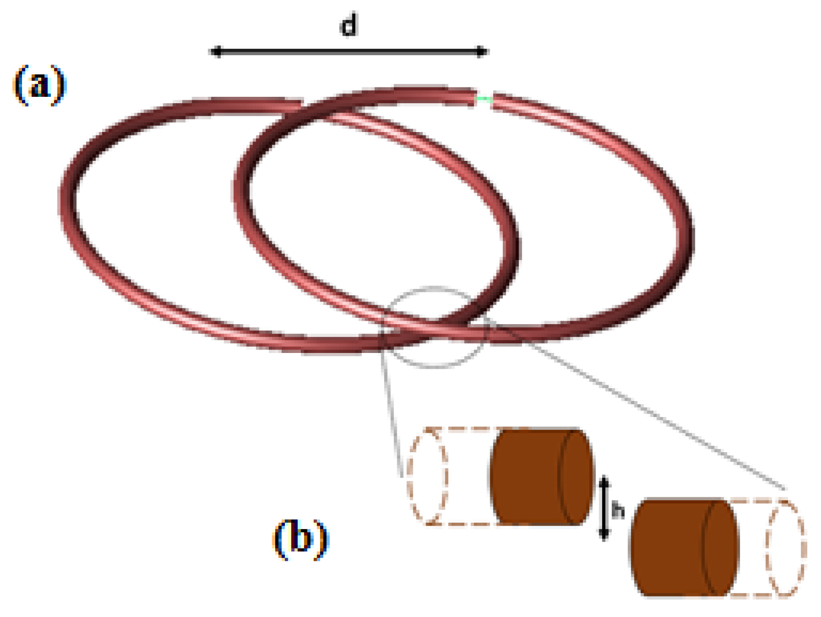
3.3. Phased-Array RF Coils

The mutual inductance between two conductors carrying currents J₁ and J₂ in the volumes V₁ and V₂ can be estimated, in the quasi-static approximation, with the following expression [2]:

$$M=\frac{{\mu }_0}{4\pi I_1{I}_2}{{\displaystyle \iiint }}_{V_1}{{\displaystyle \iiint }}_{V_2}\frac{J_1\left(r\right)\cdot J_2\left(r^{\prime }\right)}{R}dvd{v}^{\prime }$$

(19)

where I₁ and I₂ represent the total current in V₁ and V₂, respectively, and $R=\left|r-r^{\prime }\right|$.

This equation has been largely employed for the calculation of the mutual inductance between two circular [37] or square [16,38] loops constituting a dual-element phased-array coil by taking into account the conductor’s geometry. Moreover, from Equation (19) can be derived a simplified formulation for the calculation of the mutual inductance between two parallel conductors with the same length l and placed at distance d [2]:

$$M_{cond}=\frac{{\mu }_{0}l}{2\pi }\left[ln\left(\frac{l}{d}+\sqrt{1+\frac{l^2}{d^2}}\right)-\sqrt{1+\frac{d^2}{l^2}}+\frac{d}{l}\right]$$

(20)

In this work, analytical and numerical simulations were performed for a two-element phased array (Coil #6) made by two 52.5 mm-radius circular loops with 2 mm-radius wire. The analytical calculation of the mutual inductance between the two circular loops was performed using Equation (19), which becomes equal to Equation (10) with the addition of the distances between the loop centers (d) and between the loop planes (h).

In the FDTD simulation (Figure 6a), a tuning capacitor and a 50 Ω port were inserted in the first loop, inserting the same tuning capacitor and a passive load (50 Ω) in the second loop. Decoupling between the two loops was assessed through the optimization of the S₂₁ scattering parameter as a function of the distance between the two coils. A receive-only two-element phased-array tuned at 21.3 MHz (0.5 T) designed for an open scanner (MROpen, Paramed srl, Genova, Italy) was simulated and tested [39].

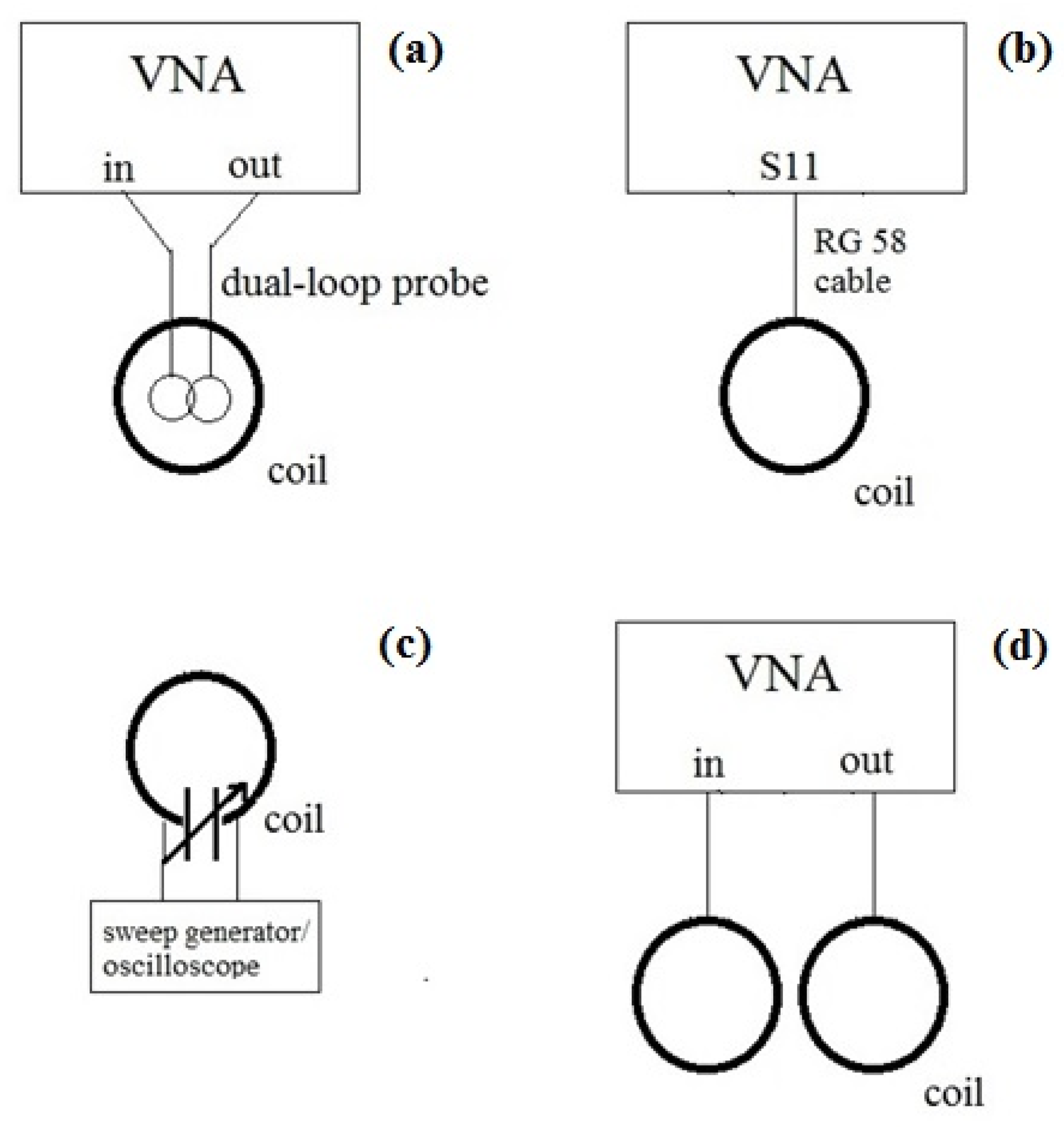
3.4. Workbench Tests

Workbench measurement on Coil #1 was performed with a network analyser HP3577 (Hewlett Packard, Palo Alto, CA, USA) acquiring the S₁₂ signal from a homemade dual-loop probe constituting two pick-up circular loops (diameter 20 mm) partially overlapped to minimize the in-air mutual inductive coupling (a condition achieved by separating the loop centres by 0.75 times their diameter [3]), see Figure 7a. The inductances of Coils #3–5 were measured by the S₁₁ parameter connecting the RF coil port to the network analyser via an RG58 coaxial cable, after performing a proper calibration (Figure 7b). Coil #2 was tested with an inductance measurement circuit (Figure 7c), placing the RF coil in parallel with a variable capacitor for creating a simple resonant tank circuit and successively performing resonant frequency measurement [10]. Finally, measurements on Coil #6 were performed by using one element of the array as a transmitter and the second one as a receiver, with both channels passively matched to 50 Ω, for estimation of the decoupling degree (Figure 7d).

4. Results and Discussion

Inductance simulations performed with the analytical and numerical (FDTD) methods were compared with experimental data obtained on the workbench to assess the accuracy.

Table 1. Measured and simulated inductance for different RF coils.

RF Coil Design (Nuclei, Main Field)	Experimental Inductance (nH) ± 2%	Analytical Inductance (nH)	FDTD Inductance (nH) ± 0.1%
Coil #1 Lowpass Birdcage (1H, 0.18 T)	114	121	115
Coil #2 Solenoid (1H, 7 T)	161	163	164
Coil #3 Circular coil (1H, 3 T)	235	224	231
Coil #4 Circular coil (13C, 3 T)	146	142	147
Coil #5 Elliptical coil (1H, 3 T)	78	74	76

summarizes the inductance values obtained with the workbench, analytical and FDTD methods, comprising the maximum inductance errors associated with each reported value. The errors associated with the analytical method are assumed to be negligible, since the inductance calculations are performed by implementing analytical equations with well-defined parameters. The errors associated with the FDTD method depend on the mesh density and/or boundary conditions setup, and based on our experience they can generally be made less than 0.1%. The experimental errors are due to the measurement of the resonant frequencies and scattering coefficients (S₁₁, S₁₂) of the specific RF coil under consideration, and we estimate it to be about 2% for all the described RF coil designs.

The global inductance estimation of the lowpass birdcage RF Coil #1 was derived by measuring the tuning frequency on the workbench (8.1 MHz) and taking into account the calculated equivalent capacitance values [40]. The analytical and FDTD simulations provided a theoretical resonant frequency of about 7.8 MHz and 8.0 MHz, respectively. The comparison of experiment and theory provided inductance values (Table 1) with an error of about 4% (analytical) and 1% (FDTD). Coil #2 simulations were performed to verify the accuracy of the two estimation methods when the approximated formulae employed for inductance calculation failure [11]. As shown in Table 1, analytical (163 nH) and FDTD (164 nH) methods estimated inductance value of the solenoid RF coil #2 with an error of 1% and 2%, respectively, compared to the measured inductance (161 nH). Analytical simulations of the circular RF coils provided inductance results, with respect to the workbench data, presenting an error of about −5% (Coil #3) and −3% (Coil #4). The same comparison for the FDTD method showed an inductance value with an error of −2% (Coil #3) and 1% (Coil #4).

The analytical calculation of Coil #5 provided an inductance value with a difference with respect to the measured value of about −5%. FDTD simulation was performed by using an equivalent-width strip (w = 0.45 cm), and the inductance value was estimated with an error of about −3%.

The two loops’ (Coil #6) mutual-inductance determination via the analytical method, performed by using Equation (10) as function of the centers distance (d), provided a minimum value (optimal decoupling) for d = 82 mm [41], while the FDTD S₂₁ simulation showed optimum decoupling for a mutual distance between the two loops of 81 mm. Both results are within few % of the expected optimum decoupling distance equal to 0.75 times the coil diameter [4]. Workbench measurements confirmed decoupling maximization for an 81 mm center distance [41], in excellent agreement with the analytical and FDTD values (error less than 1%).

The two FDTD approach strategies reported in our work, when employed for simulating all the RF coil here considered, provided identical results. However, Method A (lossless tuning capacitor, ideal current feed port and Gaussian broadband pulse excitation) can be successfully employed for SNR estimation of RF coil loaded with lossy samples, since the use of a Gaussian pulse includes sample-induced resistance contribution. Conversely, Method B (non-resonant coil, 50 Ω port feed with sinusoidal current) is useful for calculating the magnetic field distribution [41].

5. Conclusions

This work presents a practical guide to estimating inductance for fast design of RF coils for magnetic resonance applications. To this purpose, we have presented a collection of useful analytical formulas for inductance estimation of the most used typologies of homemade RF coils, useful for targeted applications (volume, surface, phased array). They have the advantage of being easily implemented in a software code, providing the results in a very short time (seconds). It is worth noting that the inductance calculation with Equation (1) can be easily performed only for simple geometries, mainly for RF coils constituting linear or circular conductor segments.

The first validation of the above analytical approach employed an electromagnetic solver based on the FDTD algorithm that allows for the simulation of complex RF coil structures, without any geometry limitations. Moreover, the FDTD method allows us to incorporate in the computational domain the whole human body (or selected portions), providing simulations of more realistic MR experiments, although at the expense of longer computational time (hours).

Analytical and numerical inductance results were compared with workbench measurements performed on the most common volume and surface RF coil prototypes, tuned at a magnetic field ranging from 0.18 to 7 T. The comparison showed that both theoretical approaches provide inductance estimation with errors less than a few % with respect to the measured values. This demonstrates the feasibility of accurate inductance calculations that allows for a straightforward selection of the high-quality, non-magnetic tuning capacitors required for a fast-prototyping approach.

References

- Webb, A.G. Magnetic Resonance Technology: Hardware and System Component Design; The Royal Society of Chemistry: London, UK, 2016. [Google Scholar]
- Jin, J. Electromagnetic Analysis and Design in Magnetic Resonance Imaging; CRC: Boca Raton, FL, USA, 1999. [Google Scholar]
- Mispelter, J.; Lupu, M.; Briguet, A. NMR Probeheads for Biophysical and Biomedical Experiments: Theoretical Principles & Practical Guidelines, 2nd ed.; Imperial College Press: London, UK, 2015. [Google Scholar]
- Roemer, P.B.; Edelstein, W.A.; Hayes, C.E.; Souza, S.P.; Mueller, O.M. The NMR phased array. Magn. Reson. Med. 1990, 16, 192–225. [Google Scholar] [CrossRef] [PubMed]
- Ohliger, M.A.; Sodickson, D.K. An introduction to coil array design for parallel MRI. NMR Biomed 2006, 19, 300–315. [Google Scholar] [CrossRef] [PubMed]
- Wheeler, H.A. Simple inductance formulas for radio coils. Proc. Inst. Radio Eng. 1928, 16, 1398–1400. [Google Scholar] [CrossRef]
- Terman, F. Radio Engineering; McGraw-Hill: New York, NY, USA, 1937. [Google Scholar]
- Grover, F.W. Inductance Calculations; Dover: New York, NY, USA, 1962. [Google Scholar]
- Schormans, M.; Valente, M.; Demosthenous, A. Practical Inductive Link Design for Biomedical Wireless Power Transfer: A Tutorial. IEEE Trans. Biomed. Circuits Syst. 2018, 12, 1112–1130. [Google Scholar] [CrossRef] [PubMed] [Green Version]
- Rainey, J.K.; DeVries, J.S.; Sykes, B.D. Estimation and measurement of flat or solenoidal coil inductance for radiofrequency NMR coil design. J. Magn. Reson. 2007, 187, 27–37. [Google Scholar] [CrossRef] [PubMed]
- Thompson, M.T. Inductance calculation techniques-part I: Classical methods. Pow Control. Intel Mot. 1999, 25, 40–45. [Google Scholar]
- Doty, F.D. Probe design and construction. In Encyclopedia of NMR; John Wiley: New York, NY, USA, 1996; pp. 3753–3762. [Google Scholar]
- Giovannetti, G.; Landini, L.; Santarelli, M.F.; Positano, V. A fast and accurate simulator for the design of birdcage coils in MRI. Magn. Reson. Mater Phys Med. Biol. 2002, 15, 36–44. [Google Scholar] [CrossRef] [Green Version]
- Giovannetti, G.; Frijia, F. Inductance calculation in Magnetic Resonance solenoid coils with strip and wire conductors. Appl. Magn. Reson. 2020, 51, 703–710. [Google Scholar] [CrossRef]
- Giovannetti, G. Comparison between circular and square loops for low frequency Magnetic Resonance applications: Theoretical performance estimation. Concepts Magn. Reson. Part B 2016, 46B, 146–155. [Google Scholar] [CrossRef]
- Giovannetti, G.; Viti, V.; Positano, V.; Santarelli, M.F.; Landini, L.; Benassi, A. Magnetostatic simulation for accurate design of low field MRI phased-array coils. Concepts Magn. Reson. Part B 2007, 31B, 140–146. [Google Scholar] [CrossRef]
- Yee, K.S. Numerical solution of initial boundary value problems involving Maxwell’s equations in isotropic media. IEEE Trans. Antennas Propag. 1966, AP-14, 302. [Google Scholar]
- Amjad, A.; Kamondetdacha, R.; Kildishev, A.V.; Park, S.M. Power deposition inside a phantom for testing of MRI heating. IEEE Magn. 2005, 41, 4185–4187. [Google Scholar] [CrossRef]
- Wang, Z.; Lin, J.C.; Mao, W.; Liu, W.; Smith, M.B.; Collins, C.M. SAR and temperature: Simulations and comparison to regulatory limits for MRI. J. Magn. Reson. 2007, 26, 437–441. [Google Scholar] [CrossRef] [PubMed] [Green Version]
- Chen, J.; Feng, Z.; Jin, J.M. Numerical simulation of SAR and B/sub 1/-field inhomogeneity of shielded RF coils loaded with the human head. IEEE Trans. Biomed. Eng. 1998, 45, 650–659. [Google Scholar] [CrossRef]
- Hartwig, V.; Giovannetti, G.; Vanello, N.; Landini, L.; Santarelli, M.F. Numerical Calculation of Peak-to-Average Specific Absorption Rate on Different Human Thorax Models for Magnetic Resonance Safety Considerations. Appl. Magn. Reson. 2010, 38, 337–348. [Google Scholar] [CrossRef]
- Giovannetti, G.; Hartwig, V.; Frijia, F.; Menichetti, L.; Positano, V.; Ardenkjaer-Larsen, J.H.; Lionetti, V.; Aquaro, G.D.; De Marchi, D.; Flori, A.; et al. Hyperpolarized 13C MRS Cardiac Metabolism Studies in Pigs: Comparison Between Surface and Volume Radiofrequency Coils. Appl. Magn. Reson. 2012, 42, 413–428. [Google Scholar] [CrossRef]
- Giovannetti, G.; Wang, Y.; Tumkur Jayakumar, N.K.; Barney, J.; Tiberi, G. Magnetic Resonance Wire Coil Losses Estimation with Finite-Difference Time-Domain Method. Electronics 2022, 11, 1872. [Google Scholar] [CrossRef]
- Hayes, C.E.; Edelstein, W.A.; Schenck, J.F.; Mueller, O.M.; Eash, M. An efficient, highly homogeneous radiofrequency coil for whole-body NMR imaging at 1.5 T. J. Magn Reson. 1985, 63, 622–628. [Google Scholar] [CrossRef]
- Vullo, T.; Zipagan, R.T.; Pascone, R.; Whalen, J.P.; Cahill, P.T. Experimental design and fabrication of birdcage resonators for magnetic resonance imaging. Magn. Reson. Med. 1992, 24, 243–252. [Google Scholar] [CrossRef]
- Isaac, G.; Schnall, M.D.; Lenkinski, R.E.; Vogele, K. A design for a double-tuned birdcage coil for use in an integrated MRI/MRS examination. J. Magn. Reson. 1990, 89, 41–50. [Google Scholar] [CrossRef]
- Rath, A.R. Design and performance of a double-tuned birdcage coil. J. Magn. Reson. 1990, 86, 488–495. [Google Scholar]
- Murphy-Boesch, J.; Srinivasan, R.; Carvajal, L.; Brown, T.R. Two configurations of the four-ring birdcage coil for 1H imaging and 1H-decoupled 31P spectroscopy of the human head. J. Magn. Reson. B 1994, 103, 103–114. [Google Scholar] [CrossRef] [PubMed]
- Fantasia, M.; Galante, A.; Maggiorelli, F.; Retico, A.; Fontana, N.; Monorchio, A.; Alecci, M. Numerical and workbench design of 2.35 T double-tuned (1H/23Na) nested RF birdcage coils suitable for animal size MRI. IEEE Trans. Med. Imaging 2020, 39, 3175–3186. [Google Scholar] [CrossRef] [PubMed]
- Pascone, R.J.; Garcia, B.J.; Fitzgerald, T.M.; Vullo, T.; Zipagan, R.; Cahill, P.T. Generalized electrical analysis of low-pass and high-pass birdcage resonators. Magn. Reson. Imaging 1991, 9, 395–408. [Google Scholar] [CrossRef]
- Chen, C.N.; Hoult, D.I. Biomedical Magnetic Resonance Technology; Taylor & Francis: Oxford, UK, 1989. [Google Scholar]
- Giovannetti, G.; Frijia, F.; Flori, A.; Montanaro, D. Design and simulation of a Helmholtz Coil for Magnetic Resonance Imaging and Spectroscopy experiments with a 3T MR clinical scanner. Appl. Magn. Reson. 2019, 50, 1083–1097. [Google Scholar] [CrossRef]
- Frijia, F.; Flori, A.; Giovannetti, G. Design, simulation, and test of surface and volume radio frequency coils for 13C magnetic resonance imaging and spectroscopy. Rev. Sci. Instrum. 2021, 92, 081402. [Google Scholar] [CrossRef]
- Cooke, N. Self-inductance of the elliptical loop. Proc. IEEE 1963, 110, 1293–1298. [Google Scholar] [CrossRef]
- Wolfram MathWorld. Available online: http://mathworld.wolfram.com/HypergeometricFunction.html (accessed on 22 December 2021).
- Giovannetti, G.; Flori, A.; De Marchi, D.; Matarazzo, G.; Frijia, F.; Burchielli, S.; Montanaro, D.; Aquaro, G.D.; Menichetti, L. Simulation, design, and test of an elliptical surface coil for magnetic resonance imaging and spectroscopy. Concepts Magn. Reson. Part B 2017, 47B, e21361. [Google Scholar] [CrossRef] [Green Version]
- Giovannetti, G. A theoretical study on circular wire and flat strip conductor inductance for Magnetic Resonance shielded phased-array circular coils. Appl. Magn Reson. 2019, 50, 1391–1398. [Google Scholar] [CrossRef]
- Giovannetti, G. Mutual inductance in Magnetic Resonance two-element phased-array square coils with strip and wire conductors. Appl. Magn. Reson. 2021, 52, 135–142. [Google Scholar] [CrossRef]
- Hartwig, V.; Vivoli, G.; Tassano, S.; Carrozzi, A.; Giovannetti, G. Decoupling and shielding numerical optimization of MRI phased-array coils. Measurement 2016, 82, 450–460. [Google Scholar] [CrossRef]
- Giovannetti, G. Birdcage Coils: Equivalent capacitance and equivalent inductance. Concepts Magn. Reson. Part B 2014, 44B, 32–38. [Google Scholar] [CrossRef]
- Hartwig, V.; Tassano, S.; Mattii, A.; Vanello, N.; Positano, V.; Santarelli, M.F.; Landini, L.; Giovannetti, G. Computational analysis of a radiofrequency knee coil for low-field MRI using FDTD. Appl. Magn. Reson. 2013, 44, 389–400. [Google Scholar] [CrossRef]