Cooperative Localization Based on Augmented State Belief Propagation for Mobile Agent Networks

Abstract

Belief propagation (BP) is widely used to solve the cooperative localization problem due to its excellent performance and natural distributed structure of implementation. For a mobile agent network, its factor graph inevitably encounters loops. In this case, the BP algorithm becomes iterative and can only provide an approximate marginal probability density function of the estimate with finite iterations. We propose an augmented-state BP algorithm for mobile agent networks to alleviate the effect of loops. By performing state augmentation, the messages in the factor graph will actually be allowed to be backward propagated, which reduces the number of loops in the factor graph, increases the available information of agents, and thus, benefits the localization. Experimental results demonstrate the better performance of the proposed algorithm over the original BP method.

1. Introduction

Location awareness promotes the rapid development of autonomous driving [1], formation flying [2], robotics [3], etc. Accurate location estimation is a prerequisite for proper functioning control loops [4,5]. Traditionally, agents can perform localization tasks through the global positioning system (GPS) or beacon localization. However, localization by GPS requires continuous and stable GPS signal reception, which is usually impossible in harsh scenarios, e.g., when indoors or when the signal is jammed. On the other hand, beacon localization requires a large number of anchors with known location and is impractical due to its high cost. Another way to perform localization is to use inertial measurement units (IMUs) and dead reckoning (DR), but the unlimited increase of accumulated errors is often unacceptable [6]. In recent years, cooperative localization (CL) has received extensive attention due to its broad applicability. CL uses relative measurements among neighboring agents to improve the absolute position of each agent in the network. Compared with noncooperative localization (NCL), CL can achieve better-precision localization of the entire agent network with some additional computation and communication [7,8]. The advantages of CL are more obvious, especially for heterogeneous agent networks. For example, a small number of agents equipped with high-precision sensors can share information with other agents to benefit the entire agent network through the master-slave CL algorithm [9].

Various CL algorithms have been investigated in the existing work [10,11,12,13,14,15], among which, a message-passing algorithm called belief propagation (BP) [14,15] is the most popular for its high-precision localization and natural distributed architecture of implementation. The original BP algorithm involves complex integration, product operations, and transmission of probability density functions (pdfs), so it cannot be directly applied in practice. For the case of linear models and Gaussian noise, the Gaussian BP [16,17] is a reduced and simplified version that can be easily implemented. However, it cannot handle real-world scenarios of nonlinear measurements and non-Gaussian noise. For that case, one effective approach is nonparametric belief propagation (NBP) [18,19]. As a generalization of particle filters, NBP uses particle representation [20] to approximate the incoming and outgoing messages of agents and thus can handle noise with arbitrary distribution and nonlinear measurements. However, a small number of particles are inadequate to provide satisfactory estimation accuracy, and too many particles will cause unacceptable communicational and computational burden. Ref. [21] proposed to propagate the beliefs instead of the messages, and used Gaussian mixture density with fewer components to approximate the beliefs. In this way, each agent can perform broadcast instead of peer-to-peer communication, which greatly reduces the communication overhead, requiring only a little extra computation. In Ref. [22], NBP was investigated in an anchor-free environment, and an intermittent BP framework based on dead reckoning was proposed, which naturally combined CL and NCL algorithms. Since the accumulated error of IMU was considered in the prediction process, the localization accuracy was further improved. In Refs. [23,24], the posterior linearization filter and the unscented Kalman filter were integrated with BP to deal with nonlinear measurements. Compared with NBP, these two methods also have satisfactory performance but less computation and communication. In Refs. [25,26], Two BP algorithms based on non-Gaussian ranging models were proposed to deal with non-Gaussian noise.

BP has demonstrated its powerful capabilities in CL. However, as a message-passing algorithm based on factor graphs, BP can only provide the optimal results when there is no loop in the factor graph. Otherwise, BP becomes iterative and can only obtain approximate solutions [27]. Further, for mobile agent networks, the existing methods based on BP merely allow forward message passing and thus neglect the loops across time. This definitely sacrifices the accuracy of localization. In this paper, we propose an augmented state BP algorithm for mobile agent networks, which realizes a backward propagation of messages by performing state augmentation. This backward propagation (or retrodiction) in essence reduces the number of loops in the factor graph, increases the available information at each agent, and thus improves the accuracy of localization. Considering the computational and communicational burden, we suggest to use a few limited steps of retrodiction. Besides the proposed augmented BP, the contribution of this paper includes the formulation of the CL problem under the assumption that each agent has a dynamic motion model. Different from formulations of the existing CL work, this assumption actually considers the prior motion information of agents. Our formulation can reduce to the existing ones by setting an extremely large covariance of process noise in the dynamic model. Thus, our formulation is more general. We also provide the corresponding centralized fusion algorithm for the formulated CL problem, which acts as a benchmark for evaluating the distributed CL algorithms. Experimental results demonstrate the effectiveness and advantage of our algorithm.

The paper is organized as follows. Section 2 describes the system model and formulates the CL problem. Section 3 provides the centralized fusion algorithm for the formulated CL problem. Section 4 briefly reviews the BP algorithm. Section 5 proposes the augmented state BP algorithm. Experimental results are given in Section 6. Section 7 concludes the paper.

2. System Model and Problem Formulation

Consider $N$ agents in a two-dimensional plane in a GPS-denied scenario without any anchors. The set of agents is denoted as $\mathcal{A}$. Each agent moves according to the following dynamic model

$${\mathit{x}}_{k+1}^i={\mathit{F}}_k^i{\mathit{x}}_k^i+{\mathit{G}}_k^i{\mathit{w}}_k^i,i\in \mathcal{A}$$

(1)

where ${\mathit{x}}_k^i={[x_k^i,{\dot{x}}_k^i,y_k^i,{\dot{y}}_k^i]}^{\mathrm{T}}$ is the state of the $i\mathrm{th}$ agent at time $k$, and $x_k^i$, ${\dot{x}}_k^i$ and $y_k^i$, ${\dot{y}}_k^i$ are the horizontal and vertical positions and velocities, respectively. The process noise ${\mathit{w}}_k^i$ is assumed white and Gaussian-distributed with zero mean and covariance ${\mathit{Q}}_k^i$. The process noises are assumed independent across agents. The initial state ${\mathit{x}}_0^i$ is also assumed Gaussian-distributed and independent across agents. It is assumed that each agent $i\in \mathcal{A}$ can measure its own position and/or velocity increments with respect to a geostationary coordinate frame. The internal measurement of the $i\mathrm{th}$ agent at time $k$ is modeled as

$${\mathit{z}}_k^i={\mathit{H}}_k^i({\mathit{x}}_k^i-{\mathit{x}}_{k-1}^i)+{\mathit{v}}_k^i,i\in \mathcal{A}$$

(2)

where ${\mathit{H}}_k^i$ and ${\mathit{v}}_k^i$ indicate the measurement matrix of the $i\mathrm{th}$ agent at time $k$ and the corresponding measurement noise, respectively. When ${\mathit{H}}_k^i=\left[\begin{array}{cccc}1& 0& 0& 0\\ 0& 0& 1& 0\end{array}\right]$, ${\mathit{z}}_k^i$ is called displacement measurement, which is a special case of model (2). The measurement noise ${\mathit{v}}_k^i$ is assumed to be white Gaussian with zero mean and covariance ${\mathit{R}}_k^i$. Certain pairs of agents, say $i,j\in \mathcal{A}$, can obtain inter-agent measurements ${\mathit{z}}_k^{i.j}$, called relative measurements. Two agents having relative measurements are called neighbors and it is assumed that information can only be shared among neighbors. Denote by ${\mathcal{N}}_{i,k}$ the set of neighbors of agent $i$ at time $k$. The relative measurements have the following model

$${\mathit{z}}_k^{i.j}={\mathit{H}}_k^{i.j}({\mathit{x}}_k^j-{\mathit{x}}_k^i)+{\mathit{v}}_k^{i.j},i\in \mathcal{A},j\in {\mathcal{N}}_{i,k}$$

(3)

where ${\mathit{v}}_k^{i.j}$ is the corresponding measurement noise and is assumed to be white Gaussian with zero mean and covariance ${\mathit{R}}_k^{i,j}$. All measurement noises, process noises and initial states are assumed mutually independent.

Let

$${\mathit{Z}}_k\triangleq {[{({\mathit{Z}}_k^{\mathrm{self}})}^{\mathrm{T}},{({\mathit{Z}}_k^{\mathrm{rel}})}^{\mathrm{T}}]}^{\mathrm{T}}$$

(4)

where

$$\begin{array}{l}{\mathit{Z}}_k^{\mathrm{self}}\triangleq {[{({\mathit{z}}_k^1)}^{\mathrm{T}},\dots ,{({\mathit{z}}_k^N)}^{\mathrm{T}}]}^{\mathrm{T}}\\ {\mathit{Z}}_k^{\mathrm{rel}}\triangleq {[{({\mathit{Z}}_k^{1,\mathrm{rel}})}^{\mathrm{T}},\dots ,{({\mathit{Z}}_k^{N,\mathrm{rel}})}^{\mathrm{T}}]}^{\mathrm{T}}\\ {\mathit{Z}}_k^{i,\mathrm{rel}}\triangleq {[{\mathit{z}}_k^{i,j_1},\cdots ,{\mathit{z}}_k^{i,j_{n_i}}]}^{\mathrm{T}},j_1,\cdots ,j_{n_i}\in {\mathcal{N}}_{i,k}\end{array}$$

and $n_i$ is the number of neighbors of agent $i$. The problem considered is to use all available measurements including the internal measurements and the inter-agent relative measurements to estimate the states of all agents, i.e.,

$${\hat{\mathit{X}}}_k=E[{\mathit{X}}_k|{\mathit{Z}}_k]$$

where ${\mathit{X}}_k\triangleq {[{({\mathit{x}}_k^1)}^{\mathrm{T}},\dots ,{({\mathit{x}}_k^N)}^{\mathrm{T}}]}^{\mathrm{T}}$ and $E[\cdot ]$ denotes the minimum mean-squared error (MMSE) estimator. Note that the stacking way of the measurements in Equation (4) is for the convenience of developing of filtering algorithm. The linear Gaussian assumptions made through Equations (1)–(3) do not reduce the significance of our study, since our proposed algorithm can be directly combined with NBP to deal with nonlinear or non-Gaussian cases.

Remark 1.

The major difference between our formulation and the existing ones (see, e.g., Ref. [28]) lies in the assumption of dynamic models of agents, i.e., Equation (1). Traditionally, the displacement measurement model is commonly used as the dynamic model by viewing the displacement measurement ${\mathit{z}}_k^i$as known inputs, i.e.,

$$\left[\begin{array}{c}{x}_k^i\\ y_k^i\end{array}\right]=\left[\begin{array}{c}{x}_{k-1}^i\\ y_{k-1}^i\end{array}\right]+{\mathit{z}}_k^i-{\mathit{v}}_k^i$$

Thus, the information from displacement measurements is actually utilized in the prediction step of the filter. In our formulation, the internal measurement Equation (2), including displacement model as a special case, is more general. Another advantage of our formulation is that the prior motion information of agents can be adopted in the filtering algorithm to improve the localization performance. If such information is unavailable, we can simply set a large enough ${\mathit{Q}}_k^i$to represent that we have very little faith in the dynamic model and it naturally has slight effect on the estimation results. Thus, intuitively, our formulation reduces to the existing ones by setting a large enough ${\mathit{Q}}_k^i$.

3. Centralized Fusion

The centralized fusion, which utilizes all measurements from all agents to estimate the states of all agents at the fusion center, can provide the optimal state estimates [29]. The optimal centralized fusion in the best linear unbiased estimation (BLUE) sense for the formulation without the assumption of agents’ dynamic models is given in Ref. [28]. Therein, the system states are viewed as non-random unknown quantities, which is different from ours. Next, we investigate the centralized fusion for our formulated problem.

Stacking states and measurements from all agents, we have the following dynamic model

$${\mathit{X}}_{k+1}={\mathit{F}}_k{\mathit{X}}_k+{\mathit{G}}_k{\mathit{w}}_k$$

(5)

$${\mathit{Z}}_k={\mathit{H}}_k^{\mathrm{c}}{\mathit{X}}_k-{\mathit{H}}_k^p{\mathit{X}}_{k-1}+{\mathit{V}}_k$$

(6)

where

$$\begin{array}{l}{\mathit{F}}_k=\mathrm{diag}({\mathit{F}}_k^1,\dots ,{\mathit{F}}_k^N),{\mathit{G}}_k=\mathrm{diag}({\mathit{G}}_k^1,\dots ,{\mathit{G}}_k^N)\\ {\mathit{w}}_k={[{({\mathit{w}}_k^1)}^{\mathrm{T}},\dots ,{({\mathit{w}}_k^N)}^{\mathrm{T}}]}^{\mathrm{T}},{\mathit{H}}_k^{\mathrm{c}}={[{({\mathit{H}}_k^{\mathrm{self}})}^{\mathrm{T}},{({\mathit{H}}_k^{\mathrm{rel}})}^{\mathrm{T}}]}^{\mathrm{T}}\\ {\mathit{H}}_k^p={[{({\mathit{H}}_k^{\mathrm{self}})}^{\mathrm{T}},\mathbf{0}]}^{\mathrm{T}},{\mathit{V}}_k={[{({\mathit{v}}_k^1)}^{\mathrm{T}},\dots ,{({\mathit{v}}_k^N)}^{\mathrm{T}},{({\mathit{v}}_k^{1,\mathrm{rel}})}^{\mathrm{T}},\dots ,{({\mathit{v}}_k^{N,\mathrm{rel}})}^{\mathrm{T}}]}^{\mathrm{T}}\\ {\mathit{v}}_k^{i,\mathrm{rel}}={[{\mathit{v}}_k^{i,j_1},\cdots ,{\mathit{v}}_k^{i,j_{n_i}}]}^{\mathrm{T}},j_1,\cdots ,j_{n_i}\in {\mathcal{N}}_{i,k}\end{array}$$

The matrix ${\mathit{H}}_k^{\mathrm{self}}$ corresponding to the internal measurements is given by

$${\mathit{H}}_k^{\mathrm{self}}=\mathrm{diag}({\mathit{H}}_k^1,\dots ,{\mathit{H}}_k^N)$$

The matrix ${\mathit{H}}_k^{\mathrm{rel}}$ corresponding to the relative measurements is determined by the concrete topology of the network. Taking the chain topology as an example, we have

$${\mathit{H}}_k^{\mathrm{rel}}=\left[\begin{array}{ccccc}-{\mathit{H}}_k^{1,2}& {\mathit{H}}_k^{1,2}& & & \\ {\mathit{H}}_k^{2,1}& -{\mathit{H}}_k^{2,1}& & & \\ & -{\mathit{H}}_k^{2,3}& {\mathit{H}}_k^{2,3}& & \\ & & & \ddots & \\ & & & {\mathit{H}}_k^{N,N-1}& -{\mathit{H}}_k^{N,N-1}\end{array}\right]$$

The state estimation of system Equations (5) and (6) consists of two steps: prediction and update. The state prediction is calculated as

$${\hat{\mathit{X}}}_{k+1|k}={\mathit{F}}_k{\hat{\mathit{X}}}_{k|k}$$

(7)

$${\mathit{P}}_{k+1|k}={\mathit{F}}_k{\mathit{P}}_{k|k}{\mathit{F}}_k^{\mathrm{T}}+{\mathit{G}}_k{\mathit{Q}}_k{\mathit{G}}_k^{\mathrm{T}}$$

(8)

where ${\mathit{Q}}_k=\mathrm{diag}({\mathit{Q}}_k^1,\dots ,{\mathit{Q}}_k^N)$ is the covariance matrix of ${\mathit{w}}_k$.

For the update step, the normal update in the Kalman filter cannot be used since the measurement ${\mathit{Z}}_{k+1}$ is also related to ${\mathit{X}}_k$ as shown in Equation (6). Next, we use the linear MMSE (LMMSE) estimator [30], which is also optimal in the MMSE sense due to the linear Gaussian assumptions made in this paper, and the update can be calculated as

$${\hat{\mathit{X}}}_{k+1|k}={\mathit{F}}_k{\hat{\mathit{X}}}_{k|k}{\hat{\mathit{X}}}_{k+1|k+1}=E[{\mathit{X}}_{k+1}|{\mathit{Z}}_{k+1}]={\hat{\mathit{X}}}_{k+1|k}+{\mathit{C}}_{k+1}{\mathit{S}}_{k+1}^{-1}({\mathit{Z}}_{k+1}-{\hat{\mathit{Z}}}_{k+1|k})$$

(9)

and

$${\mathit{P}}_{k+1|k+1}=\mathrm{MSE}({\hat{\mathit{X}}}_{k+1|k+1})={\mathit{P}}_{k+1|k}-{\mathit{C}}_{k+1}{\mathit{S}}_{k+1}^{-1}{\mathit{C}}_{k+1}^T$$

(10)

where MSE denotes the mean-square error matrix. From Equation (6), the measurement prediction is

$${\hat{\mathit{Z}}}_{k+1}={\mathit{H}}_{k+1}^{\mathrm{c}}{\hat{\mathit{X}}}_{k+1|k}-{\mathit{H}}_{k+1}^p{\hat{\mathit{X}}}_{k|k}$$

(11)

and

$$\begin{array}{ll}{\mathit{S}}_{k+1}& =E[({\mathit{Z}}_{k+1}-{\hat{\mathit{Z}}}_{k+1|k}){({\mathit{Z}}_{k+1}-{\hat{\mathit{Z}}}_{k+1|k})}^{\mathrm{T}}]\\ & =E[({\mathit{H}}_{k+1}^{\mathrm{c}}{\hat{\mathit{X}}}_{k+1|k}-{\mathit{H}}_{k+1}^p{\hat{\mathit{X}}}_{k|k}+{\mathit{v}}_k){({\mathit{H}}_{k+1}^{\mathrm{c}}{\hat{\mathit{X}}}_{k+1|k}-{\mathit{H}}_{k+1}^p{\hat{\mathit{X}}}_{k|k}+{\mathit{v}}_k)}^{\mathrm{T}}]\\ & ={\mathit{R}}_k+{\mathit{H}}_{k+1}^{\mathrm{c}}{\mathit{P}}_{k+1|k}{({\mathit{H}}_{k+1}^{\mathrm{c}})}^{\mathrm{T}}+{\mathit{H}}_{k+1}^p{\mathit{P}}_{k|k}{({\mathit{H}}_{k+1}^p)}^{\mathrm{T}}\\ & -{\mathit{H}}_{k+1}^{\mathrm{c}}{\mathit{F}}_k{\mathit{P}}_{k|k}{({\mathit{H}}_{k+1}^p)}^{\mathrm{T}}-{\mathit{H}}_{k+1}^p{\mathit{P}}_{k|k}{\mathit{F}}_k^{\mathrm{T}}{({\mathit{H}}_{k+1}^{\mathrm{c}})}^{\mathrm{T}}\end{array}$$

(12)

where ${\mathit{R}}_k=E[{\mathit{V}}_k{\mathit{V}}_k^{\mathrm{T}}]$. The cross-covariance ${\mathit{C}}_{k+1}$ is

$$\begin{array}{ll}{\mathit{C}}_{k+1}& =E[({\mathit{X}}_{k+1}-{\hat{\mathit{X}}}_{k+1|k}){({\mathit{Z}}_{k+1}-{\hat{\mathit{Z}}}_{k+1|k})}^{\mathrm{T}}]\\ & =E[{\hat{\mathit{X}}}_{k+1|k}{({\mathit{H}}_{k+1}^{\mathrm{c}}{\hat{\mathit{X}}}_{k+1|k}-{\mathit{H}}_{k+1}^p{\hat{\mathit{X}}}_{k|k}+{\mathit{v}}_{k+1})}^{\mathrm{T}}]\\ & ={\mathit{P}}_{k+1|k}{({\mathit{H}}_{k+1}^{\mathrm{c}})}^{\mathrm{T}}-{\mathit{F}}_k{\mathit{P}}_{k|k}{({\mathit{H}}_{k+1}^p)}^{\mathrm{T}}\end{array}$$

(13)

Substituting Equations (11)–(13) into Equations (9) and (10), we can get

$${\hat{\mathit{X}}}_{k+1|k+1}={\hat{\mathit{X}}}_{k+1|k}+{\mathit{W}}_{k+1}({\mathit{Z}}_{k+1}-{\hat{\mathit{Z}}}_{k+1|k})$$

(14)

$${\mathit{P}}_{k+1|k+1}={\mathit{P}}_{k+1|k}-{\mathit{W}}_{k+1}{\mathit{S}}_{k+1}{\mathit{W}}_{k+1}^{\mathrm{T}}$$

(15)

where the filter gain ${\mathit{W}}_{k+1}$ is given by

$${\mathit{W}}_{k+1}={\mathit{C}}_{k+1}{\mathit{S}}_{k+1}^{-1}=({\mathit{P}}_{k+1|k}{({\mathit{H}}_{k+1}^{\mathrm{c}})}^{\mathrm{T}}-{\mathit{F}}_k{\mathit{P}}_{k|k}{({\mathit{H}}_{k+1}^p)}^{\mathrm{T}}){\mathit{S}}_{k+1}^{-1}$$

The centralized fusion Equation (9) can achieve the best performance in the MMSE sense, but it needs to transmit all measurements to the fusion center, which is impossible in practice especially for mobile agent networks.

4. BP-Based Cooperative Localization

In this section, we briefly introduce the BP algorithm, which serves as the basis for our augmented state BP discussed in the next section. The procedures of BP are presented in a general form with pdfs. For the linear Gaussian case, these pdfs are all Gaussian, and BP can be implemented with the first two-order moments straightforwardly.

The MMSE estimates of each agent is

$${\hat{\mathit{x}}}_k^i=\int {\mathit{x}}_k^{i}f({\mathit{x}}_k^i|{\mathit{Z}}_{1:k})d{\mathit{x}}_k^i$$

(16)

where ${\mathit{Z}}_{1:k}$ is all measurements up to time $k$. Obtaining $f({\mathit{x}}_k^i|{\mathit{Z}}_{1:k})$ involves the marginalization of the joint pdf $f({\mathit{X}}_{0:k}|{\mathit{Z}}_{1:k})$, where ${\mathit{X}}_{0:k}\triangleq {[{({\mathit{X}}_0)}^{\mathrm{T}},\dots ,{({\mathit{X}}_k)}^{\mathrm{T}}]}^{\mathrm{T}}$. Since its computational complexity increases exponentially with the size of the agent network, direct marginalization is infeasible. To solve this problem, BP provides an effective way. According to the independent assumption, the joint pdf $f({\mathit{X}}_{0:k}|{\mathit{Z}}_{1:k})$ can be factorized into

$$f({\mathit{X}}_{0:k}|{\mathit{Z}}_{1:k})\propto {\displaystyle \prod }_{i\in \mathcal{A}}f({\mathit{x}}_0^i){\displaystyle \prod }_{t=1}^k{\displaystyle \prod }_{i_1\in \mathcal{A}}f({\mathit{x}}_t^{i_1}|{\mathit{x}}_{t-1}^{i_1})f({\mathit{z}}_t^{i_1}|{\mathit{x}}_t^{i_1},{\mathit{x}}_{t-1}^{i_1}){\displaystyle \prod }_{j\in {\mathcal{N}}_{i_1,k}}f({\mathit{z}}_t^{i_1,j}|{\mathit{x}}_t^{i_1},{\mathit{x}}_t^j)$$

(17)

Equation (17) is mapped to the factor graph as shown in Figure 1. A factor graph $\mathcal{G}=(\mathcal{V},ℰ)$ is composed of nodes $\mathcal{V}$ and edges $ℰ$. The nodes are divided into factor nodes and variable nodes. Factor nodes are represented by boxes, which are associated with $f({\mathit{z}}_k^i|{\mathit{x}}_k^i,{\mathit{x}}_{k-1}^i)f({\mathit{x}}_k^i|{\mathit{x}}_{k-1}^i)$ or $f({\mathit{z}}_k^{i,j},{\mathit{z}}_k^{j,i}|{\mathit{x}}_k^i,{\mathit{x}}_k^j)$, and variable nodes are represented by circles, which are associated with ${\mathit{x}}_k^i$. Each edge connects the factor node with its related variable nodes. The BP algorithm propagates messages along the edges on the factor graph to calculate the belief $b({\mathit{x}}_k^i)$ corresponding to each variable node ${\mathit{x}}_k^i$. For the case of loop-free factor graph, the beliefs are the exact conditional marginal pdfs, i.e., $b({\mathit{x}}_k^i)=f({\mathit{x}}_k^i|{\mathit{Z}}_{1:k})$. Otherwise, the BP becomes iterative and can only provide an approximated solution. It is not ensured that, by iterations, the BP will converge, although it usually converges in many cases [23,27]. In real practice, a number of iterations are commonly performed.

For the $p\mathrm{th}$ iteration, the belief is given by

$$b^p({\mathit{x}}_k^i)\propto m_{\to k}({\mathit{x}}_k^i){\displaystyle \prod }_{j\in {\mathcal{N}}_{i,k}}{m}_{j\to i}^p({\mathit{x}}_k^i),i\in \mathcal{A}$$

(18)

where $m_{\to k}({\mathit{x}}_k^i)$ is the messages propagated from variable node ${\mathit{x}}_{k-1}^i$ to variable node ${\mathit{x}}_k^i$

$$m_{\to k}({\mathit{x}}_k^i)\propto \int f({\mathit{z}}_k^i|{\mathit{x}}_k^i,{\mathit{x}}_{k-1}^i)f({\mathit{x}}_k^i|{\mathit{x}}_{k-1}^i)b^p({\mathit{x}}_{k-1}^i)d{\mathit{x}}_{k-1}^i$$

(19)

and $m_{j\to i}^p({\mathit{x}}_k^i)$ is the message propagated from the factor node $f({\mathit{z}}_k^{i,j},{\mathit{z}}_k^{j,i}|{\mathit{x}}_k^i,{\mathit{x}}_k^j)$ to variable node ${\mathit{x}}_k^i$

$$m_{j\to i}^p({\mathit{x}}_k^i)\propto {\displaystyle \int f({\mathit{z}}_k^{i,j},{\mathit{z}}_k^{j,i}|{\mathit{x}}_k^i,{\mathit{x}}_k^j)n_{j\to i}^{p-1}({\mathit{x}}_k^j)d{\mathit{x}}_k^j,j\in {\mathcal{N}}_{i,k}}$$

(20)

with

$$n_{j\to i}^{p-1}({\mathit{x}}_k^j)\propto m_{\to k}({\mathit{x}}_k^j){\displaystyle \prod }_{l\in {\mathcal{N}}_{j,k}\backslash i}{m}_{l\to j}^{p-1}({\mathit{x}}_k^j)$$

(21)

Note that since Equation (3) distinguishes between ${\mathit{z}}_k^{i,j}$ and ${\mathit{z}}_k^{j,i}$, the conditional joint pdf of ${\mathit{z}}_k^{i,j}$ and ${\mathit{z}}_k^{j,i}$ is used in Equation (20). The iteration starts with $n_{j\to i}^0({\mathit{x}}_k^j)=m_{\to k}({\mathit{x}}_k^j)$. When $b({\mathit{x}}_k^i)$, i.e., the posterior $f({\mathit{x}}_k^i|{\mathit{Z}}_{1:k})$, is obtained, we can get the approximate MMSE estimate of ${\mathit{x}}_k^i$.

5. Augmented State BP Cooperative Localization

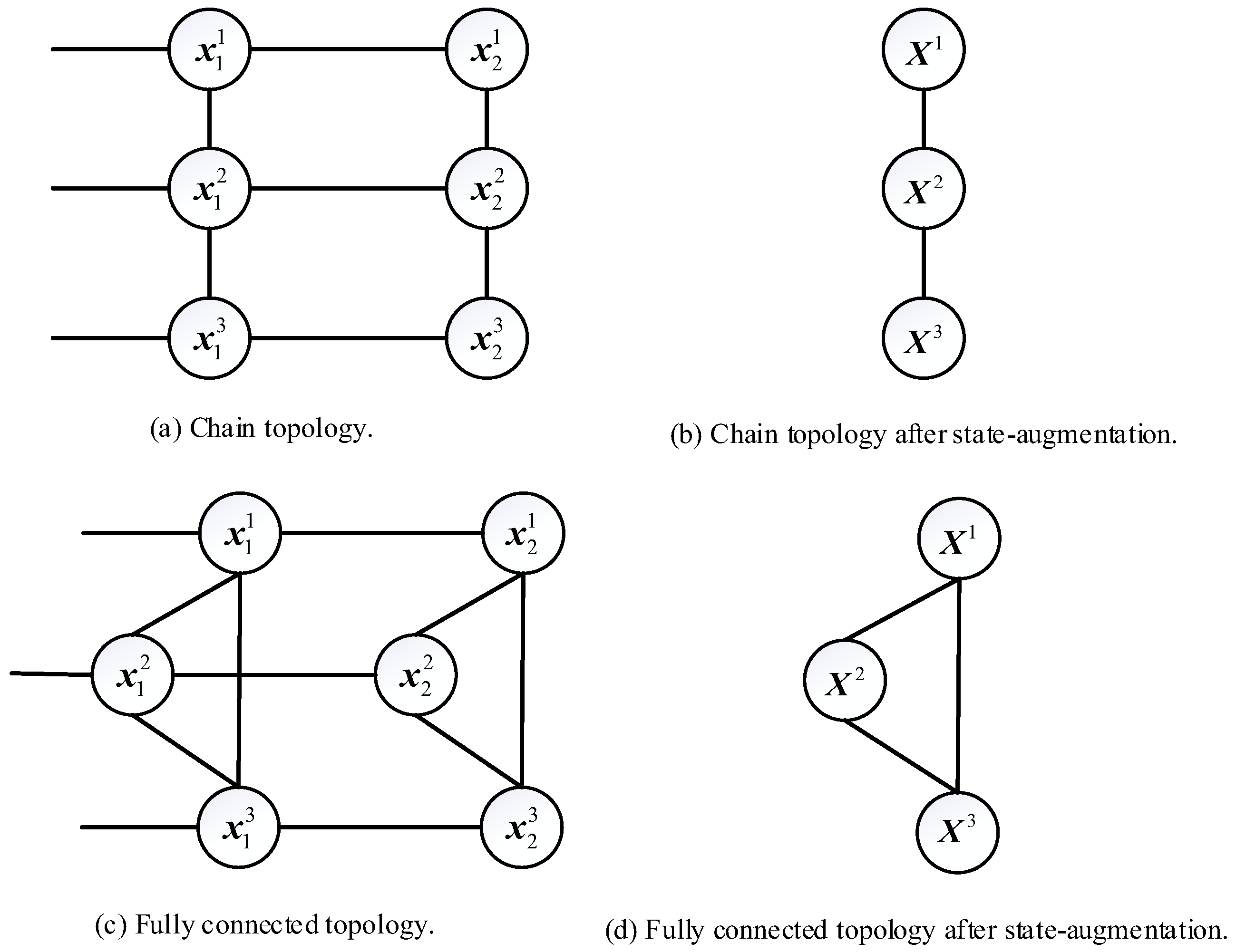
5.1. Motivation

As we can see, the BP-based CL is generally recursive along time, and iterative at each time instant for the existence of loops in the factor graph. That is to say, the BP algorithm only accounts for the loops existing at one time instant and neglects the loops across time. This approximation brings to the BP-based CL the recursion property, conciseness in procedures, and straightforwardness in implementation. However, the resulting error caused by neglecting the loops across time will accumulate and degrade the accuracy of localization. Completely eliminating this approximation needs to consider all loops from the initial time to the current time, which is computationally infeasible, not to mention the tremendous communication cost. To deal with this problem, we propose to allow message backward passing in the factor graph via state augmentation.

To consider the loops across time, the messages in BP need to propagate in both forward and backward directions. However, due to the complexity of the factor graph structure, it is difficult to find a suitable message propagation order, i.e., message propagation schedule [27]. Fortunately, for mobile agent networks, all agents naturally have their historical states, which allow us to realize message backward propagation by state augmentation. The idea is similar to the fixed-lag smoother [31]. They both utilize state augmentation. However, the optimal fixed-lag smoother only cares about the estimation of a previous state (at a fixed-lag time) and cannot improve the state estimation at the current time. The augmented state BP (AS-BP) aims to improve the state estimation at current time and can intuitively achieve this goal by considering the loops across time. We use the following example to show how the state augmentation accounts for the loops across time.

Example 1.

Consider two different agent network topologies, i.e., a chain topology and a fully connected topology, as shown in Figure 2. For brevity, boxes representing the factor nodes are omitted in the factor graphs shown in Figure 2 and we know each link connecting two variable nodes acts as a factor node. Figure 2b,d show the factor graphs after state augmentation according to Figure 2a and Figure 2c, respectively. For the chain topology shown in Figure 2a, the factor graph after state augmentation is loop-free as shown in Figure 2b, and thus an accurate conditional marginal pdf can be obtained without any iteration. For the fully connected topology shown in Figure 2c, loops both at one time instant and across time exist. After stat-augmentation shown in Figure 2d, only one loop is left. Iterations are still needed in the BP for Figure 2d since there is still a loop. However, it is intuitive that the BP on the augmented state (shown in Figure 2d) outperforms the BP acting on the fact graph shown in Figure 2c since the number of loops is significantly reduced.

5.2. Augmented State BP (AS-BP) Algorithm

For the ease of presentation, we consider to augment states at two successive times. That is to say, we only consider the AS-BP with 1-step retrodiction. The n-step ($n\ge 2$) algorithms can be implemented according to readers’ concrete applications. Let ${\mathit{X}}_{k+2}^i={[{({\mathit{x}}_{k+2}^i)}^{\mathrm{T}},{({\mathit{x}}_{k+1}^i)}^{\mathrm{T}}]}^{\mathrm{T}}$ and ${\mathit{Z}}_{k+2}^i={[{({\mathit{z}}_{k+2}^i)}^{\mathrm{T}},{({\mathit{z}}_{k+1}^i)}^{\mathrm{T}}]}^{\mathrm{T}}$. For each agent $i\in \mathcal{A}$, the prediction message $m_{\to k+2}({\mathit{X}}_{k+2}^i)$ is given by

$$m_{\to k+2}({\mathit{X}}_{k+2}^i)\propto \int f({\mathit{Z}}_{k+2}^i|{\mathit{X}}_{k+2}^i,{\mathit{x}}_k^i)f({\mathit{X}}_{k+2}^i|{\mathit{x}}_k^i)b^p({\mathit{x}}_k^i)d{\mathit{x}}_k^i$$

(22)

From Equations (1) and (2), we have

$$m_{\to k+2}({\mathit{X}}_{k+2}^i)\propto \mathcal{N}({\mathit{X}}_{k+2}^i,{\hat{\mathit{X}}}_{k+2|k}^{\mathit{m},i},{\mathit{P}}_{k+2|k}^{\mathit{m},i})$$

(23)

The calculation of the message $m_{\to k+2}({\mathit{X}}_{k+2}^i)$ involves prediction and update. Note that by state augmentation, the measurements used in the update involve not only ${\mathit{z}}_{k+2}^i$ but also ${\mathit{z}}_{k+1}^i$. The prediction is

$${\hat{\mathit{X}}}_{k+2|k}^{p,i}={\mathit{F}}_k^{p,i}{\hat{\mathit{X}}}_{k|k}^i$$

(24)

$${\mathit{P}}_{k+2|k}^{p,i}={\mathit{F}}_k^{p,i}{\mathit{P}}_{k|k}^i{({\mathit{F}}_k^{p,i})}^{\mathrm{T}}+{\mathit{G}}_k^{p,i}{\mathit{Q}}_k^{p,i}{({\mathit{G}}_k^{p,i})}^{\mathrm{T}}$$

(25)

where

$$\begin{array}{l}{\mathit{F}}_k^{p,i}=\left[\begin{array}{cc}{\mathit{F}}_{k+1}^i{\mathit{F}}_k^i& 0\\ {\mathit{F}}_k^i& 0\end{array}\right]\\ {\mathit{G}}_k^{p,i}=\left[\begin{array}{cc}{\mathit{G}}_{k+1}^i& {\mathit{F}}_{k+1}^i{\mathit{G}}_k^i\\ 0& {\mathit{G}}_k^i\end{array}\right]\\ {\mathit{Q}}_k^{p,i}=\mathrm{diag}({\mathit{Q}}_{k+1}^i,{\mathit{Q}}_k^i)\end{array}$$

and the update is

$${\hat{\mathit{X}}}_{k+2|k}^{\mathit{m},i}={\hat{\mathit{X}}}_{k+2|k}^{p,i}+{\mathit{W}}_{k+2}^i({\mathit{Z}}_{k+2}^i-{\hat{\mathit{Z}}}_{k+2}^i)$$

(26)

$${\mathit{P}}_{k+2|k}^{\mathit{m},i}={\mathit{P}}_{k+2|k}^{p,i}-{\mathit{W}}_{k+2}^i{\mathit{S}}_{k+2}^i{({\mathit{W}}_{k+2}^i)}^{\mathrm{T}}$$

(27)

where

$$\begin{array}{l}{\hat{\mathit{Z}}}_{k+2}^i={\mathit{H}}_{k+2}^{{\mathit{m}}_1,i}{\hat{\mathit{X}}}_{k+2|k}^{p,i}-{\mathit{H}}_{k+2}^{{\mathit{m}}_2,i}{\hat{\mathit{X}}}_{k|k}^i\\ {\mathit{S}}_{k+2}^i={\mathit{R}}_{k+2}^{\mathit{m},i}+{\mathit{H}}_{k+2}^{{\mathit{m}}_1,i}{\mathit{P}}_{k+2|k}^{p,i}{({\mathit{H}}_{k+2}^{{\mathit{m}}_1,i})}^{\mathrm{T}}+{\mathit{H}}_{k+2}^{{\mathit{m}}_2,i}{\mathit{P}}_{k|k}^i{({\mathit{H}}_{k+2}^{{\mathit{m}}_2,i})}^{\mathrm{T}}\\ -{\mathit{H}}_{k+2}^{{\mathit{m}}_1,i}{\mathit{F}}_k^{p,i}{\mathit{P}}_{k|k}^i{({\mathit{H}}_{k+2}^{{\mathit{m}}_2,i})}^{\mathrm{T}}-{\mathit{H}}_{k+2}^{{\mathit{m}}_2,i}{\mathit{P}}_{k|k}^i{({\mathit{F}}_k^{p,i})}^{\mathrm{T}}{({\mathit{H}}_{k+2}^{{\mathit{m}}_1,i})}^{\mathrm{T}}\\ {\mathit{W}}_{k+2}^i=({\mathit{P}}_{k+2|k}^{p,i}{({\mathit{H}}_{k+2}^{{\mathit{m}}_1,i})}^{\mathrm{T}}-{\mathit{F}}_k^{p,i}{\mathit{P}}_{k|k}^i{({\mathit{H}}_{k+2}^{{\mathit{m}}_2,i})}^{\mathrm{T}}){({\mathit{S}}_{k+2}^i)}^{-1}\end{array}$$

with ${\mathit{H}}_{k+2}^{{\mathit{m}}_1,i}=\left[\begin{array}{cc}{\mathit{H}}_{k+2}^i& -{\mathit{H}}_{k+2}^i\\ 0& {\mathit{H}}_{k+1}^i\end{array}\right]$, ${\mathit{H}}_{k+2}^{{\mathit{m}}_2,i}=\left[\begin{array}{cc}0& 0\\ {\mathit{H}}_{k+1}^i& 0\end{array}\right]$ and ${\mathit{R}}_{k+2}^{\mathit{m},i}=\mathrm{diag}({\mathit{R}}_{k+1}^i,{\mathit{R}}_k^i)$. Then, it comes to calculate the message $n_{j\to i}^p({\mathit{X}}_{k+2}^j)$. Following Equations (20) and (21), we have

$$n_{j\to i}^p({\mathit{X}}_{k+2}^j)=\int m_{\to k+2}({\mathit{X}}_{k+2}^j){\displaystyle \prod }_{l\in {\mathcal{N}}_{k+2}^j\backslash i}f({\mathit{Z}}_{k+2}^{l,j}|{\mathit{X}}_{k+2}^l,{\mathit{X}}_{k+2}^j)n_{l\to j}^{p-1}({\mathit{X}}_{k+2}^l)d{\mathit{X}}_{k+2}^l$$

(28)

where ${\mathit{Z}}_{k+2}^{l,j}={[{({\mathit{z}}_{k+2}^{l,j})}^{\mathrm{T}},{({\mathit{z}}_{k+2}^{j,l})}^{\mathrm{T}},{({\mathit{z}}_{k+1}^{l,j})}^{\mathrm{T}},{({\mathit{z}}_{k+1}^{j,l})}^{\mathrm{T}}]}^{\mathrm{T}}$ and ${\mathcal{N}}_{k+2}^j={\mathcal{N}}_{j,k+2}\cup {\mathcal{N}}_{j,k+1}$. Equation (28) can be calculated by performing the update step of Kalman filter and is given by

$$n_{j\to i}^p({\mathit{X}}_{k+2}^j)\propto \mathcal{N}({\mathit{X}}_{k+2}^j;{\hat{\mathit{X}}}_{k+2}^{p,ji},{\mathit{P}}_{k+2}^{p,ji})$$

(29)

where

$${\hat{\mathit{X}}}_{k+2}^{p,ji}={\hat{\mathit{X}}}_{k+2|k}^{\mathit{m},j}+{\mathit{W}}_{k+2}^{p,ji}({\mathit{Z}}_{k+2}^{ji}-{\hat{\mathit{Z}}}_{k+2}^{p,ji})$$

(30)

$${\mathit{P}}_{k+2}^{p,ji}={\mathit{P}}_{k+2|k}^{\mathit{m},j}-{\mathit{W}}_{k+2}^{p,ji}{\mathit{S}}_{k+2}^{p,ji}{({\mathit{W}}_{k+2}^{p,ji})}^{\mathrm{T}}$$

(31)

and

$$\begin{array}{l}{\mathit{Z}}_{k+2}^{ji}={\left[{\left\{{({\mathit{Z}}_{k+2}^{j,l})}^{\mathrm{T}}\right\}}_{l\in {\mathcal{N}}_{k+2}^j\backslash i}\right]}^{\mathrm{T}}\\ {\hat{\mathit{Z}}}_{k+2}^{p,ji}={\left[{\left\{{({\mathit{H}}_{k+2}^{jl}({\hat{\mathit{X}}}_{k+2}^{p-1,lj}-{\hat{\mathit{X}}}_{k+2|k}^{m,j}))}^{\mathrm{T}}\right\}}_{l\in {\mathcal{N}}_{k+2}^j\backslash i}\right]}^{\mathrm{T}}\\ {\mathit{R}}_{k+2}^{n,ji}=\mathrm{diag}({\{{\mathit{R}}_{k+2}^{jl}+{\mathit{H}}_{k+2}^{jl}{\mathit{P}}_{k+2}^{p-1,lj}{({\mathit{H}}_{k+2}^{jl})}^{\mathrm{T}}\}}_{l\in {\mathcal{N}}_{k+2}^j\backslash i})\\ {\mathit{R}}_{k+2}^{jl}=\mathrm{diag}({\mathit{R}}_{k+2}^{j,l},{\mathit{R}}_{k+2}^{l,j},{\mathit{R}}_{k+1}^{j,l},{\mathit{R}}_{k+1}^{l,j})\\ {\mathit{S}}_{k+2}^{p,ji}={\mathit{H}}_{k+2}^{n,ji}{\mathit{P}}_{k+2|k}^{m,j}{({\mathit{H}}_{k+2}^{n,ji})}^{\mathrm{T}}+{\mathit{R}}_{k+2}^{n,ji}\\ {\mathit{W}}_{k+2}^{p,ji}={\mathit{P}}_{k+2|k}^{m,j}{({\mathit{H}}_{k+2}^{n,ji})}^{\mathrm{T}}{({\mathit{S}}_{k+2}^{p,ji})}^{-1}\\ {\mathit{H}}_{k+2}^{n,ji}={\left[{\left\{{({\mathit{H}}_{k+2}^{jl})}^{\mathrm{T}}\right\}}_{l\in {\mathcal{N}}_{k+2}^j\backslash i}\right]}^{\mathrm{T}}\\ {\mathit{H}}_{k+2}^{jl}=\left[\begin{array}{cc}{\mathit{H}}_{k+2}^{j,l}& \mathbf{0}\\ -{\mathit{H}}_{k+2}^{l,j}& \mathbf{0}\\ \mathbf{0}& {\mathit{H}}_{k+1}^{j,l}\\ \mathbf{0}& -{\mathit{H}}_{k+1}^{l,j}\end{array}\right]\end{array}$$

For simplicity of notation, we use ${\left\{{(a^l)}^{\mathrm{T}}\right\}}_{l\in \mathcal{A}}$ to denote stacking all vectors $a^l,l=1,\dots ,|\mathcal{A}|$ into a row vector with a fixed index order of elements in set $\mathcal{A}$, where $|\mathcal{A}|$ is the cardinality of the set $\mathcal{A}$.

The initial message $n_{j\to i}^0({\mathit{X}}_{k+2}^j)$ is $m_{\to k+2}({\mathit{X}}_{k+2}^j)$. Since Equation (18) is analogous to Equation (21), the belief $b^p({\mathit{X}}_{k+2}^i)$, which is approximately the conditional marginal pdf $f({\mathit{X}}_{k+2}^i|{\mathit{Z}}_{1:k+2})$, can be calculated in a similar way to the message $n_{j\to i}^p({\mathit{X}}_{k+2}^j)$. The overall algorithm is given in Algorithm 1.

Algorithm 1 AS-BP algorithm.

Start with ${\hat{\mathit{x}}}_{0|0}^i={\overline{\mathit{x}}}_0^i$, ${\mathit{P}}_{0|0}^i={\mathit{P}}_0^i$, and compute at each agent $i$: Step 1. Calculate the prediction message $m_{\to k}({\mathit{X}}_k^i)$ as in Equations (23)–(27). Step 2. Calculate the belief $b^p({\mathit{X}}_k^i)$:     1: for $p^{\prime }=1\mathrm{to}p$ do     2: Calculate the message $n_{i\to j}^{p^{\prime }-1}({\mathit{X}}_k^i)$ as in Equations (29)–(31) and its initial value $n_{i\to j}^0({\mathit{X}}_k^i)$ is set to $m_{\to k}({\mathit{X}}_k^i)$.     3: Send $n_{i\to j}^{p^{\prime }-1}({\mathit{X}}_k^i)$ and $z_k^{i,j}$ to its neighbor agent $j$.     4: Receive $n_{j\to i}^{p^{\prime }-1}({\mathit{X}}_k^j)$ and $z_k^{j,i}$, $j\in {\mathcal{N}}_k^i$.     5: Calculate the belief $b^{p^{\prime }}({\mathit{X}}_k^i)$ as in Equations (29)–(31) but it is a little different, that is $l\in {\mathcal{N}}_k^i$.     6: end for

5.3. Computation and Communication Overhead

From Equations (18)–(21), it can be seen that the BP algorithm, for each agent $i$ in each iteration, needs to calculate the belief $b({\mathit{x}}_k^i)$ and the outgoing message $n_{i\to j}^p({\mathit{x}}_k^i)$ based on the incoming messages $m_{j\to i}^p({\mathit{x}}_k^i)$ from all neighboring agents $j\in {\mathcal{A}}_{i,k}$ and its own prediction message $m_{\to k}({\mathit{x}}_k^i)$. The computational complexity of the BP algorithm increases linearly with the scale of the network. Our proposed algorithm utilizes state augmentation to realize messages backward propagation, which capably retains the excellent characteristics of the BP algorithm. However, due to the use of state augmentation, the computational cost inevitably increases. Compared with the BP algorithm, the computational cost of the proposed algorithm increases linearly with the number of retrodiction steps. By using state augmentation, the computational time of AS-BP increases along with the retrodiction step compared with original BP. The computational complexity is generally $O({(r{d}_z)}^3)$, where $d_z^{}$ is the dimension of relative measurements and $r$ is the number of retrodiction steps, since matrix inverse is involved in Equations (30) and (31). This nonlinear increase of computation can be avoided by a sequential (or recursive) implementation of the update of the Kalman filter due to the uncorrelated assumption of relative measurement noises [32]. With such an implementation, the computational time of AS-BP increases linearly with the retrodiction step, since it is equivalent to say $r$ times of filtering of original BP are needed in the AS-BP. On the other hand, if the batch form of update in Equations (30) and (31) is directly used in the implementation of AS-BP. The computational time still shows nearly linear increase along with the retrodiction step $r$, when $r$ is relatively small. This is due to the fact that the nonlinear part of the matrix inverse is not dominating in the whole filtering procedure.

For the communication cost, since Gaussian BP is used in this paper, the data that each agent $i$ needs to transmit to its neighbor $j$ are only the first two moments of the outgoing message $n_{i\to j}^p({\mathit{x}}_k^i)$ and the relative measurements between them. The communication cost of the proposed algorithm is increased by $(r^2-1)d^2+(r-1)d$ compared with the original BP algorithm, where $d$ is the dimension of the agent state. The BP algorithm requires peer-to-peer communication, which has high communication requirements. To solve this problem, the belief can be transmitted instead of messages [10,21]. In this way, the agent can perform broadcast communication, which greatly reduces the communication requirements. This is beyond the scope of this paper and thus is not discussed in detail here.

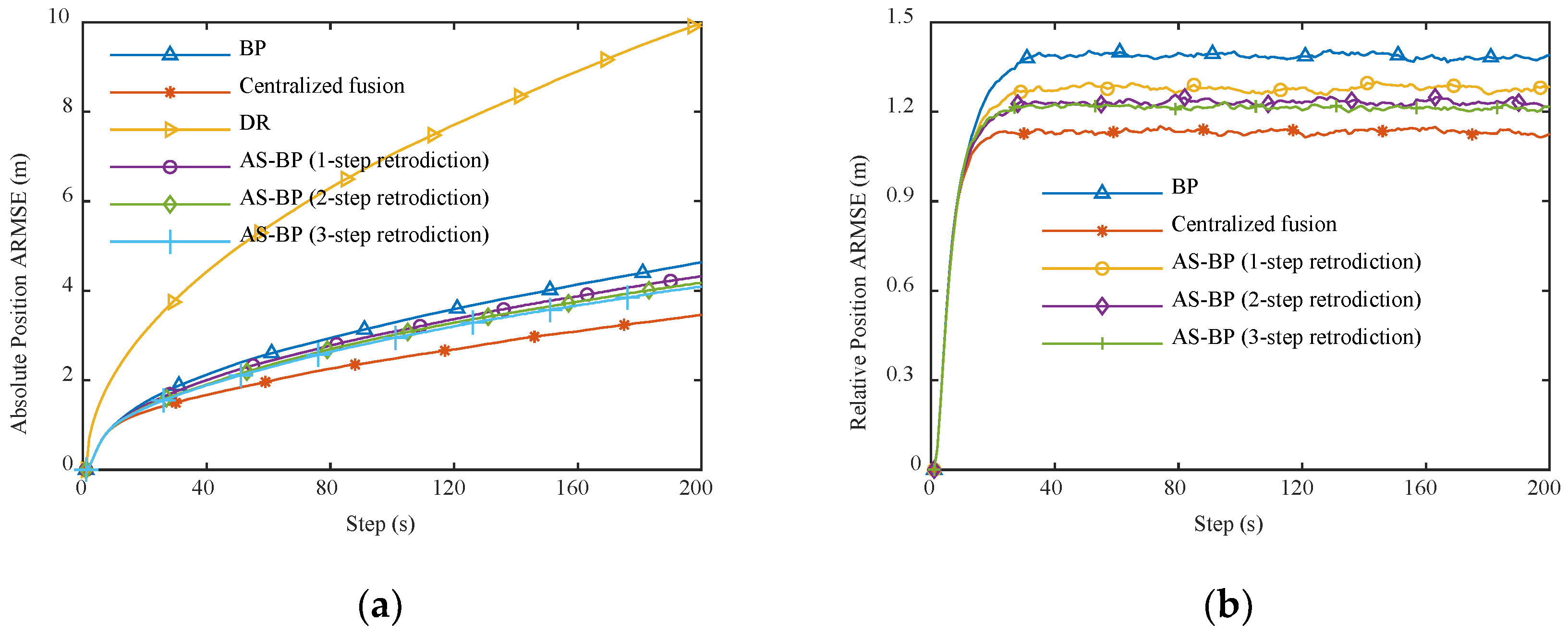
6. Illustrative Examples

Two scenarios of CL are simulated to verify the performance of our proposed AS-BP algorithm. Both scenarios use the same motion agents but different network topologies, including a chain and a full connected topology. The network contains $N=9$ agents and each agent moves according to a nearly constant velocity model in a two-dimensional plane. The dynamic model of each agent is formulated by Equation (1) with

$$\begin{array}{l}{\mathit{F}}_k^i=\mathrm{diag}(\mathit{F},\mathit{F}),{\mathit{G}}_k^i=\mathrm{diag}(\mathit{G},\mathit{G})\\ \mathit{F}=\left[\begin{array}{cc}1& T\\ 0& 1\end{array}\right],\mathit{G}=\left[\begin{array}{c}{T}^2/2\\ T\end{array}\right]\\ {\mathit{w}}_k^i\sim \mathcal{N}(0,\mathit{Q})\end{array}$$

(32)

where the time interval $T=1\mathrm{s}$ and $\mathit{Q}=\mathrm{diag}(0.01{\mathrm{m}}^2{/\mathrm{s}}^4,0.01{\mathrm{m}}^2{/\mathrm{s}}^4)$.

In the simulation, the initial state ${\mathit{x}}_0^i$ is distributed as $\mathcal{N}({\mathit{x}}_0^i;{\overline{\mathit{x}}}_0^i,p_0^i)$, where ${\overline{\mathit{x}}}_0^i$ is set as

$$\begin{array}{l}{\overline{\mathit{x}}}_0^1={[0\mathrm{m},20\mathrm{m}/\mathrm{s},400\mathrm{m},20\mathrm{m}/\mathrm{s}]}^{\mathrm{T}},{\overline{\mathit{x}}}_0^2={[100\mathrm{m},20\mathrm{m}/\mathrm{s},400\mathrm{m},20\mathrm{m}/\mathrm{s}]}^{\mathrm{T}}\\ {\overline{\mathit{x}}}_0^3={[200\mathrm{m},20\mathrm{m}/\mathrm{s},400\mathrm{m},20\mathrm{m}/\mathrm{s}]}^{\mathrm{T}},{\overline{\mathit{x}}}_0^4={[300\mathrm{m},20\mathrm{m}/\mathrm{s},400\mathrm{m},20\mathrm{m}/\mathrm{s}]}^{\mathrm{T}}\\ {\overline{\mathit{x}}}_0^5={[400\mathrm{m},20\mathrm{m}/\mathrm{s},400\mathrm{m},20\mathrm{m}/\mathrm{s}]}^{\mathrm{T}},{\overline{\mathit{x}}}_0^6={[400\mathrm{m},20\mathrm{m}/\mathrm{s},300\mathrm{m},20\mathrm{m}/\mathrm{s}]}^{\mathrm{T}}\\ {\overline{\mathit{x}}}_0^7={[400\mathrm{m},20\mathrm{m}/\mathrm{s},200\mathrm{m},20\mathrm{m}/\mathrm{s}]}^{\mathrm{T}},{\overline{\mathit{x}}}_0^8={[400\mathrm{m},20\mathrm{m}/\mathrm{s},100\mathrm{m},20\mathrm{m}/\mathrm{s}]}^{\mathrm{T}}\\ {\overline{\mathit{x}}}_0^9={[400\mathrm{m},20\mathrm{m}/\mathrm{s},0\mathrm{m},20\mathrm{m}/\mathrm{s}]}^{\mathrm{T}}\end{array}$$

and the covariance ${\mathit{P}}_0^i=\mathrm{diag}({0.002}^2{\mathrm{m}}^2,{0.002}^2{\mathrm{m}}^2{/\mathrm{s}}^2,{0.002}^2{\mathrm{m}}^2,{0.002}^2{\mathrm{m}}^2{/\mathrm{s}}^2)$. The internal measurements model and the relative measurement model are as in Equations (2) and (3) with ${\mathit{H}}_k^{i,j}={\mathit{H}}_k^i=\left[\begin{array}{cccc}1& 0& 0& 0\\ 0& 0& 1& 0\end{array}\right]$, ${\mathit{R}}_k^i=\mathrm{diag}(0.25{\mathrm{m}}^2,0.25{\mathrm{m}}^2)$ and ${\mathit{R}}_k^{i,j}=\mathrm{diag}(4{\mathrm{m}}^2,4{\mathrm{m}}^2)$, where $i=1,2,\dots ,N$ and $j\in {\mathcal{N}}_{i,k}$. We use the average root mean square error (ARMSE) over all agents to compare different algorithms

$$\mathrm{ARMSE}=\frac{1}{N}{\displaystyle \sum }_{i=1}^N\mathrm{RMSE}({\mathit{x}}_k^i)$$

(33)

The absolute position refers to the position in the fixed global coordinate system, and the relative position refers to a moving coordinate system taking the position of agent 1 as the origin. For the chain topology, the number of iterations is set to be 3 for both the AS-BP and the BP. For the fully connected scenario, it is set to be 5. All simulations have performed a total of 5000 Monte Carlo runs. The simulation results are shown in Figure 3 and Figure 4.

In all simulations, the AS-BP algorithm and the BP algorithm show better absolute localization accuracy than DR. This reflects the advantage of CL in which the error accumulation of IMU can be effectively alleviated through cooperation. In the chain topology scenario, the AS-BP algorithm has better absolute localization accuracy and relative localization accuracy than the BP algorithm. As the number of retrodiction steps increases, the localization accuracy of the AS-BP gradually improves. This is because the AS-BP performs messages backward propagation by using state augmentation, which effectively increases the available information of agents and thereby reduces the accumulation of errors caused by the approximation of beliefs. In the scenario of chain topology, as the steps of retrodiction increase, the number of loops in the factor graph approaches to zero and the performance of the proposed algorithm approaches to the one of the centralized fusion. In the fully connected topology scenario, the BP algorithm and the AS-BP algorithm have a relative localization accuracy similar to that of the centralized fusion. This is because the entire network has adequate information from relative measurements and can achieve better performance. However, since the amount of absolute position information has not increased, the absolute localization accuracy of the BP algorithm and the AS-BP algorithm are still lower than that of the centralized fusion. On the other hand, due to the use of state augmentation, the AS-BP algorithm has a higher absolute localization accuracy than the BP algorithm. However, note that, unlike in the chain topology, in the fully connected topology scenario, the use of state augmentation can only reduce the loops in the factor graph but cannot completely eliminate them. Therefore, in this case, the AS-BP algorithm can only improve the performance of the BP algorithm, but cannot achieve the centralized fusion. More loops in the fully connected scenario exist than in the chain topology scenario. Thus, accumulation of errors caused by the belief approximation increases more severely in the fully connected scenario than in the chain scenario, that is why the absolute localization accuracy of the BP algorithm and the AS-BP algorithm in the fully connected topology scenario is lower than that in the chain topology scenario.

The relative computation time of the AS-BP algorithm and the BP algorithm in Matlab are provided in

Table 1. Relative computation time for the chain topology.

BP	AS-BP (1-Step Retrodiction)	AS-BP (2-Step Retrodiction)	AS-BP (3-Step Retrodiction)
1.0000	1.6697	2.2094	2.8575

and

Table 2. Relative computation time for the fully connected topology.

BP	AS-BP (1-Step Retrodiction)	AS-BP (2-Step Retrodiction)	AS-BP (3-Step Retrodiction)
1.0000	2.1122	3.7309	5.4305

. It can be seen that the computational cost of the AS-BP algorithm increases almost linearly with the increase of the retrodiction steps.

7. Conclusions

In this paper, an augmented state BP algorithm for mobile agent networks has been proposed. Compared with the existing BP algorithms, AS-BP further considers the across time loops in the factor graph. By state augmentation, the messages in the factor graph can be backward propagated, which reduces the number of loops in the factor graph, increases the available information of the agent, and improves the localization accuracy of the agent. When the network topology has no loops, AS-BP can obtain the optimal estimation. Otherwise, AS-BP can only obtain approximate estimations. However, the large reduction of loops allows AS-BP to still have higher estimation accuracy than the original BP. AS-BP can be directly combined with nonlinear algorithms to deal with nonlinear measurement scenarios. Compared with the original BP, AS-BP has higher computational and communicational costs, so we suggest using limited steps of retrodiction. Experimental results demonstrate the performance of our algorithm. In addition, this paper has reformulated the CL problem in a more general form and gives its corresponding centralized fusion algorithm. Future work includes further reducing the computation and communication overhead of the algorithm.

References

1. Liu, K.; Lim, H.B.; Frazzoli, E.; Ji, H.; Lee, V.C.S. Improving positioning accuracy using GPS pseudorange measurements for cooperative vehicular localization. IEEE Trans. Veh. Technol. 2014, 63, 2544–2556. [Google Scholar] [CrossRef]
2. Sun, G.; Zhou, R.; Xu, K.; Weng, Z.; Zhang, Y.; Dong, Z.; Wang, Y. Cooperative formation control of multiple aerial vehicles based on guidance route in a complex task environment. Chin. J. Aeronaut. 2020, 33, 701–720. [Google Scholar] [CrossRef]
3. Ahmad, A.; Lawless, G.; Lima, P. An online scalable approach to unified multirobot cooperative localization and object tracking. IEEE Trans. Robot. 2017, 33, 1184–1199. [Google Scholar] [CrossRef]
4. Roman, R.C.; Precup, R.E.G.; Petriu, E.M. Hybrid data-driven fuzzy active disturbance rejection control for tower crane systems. Eur. J. Control 2021, 58, 373–387. [Google Scholar] [CrossRef]
5. Chi, R.H.; Li, H.Y.; Shen, D.; Hou, Z.; Huang, B. Enhanced P-type Control: Indirect Adaptive Learning from Set-point Updates. IEEE Trans. Autom. Control 2022. [Google Scholar] [CrossRef]
6. Paull, L.; Saeedi, S.; Seto, M.; Li, H. AUV navigation and localization: A review. IEEE J. Ocean. Eng. 2014, 39, 1184–1199. [Google Scholar] [CrossRef]
7. Roumeliotis, S.I.; Bekey, G.A. Distributed multirobot localization. IEEE Trans. Robot. Autom. 2002, 18, 781–795. [Google Scholar] [CrossRef] [Green Version]
8. Shen, Y.; Wymeersch, H.; Win, M.Z. Fundamental limits of wideband localization-part II: Cooperative networks. IEEE Trans. Inf. Theory 2010, 56, 4981–5000. [Google Scholar] [CrossRef] [Green Version]
9. Zhai, G.; Zhang, J.; Zhou, Z. Coordinated target localization base on pseudo measurement for clustered space robot. Chin. J. Aeronaut. 2013, 26, 1524–1533. [Google Scholar] [CrossRef] [Green Version]
10. Wymeersch, H.; Lien, J.; Win, M.Z. Cooperative localization in wireless networks. Proc. IEEE 2009, 97, 427–450. [Google Scholar] [CrossRef]
11. Nguyen, T.V.; Jeong, Y.; Shin, H.; Win, M.Z. Least square cooperative localization. IEEE Trans. Veh. Technol. 2015, 64, 1318–1330. [Google Scholar] [CrossRef]
12. Ouyang, R.W.; Wong, A.K.S.; Lea, C.T. Received signal strength-based wireless localization via semidefinite programming: Noncooperative and cooperative schemes. IEEE Trans. Veh. Technol. 2010, 59, 1307–1318. [Google Scholar] [CrossRef]
13. Vaghefi, R.M.; Buehrer, R.M. Cooperative joint synchronization and localization in wireless sensor networks. IEEE Trans. Signal Process. 2015, 63, 3615–3627. [Google Scholar] [CrossRef]
14. Pearl, J. Probabilistic Reasoning in Intelligent Systems: Networks of Plausible Inference; Morgan Kaufmann: San Mateo, CA, USA, 1988. [Google Scholar]
15. Wainwright, M.J.; Jaakkola, T.S.; Willsky, A.S. Tree-based reparameterization framework for analysis of sum-product and related algorithms. IEEE Trans. Inf. Theory 2003, 49, 1120–1146. [Google Scholar] [CrossRef] [Green Version]
16. Su, Q.; Wu, Y.C. Convergence analysis of the variance in Gaussian belief propagation. IEEE Trans. Veh. Technol. 2014, 62, 5119–5131. [Google Scholar] [CrossRef] [Green Version]
17. Yuan, W.; Wu, N.; Etzlinger, B.; Wang, H.; Kuang, J. Cooperative joint localization and clock synchronization based on Gaussian message passing in asynchronous wireless networks. IEEE Trans. Veh. Technol. 2016, 65, 7258–7273. [Google Scholar] [CrossRef] [Green Version]
18. Sudderth, E.B.; Ihler, A.T.; Freeman, W.T.; Willsky, A.S. Nonparametric belief propagation. In Proceedings of the 2003 IEEE Computer Society Conference on Computer Vision and Pattern Recognition, Madison, WI, USA, 18–20 June 2003; pp. I-605–I-612. [Google Scholar]
19. Ihler, A.T.; Fisher, J.W.; Moses, R.L.; Willsky, A.S. Nonparametric belief propagation for self-localization of sensor networks. IEEE J. Sel. Areas Commun. 2005, 23, 809–819. [Google Scholar] [CrossRef] [Green Version]
20. Ihler, A.T.; Sudderth, E.B.; Freeman, W.T.; Willsky, A. Efficient multiscale sampling from products of Gaussian mixtures. In Proceedings of the 17th Annual Conference on Neural Information Processing Systems (NIPS), Vancouver, BC, Canada, 13–18 December 2004; pp. 1–8. [Google Scholar]
21. Savic, V.; Zazo, S. Reducing communication overhead for cooperative localization using nonparametric belief propagation. IEEE Wirel. Commun. Lett. 2012, 1, 308–311. [Google Scholar] [CrossRef] [Green Version]
22. Li, Y.; Wang, Y.; Yu, W.; Guan, X. Multiple autonomous underwater vehicle cooperative localization in anchor-free environments. IEEE J. Ocean. Eng. 2019, 44, 895–911. [Google Scholar] [CrossRef]
23. Garcia-Fernandez, A.F.; Svensson, L.; Sarkka, S. Cooperative localization using posterior linearization belief propagation. IEEE Trans. Veh. Technol. 2018, 67, 832–836. [Google Scholar] [CrossRef]
24. Meyer, F.; Hlinka, O.; Hlawatsch, F. Sigma point belief propagation. IEEE Signal Process. Lett. 2014, 21, 145–149. [Google Scholar] [CrossRef] [Green Version]
25. Li, S.; Hedley, M.; Collings, I.B. New efficient indoor cooperative localization algorithm with empirical ranging error model. IEEE J. Sel. Areas Commun. 2015, 33, 1407–1417. [Google Scholar] [CrossRef]
26. Georges, H.M.; Xiao, Z.; Wang, D. Hybrid cooperative vehicle positioning using distributed randomized sigma point belief propagation on non-Gaussian noise distribution. IEEE Sens. J. 2016, 16, 7803–7813. [Google Scholar] [CrossRef]
27. Kschischang, F.R.; Frey, B.J.; Loeliger, H.A. Factor graphs and the sum-product algorithm. IEEE Trans. Inf. Theory 2001, 47, 498–519. [Google Scholar] [CrossRef] [Green Version]
28. Barooah, P.; Russell, W.J.; Hespanha, J.P. Approximate distributed Kalman filtering for cooperative multi-agent localization. In Proceedings of the 6th IEEE International Conference on Distributed Computing in Sensor Systems, Santa Barbara, CA, USA, 21–23 June 2010; pp. 102–115. [Google Scholar]
29. Li, X.R.; Zhu, Y.M.; Wang, J.; Han, C. Optimal linear estimation fusion—Part I: Unified fusion rules. IEEE Trans. Inf. Theory 2003, 49, 2192–2208. [Google Scholar] [CrossRef]
30. Bar-Shalom, Y.; Li, X.R.; Kirubarajan, T. Estimation with Applications to Tracking and Navigation: Theory, Algorithms and Software; Wiley: New York, NY, USA, 2001. [Google Scholar]
31. Gao, Y.X.; Li, X.R. Optimal linear fusion of smoothed state estimates. IEEE Trans. Aerosp. Electron. Syst. 2012, 48, 1236–1248. [Google Scholar]
32. Li, X.R. Recursibility and optimal linear estimation and filtering. In Proceedings of the 43rd IEEE Conference on Decision and Control, Nassau, The Bahamas, 14–17 December 2004; pp. 1761–1766. [Google Scholar]
Figure 1. Factor graph of the joint pdf f ( X 0 : k | Z 1 : k ) . For brevity, we only drew the part related to x k 1 in detail, and the factor nodes are represented by abbreviations, where f k i = f ( z k i | x k i ,   x k 1 i ) f ( x k i | x k 1 i ) and f k i , j = f ( z k i ,   j ,   z k j ,   i | x k i ,   x k j ) . The arrows indicate the directions of message propagation.
Electronics 11 01959 g001
Figure 2. Factor graphs.
Electronics 11 01959 g002
Figure 3. Absolute and relative position RMSEs in chain topology. (a) Absolute position RMSE. (b) Relative position RMSE.
Electronics 11 01959 g003
Figure 4. Absolute and relative position RMSEs in fully connected topology. (a) Absolute position RMSE. (b) Relative position RMSE.
Electronics 11 01959 g004