Article

Identification of Secondary Breast Cancer in Vital Organs through the Integration of Machine Learning and Microarrays

1
Department of Information Systems, University of Management and Technology, Lahore 54770, Pakistan
2
Department of Information Technology, The University of Haripur, Haripur 22620, Pakistan
3
Department of Software and Communications Engineering, Hongik University, Sejong 30016, Korea
4
Department of Computer Science, College of Computer and Information Sciences, King Saud University, Riyadh 11633, Saudi Arabia
5
Management and Organizational Behaviour Business School, University for the Creative Arts, Epsom KT18 5BE, UK
*
Author to whom correspondence should be addressed.
Electronics 2022, 11(12), 1879; https://doi.org/10.3390/electronics11121879
Submission received: 27 April 2022 / Revised: 8 June 2022 / Accepted: 9 June 2022 / Published: 15 June 2022

Abstract

:
Breast cancer includes genetic and environmental factors and is the most prevalent malignancy in women contributing to the pathogenesis and progression of cancer. Breast cancer prognosis metastasizes towards bones, the liver, brain, and lungs, and is the main cause of death in patients. Furthermore, the selection of features and classification is significant in microarray data analysis, which suffers from huge time consumption. To address these issues, this research uniquely integrates machine learning and microarrays to identify secondary breast cancer in vital organs. This work firstly imputes the missing values using K-nearest neighbors and improves the recursive feature elimination with cross-validation (RFECV) using the random forest method. Secondly, the class imbalance is handled by employing K-means synthetic object oversampling technique (SMOTE) to balance minority class and prevent noise. We successfully identified the 16 most essential Entrez gene ids responsible for predicting metastatic locations in the bones, brain, liver, and lungs. Extensive experiments are conducted on NCBI Gene Expression Omnibus GSE14020 and GSE54323 datasets. The proposed methods have handled class imbalance, prevented noise, and appropriately reduced time consumption. Reliable results were obtained on four classification models: decision tree; K-nearest neighbors; random forest; and support vector machine. Results are presented having considered confusion matrices, accuracy, ROC-AUC and PR-AUC, and F1-score.

1. Introduction

Breast cancer (BC) is the most pervasive cancer in women. Globally, an approximate 19.3 million new cases of cancer were recorded (18.1 million except non-melanoma skin cancer), with nearly 10.0 million deaths from cancer (9.9 million excluding skin cancer non-melanoma) in 2020. BC in women has overtaken lung cancer as the most frequently diagnosed with 2.3 million new cases (11.7%), followed by lung cancer (11.4%), colorectal cancer (10.0%), prostate cancer (7.3%), and stomach cancer (5.6%). BC has been a more significant burden in developing countries due to lifestyle-related risk factors. However, BC incidence rates have recently risen in developed countries due to improvements in health facilities and the acceptance of a westernized lifestyle [1]. About 90% of the deaths caused by BC are due to complications linked to metastasis [2].
BC in Pakistan alone is higher than in any other Asian region with an annual diagnosis of approximately 90,000 new cases and 40,000 of them resulting in death [3]. Approximately one in nine women are likely to suffer from this type of cancer at some point in their lives. In women over 50 years of age, about 77% of invasive BC occurred but, if diagnosed early, survival rates exceed 90% as presented by the authors in [3]. Young women can also have advanced breast cancer that has a detrimental impact on prognosis. Rural women develop several breast cancers every year in rural areas as it is inherited from mother to daughter. In the number of BC patients worldwide, Pakistan ranks 58th. [4]. According to a recent report, incidence rates of BC are highest in women aged 60–64, however, significant increases in BC rates among women aged 50 to 64 years are projected from 2016 to 2025. In Pakistan alone, the overall estimated BC risk will rise from approximately 23.1% in 2020 to 60.7% in 2025. BC cases diagnosed in younger women aged 30–34 will grow from 70.7% in 2020 to 130.6% in 2025 to [5].
The metastasis in BC patients usually starts with disseminating tumor cells from the primary tumor and their penetration into the bloodstream as a rarely understood process. Circular tumor cells (CTCs) gradually arrest and extravasate through the vascular wall in the capillary beds of distant organs. CTCs inevitably end in the parenchyma leading to secondary site metastatic populations [6]. Furthermore, BC, defined as organ tropism, attacks the bones, lungs, liver, and brain [7]. Metastasized patients with BC have 30–60% bone lesions, 21-32% lung lesions, 4–10% brain lesions, and 15–32% liver lesions [8]. In particular, lung metastases typically appear within five years of BC’s primary diagnosis and significantly affects mortality and morbidity. Such metastases interfere with normal lung function leading to coughing, hemoptysis, trouble breathing, and imminent death. An approximate 60–70% of patients who die from BC’s lung metastases remain challenging to treat [9]. The prognosis is particularly low for patients with only lung metastases with a median survival of only 25 months [10].
There is much research available identified with cancer genomes. However, most of these have used UCI-free datasets for breast cancer. Moreover, no research has been conducted to accurately reduce microarray gene expression to such a low dimension that features space and highly accurate predictions using the ML and metastatic location, as far as the authors’ are aware. This study aims to improve BC patients’ life expectancy and quality by identifying the genes responsible for metastasis and the prognosis of metastatic location in vital human organs.
The research work in this paper successfully predicts metastasis’s location employing different machine learning algorithms using a dataset that is publicly available named NCBI Gene Expression Omnibus (GEO) GSE14020 [11] and GSE54323 [12]. These microarray datasets are merged to produce a combined dataset with a dimension of 86 × 20,486 . Microarray technology is a genetic disorder research tool that includes several thousand genetic expressions (features) and hundreds of samples. Each genetic expression calculates the activity level of the genes in a given tissue. Thus, comparing the abnormal cancerous tissue genes offers valuable insights into the disease’s pathology and makes it possible to better diagnose future sample estimates as described in [13]. The missing values, high dimensionality, and imbalance class of the gene expression in the dataset are significant when building an accurate breast cancer prediction classifier.
Missing values are imputed using K-nearest neighbors, while the dataset is normalized before proceeding. To overcome the curse of dimensionality, highly correlated features with Pearson correlation r   + 0.8   or   r   0.8 are removed. The reduced dimensions of the dataset after removing the correlated variables were 86 × 6602 .
To deal with gene expression data and to further reduce the features considered by (a) feature selection methods to determine the most crucial discrimination features and delete irrelevant dependent features, and (b) the feature creation method, which generates new features (low dimensional features) representing the original high dimensional feature in the best possible way.
Recursive Feature Elimination with Cross-Validation (RFECV) using Random Forest for dimension reduction is employed resulting in reduced dimensions of 86 × 16 (Appendix E).
Whereas class imbalance is handled using a synthetic object oversampling technique (SMOTE) in a novel way by employing K-means SMOTE to balance minority class and prevent noise generation in oversampling.
Lastly, the identification of the 16 most essential Entrez Gene IDs responsible for predicting four different metastatic locations (bones, brain, liver, lungs) on the merged dataset, as mentioned above, with reliable evaluation metrics using classification models such as decision trees, random forest, K-nearest neighbors, and support vector machines.
The rest of the paper is organized as follows: Section 2 describes the material, methods background of the problem under study and Section 3 presents the experimental results and interpretation and methodology. At the same time, Section 4 discusses the research results, inferences, the conclusion obtained, and future work relevant to the study.

2. Materials and Methods

2.1. Background

Cancer treatment needs to recognize metastasis-related molecules and genes and explain these molecules’ contribution to the metastatic process. Identifying the genes and molecules related to metastasis and clarifying these molecules’ contribution to the metastatic process is vital for cancer treatment [14]. Metastasis transmits tumor cells through the lymph nodes or blood cells from one organ to a remote organ. In the 19th century, Paget questioned whether metastasis development in distant organs was merely a random chance. He reviewed the anatomization of women with BC and discovered a structure of metastatic colonization. He suggested that tumor cells (seed) may have a particular attraction for specific organ microenvironments (soil). This compelling manifestation is known as organotropism. The hypothesis of Paget has now been persistently supported and the significance of tumor cell co-ordination to the microenvironment in promoting the development of metastases is widely recognized. There is a belief that the initial tumor could initiate a pre-metastatic niche before micro metastases are formed, and thus influence the tropism of the organ. However, pre-metastatic niche formation processes are not entirely known [15].
Different subtypes of cellular BC in tissue from the primary breast cancer metastasize the target organ. The metastasis pathway is created by interacting with these subtype cells; the tumor’s microenvironment and organ are called the organotrophic metastasis. To achieve remote metastasis, the cancerous cells must first disengage from the primary location and survive as circulating tumor cells (CTCs) without the microenvironment. Most CTCs are removed in a few days from early trapping sites. CTCs that survive and exhaust at a distant organ that forms a micro metastasis may extravasate, generating clinically substantial lesions following a somewhat unforeseeable dormant period that fulfils the division requirements cells in the new microenvironment.
The behavior of organ tropism (lungs, liver, brain and bones) is similar in BC and lung cancer. Nevertheless, they have surprisingly contrasting development times with remote recurrence diagnosed relatively late in BC and early development in lung cancer. In their genetic environment, metastasis is increasingly evident and manifests vital markers of disease. Future clinical outcome is also likely to depend on the characteristics of the metastases [15]. Clinically identified organ-specific metastases indicate that the distant organ site of cancer is not random but somewhat affected by the secondary organ microenvironment. Research has shown that BC cells exhibit organ-specific behaviors for proliferation and migration in the context-specific metastasis locations for BC (brain, lungs, lymph nodes, bones, and liver) [16].
Metastasis is the leading cause of death associated with BC. While the latest treatments have improved significantly, 30–40% of BC patients may ultimately suffer from distant deterioration and surrender to the disease. More than 90% of these patients die from metastasis. These metastasis lesions infiltrate crucial organs and degrade the patient’s health, forming several focuses that are challenging to remove surgically and establish resistance to the standard treatments currently available. Therefore, the battle against metastasis is of great importance to winning the war against BC. Therefore, a thorough understanding of metastasis biology is essential to discover better treatment strategies and achieve long-term therapeutic efficiency [17].

2.2. Breast Cancer Bone Metastasis (BCBoM)

BCBoM is the third most prevalent metastasis location following metastasis in the liver and lungs and usually suggests a provisional diagnosis in cancer patients. If cancer has proliferated to the bones, it can seldom be cured and often delays its progression: BC and prostate cancer cause most skeletal metastases. BCBoM is much more prevalent than primary bone cancers, specifically in adults. After the first BC metastasis, the median survival of patients is 20 months. BCBoMs are significant causes of extreme pain, reduced mobility, pathological fractures, and spinal cord compression. In 10–30% of all cancer patients, pathological fractures occur. BC accounts for 60% of pathological fractures. BCBoM’s relative frequency by tumor type is 65–75% in BC patients with advanced metastatic disease. BCBoM is classified into three groups: osteolytic; osteoblastic; and mixed groups. Osteolytic is characterized by average bone loss. The vast majority of BC produces osteolytic metastases. This degradation of the bone is primarily due to osteoclasts and not the direct result of tumor cells. Osteoblastic (or sclerotic) is characterized by new bone deposition or is mixed if a patient has osteolytic and osteoblastic lacerations, or if the metastatic components of a particular individual are osteolytic and osteoblastic, gastrointestinal and squamous cancer are present in BC. While BC mainly gives rise to osteolytic lesions, 15–20% of women suffer from osteoblastic lacerations or both [17].

2.3. Breast Cancer Liver Metastasis (BCLiM)

The liver is a typical metastatic site for cancer. Studies have shown that BCLiM is a complex operation. Factors related not only to BC cells but also to liver microenvironmental factors are involved in this process. Most early metastatic targets in the liver contain few cells, even 12 days after injection of the BC cells. Only a few cells developed into micro-metastatic lesions with patent blood vessels suggesting that lesions that use existing patient blood vessels can thrive in the liver microenvironment while the remaining cells remain dormant in the liver without vascular supplies. However, no clear link has been found between BC subtypes and BCLiM. BCLiM is BC’s third most common remote metastatic site compared to the bones, lungs, and brain. As a metastatic site, the liver is observed with clinical and autopsy incidences of 40–50% and 50–62% of all metastatic BCs. Asymptomatic or abdominal distress, ascites, jaundice, abnormal function tests, abdominal pain, and other complications such as sudden liver failure may occur in BCLiM. The median survival period for BCLiM patients is 4–8 months if BCLiM is left untreated. Due to its poor prognosis and limited responsiveness to systemic treatment, BCLiM remains a significant clinical issue [18,19].

2.4. Breast Cancer Brain Metastasis (BCBrM)

A significant series of pathological analyses have shown that breast, colon, lung, and renal cancers are the most commonly identified tumors metastasizing to the brain. The development of tumor cells in the brain’s microenvironment stems from cellular transformation processes and genetic propensity, which relies mainly on the interaction between tumor cells and brain-resident cells. This interaction between metastatic tumor cells and the brain’s microenvironment expedites colonization [20]. The development of BCBrM is one of the most feared complications after diagnosing advanced BC. BCBrM evolves after the pervasive appearance of metastases in the bones, liver, and lungs. This diagnosis can impact physical function, autonomy, relationships, quality of life, personality and, eventually, self-conception. The tendency to grow BrM for BC varies by subtype. After a BCBrM diagnosis in triple-negative BC, median survival can be as short as five months and 10 to 18 months in other subtypes. Overall, 10–30% of metastatic breast cancer patients experience brain metastases during their illness. However, as with primary BC, the subtype is primordial to metastatic behavior and overall survival. The prevalence of BCBrM for BC is 14% with a median survival of 9–10 months following the occurrence of BCBrM [21].

2.5. Breast Cancer Lung Metastasis (BCLuM)
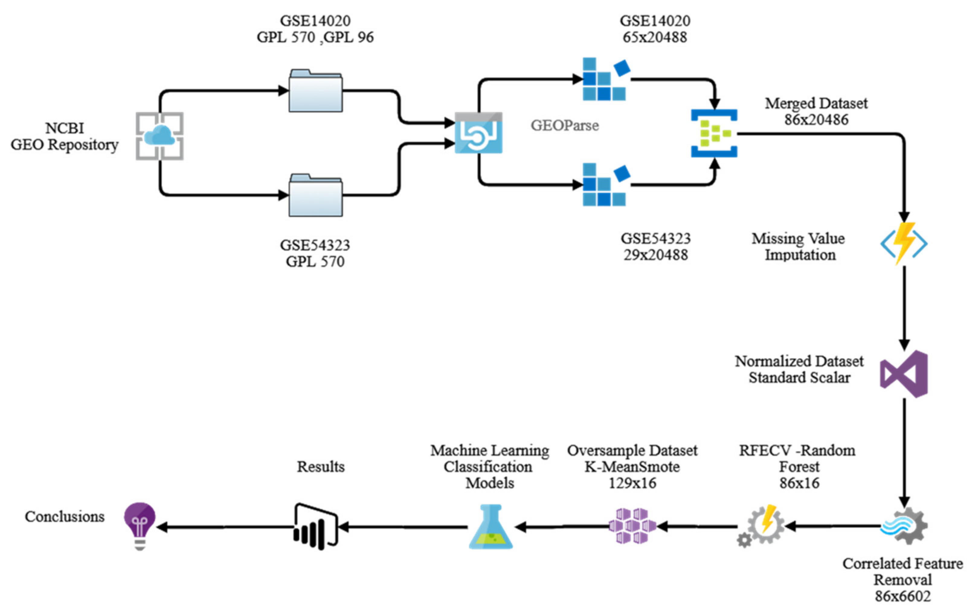
The lungs are the second most common location for metastatic development with 20–54% pulmonary secondary tumor. BC, colorectal, and renal cancer are the most common predominant laceration leading to BCLuM in adults. In some instances, the cause remains unclear and could be listed as the unknown primary cancer. Pulmonary metastatic disease may have heterogeneous clinical features and may have signs or symptoms with or without them. The BCLuMs are most often associated with endovascular distribution in the distal arterial pulmonary circulation of tumor cells [22]. The lungs would be the first sizeable capillary bed a BC cell faces after it has escaped into the bloodstream. As a CTC in the lungs, they can contact blood vessels of up to 100   m 2 . Since these CTCs are five times bigger than the tiny pulmonary capillaries in these capillary beds, the risk of BC cell detention and eventual extravasation into the lungs is high [1]. In reality, about 60% of metastatic BC patients eventually suffer metastases of the bones or lungs in their lives. BC patients are highly vulnerable to BCLuM. Life expectancy is poor with median survival just 22 months after BCLuM treatment. In particular, BCLuM was diagnosed for 60–70% of metastatic BC patients who finally died [23].

2.6. Methodology

In this work, datasets were transformed into a readable format. The selected dataset contains gene expression microarrays of different dimensions that need to be merged based on a common platform (GPL570) and a unique gene identifier (Entrez ID). Data were imputed for missing values and normalized. Gene expression data is known to have the curse of high dimensions. First, highly correlated features were removed and then two-dimensionality reduction techniques were employed to reduce dimensions to cater to this issue. Various classification models were employed with different tests and training split ratios to determine the best accuracy model. In the process, a handful of unique genes that can identify the metastasis location, i.e., brain, bones, lungs, and liver, were able to be identified in a BC patient. The authors of this research have not come across any study that has achieved the said objective. Figure 1 shows the proposed architecture for the identification of breast cancer in vital organs using microarrays.

2.7. Dataset (Dataset Availability)

Two datasets, NCBI-PubMed Gene Expression Omnibus (GEO) GSE14020 [11] and GSE54323 [12], are used in this research. The Gene Expressions Omnibus (GEO) project was launched to increase demands for a public repository of high-performance gene expression data. GEO provides a scalable and open architecture that allows the submission, processing, and testing of heterogeneous data sets from high-performance gene expression and genome hybridization studies. GEO does not plan to substitute internal gene expression databases, which gain from systematic data sets and are structured to simplify a specific analytical approach to function as a tertiary central data delivery center. GEO has three main data entities: samples; platforms; and series. These entities are designed for gene expression and studies on genomic hybridization.
In essence, a platform is a collection of samples that determine what molecules can be identified. A sample defines the collection of examined molecules and refers to a single molecular abundance data platform. A series organizes samples into coherent data sets. The GEO repository is publicly available in [24]. Dataset GSE14020 contains 65 samples collected using two platforms, GPL96 (36 samples with 22,283 gene probe ID) and GPL570 (29 samples with 54,675 gene probe ID) (Appendix A) whereas in dataset GSE54323 29 samples were collected using GPL570 (54675 gene probe ID) (Appendix B) summary in Table 1.
GPL96 is [HG-U133A] an Affymetrix Human Genome U133A array. Human Genome U133 (HG-U133) arrays allow the examination of gene expression across the genome or concentrating on a subset of well-defined genes using single or multi-array plate cartridges. HGU133 is based on the same gene information and identical sample technique to measure the gene expression thoroughly and reliably. GPL570 is [HG-U133_Plus_2] an Affymetrix Human Genome U133 plus 2.0 array. A systematic study of genome-wide expression in a single array, U133 plus 2.0 Array, analyses the relative expression above 47,000 transcript versions with over 38,500 well-known uni-genes and genes. It offers 9900 more samples, representing 6500 more new genes than the previous HG-U133 set with over 54,000 samples and 1,300,000 special features of oligonucleotides [25].
  • Entrez Gene
Entrez Gene is a gene-specific database (NCBI National Center for Biotechnology Information) located on the US National Institutes of Health Campus in Bethesda, MD, USA. Entrez Gene produces unique Gene ID (integers) as stable identifiers for a subset of model organisms for genes. It detects and uses such identifiers to incorporate various information including summary descriptions, nomenclature, gene-specific and gene product-specific sequence accessions, pathway and protein interaction reports, chromosomal localization, and related markers phenotypes. Since Gene ID is used in other NCBI databases to describe gene-specific information, the complete Entrez Gene report contains a wealth of links to citations, sequences, variants, homologs, and databases of gene-specific literature beyond NCBI [26].

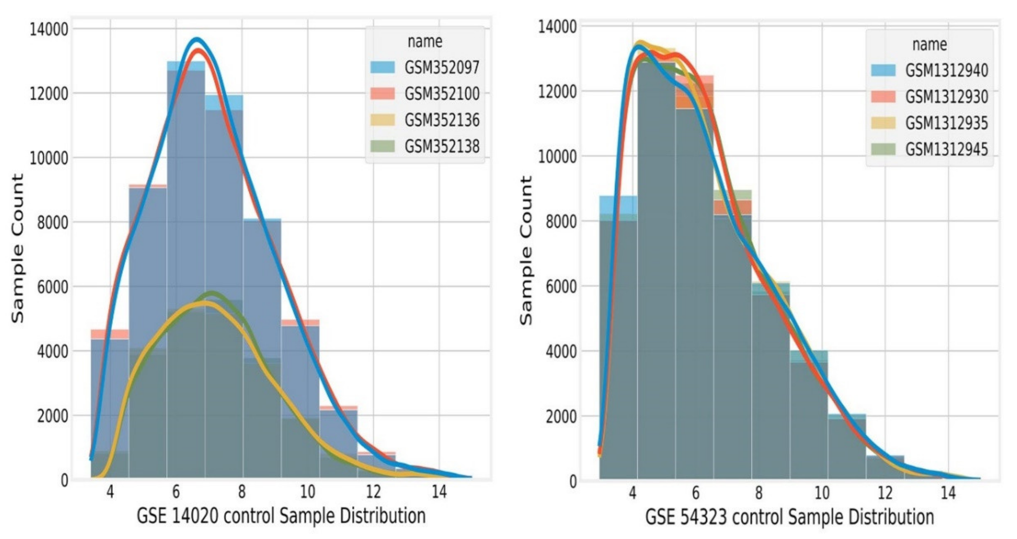
2.8. Data Pre-Processing

Merging of datasets is inevitable, but the raw data (SOFT files, i.e., simple omnibus format in text) must go through pre-processing before that. The GEOParse package was used in this study to facilitate the researchers in genome studies and download and load the SOFT files from the Gene Expression Omnibus database.
  • SOFT Files
The Simple Omnibus Text Format (SOFT) is designed to submit and download data quickly. SOFT is a simple line-based, plain text format that allows SOFT files from regular spreadsheet and database applications. A single SOFT file may contain data tables and descriptive information for samples, series records, and multiple platforms [27].
  • GEOParse
GEOParse is a python package used to query and retrieve data from the Gene Expression Omnibus database (GEO) [28]. Salient features of this library are:
Download GEO series datasets as SOFT files.
  • Download supplementary files for the GEO series to use locally.
  • Load GEO SOFT as easy to use and manipulate objects.
  • Prepare data for GEO upload.
In this study, datasets are GSE14020 and GSE54323. All the respective samples from each dataset are downloaded in a data frame (data arranged in tabular format as rows and columns).

2.9. Data Transformation

Dataset GSE14020 contains 65 samples collected using two platforms, GPL96 (36 samples with 22,283 gene probe ID) and GPL570 (29 samples with 54,675 gene probe ID), whereas dataset GSE54323 29 samples were collected using GPL570 (54,675 gene probe ID). Samples are collected using different platforms with different numbers of gene probe IDs. To induce uniformity across the dataset, samples were merged based on the common platform GPL570 (22,283 gene probe ids) and Entrez Gene ID (Unique Gene record identifier), thus reducing the number of features/gene probes IDs to 20,486. The dataset shape achieved after transformation is 86 × 20,486 and X = { x 1 , x 2 , x 3 , x 4 , x n } where x 1 , x 2 , x 3 , x 4 , x n are the features/independent variables and y prognosis location of metastasis ( lungs ,   brain ,   bones ,   liver ) . The distribution of four controlled samples is shown below in Figure 2. The histogram’s careful analysis shows that samples are not normally distributed; instead, it is right-skewed. The data, therefore, needs transforming for further processing.
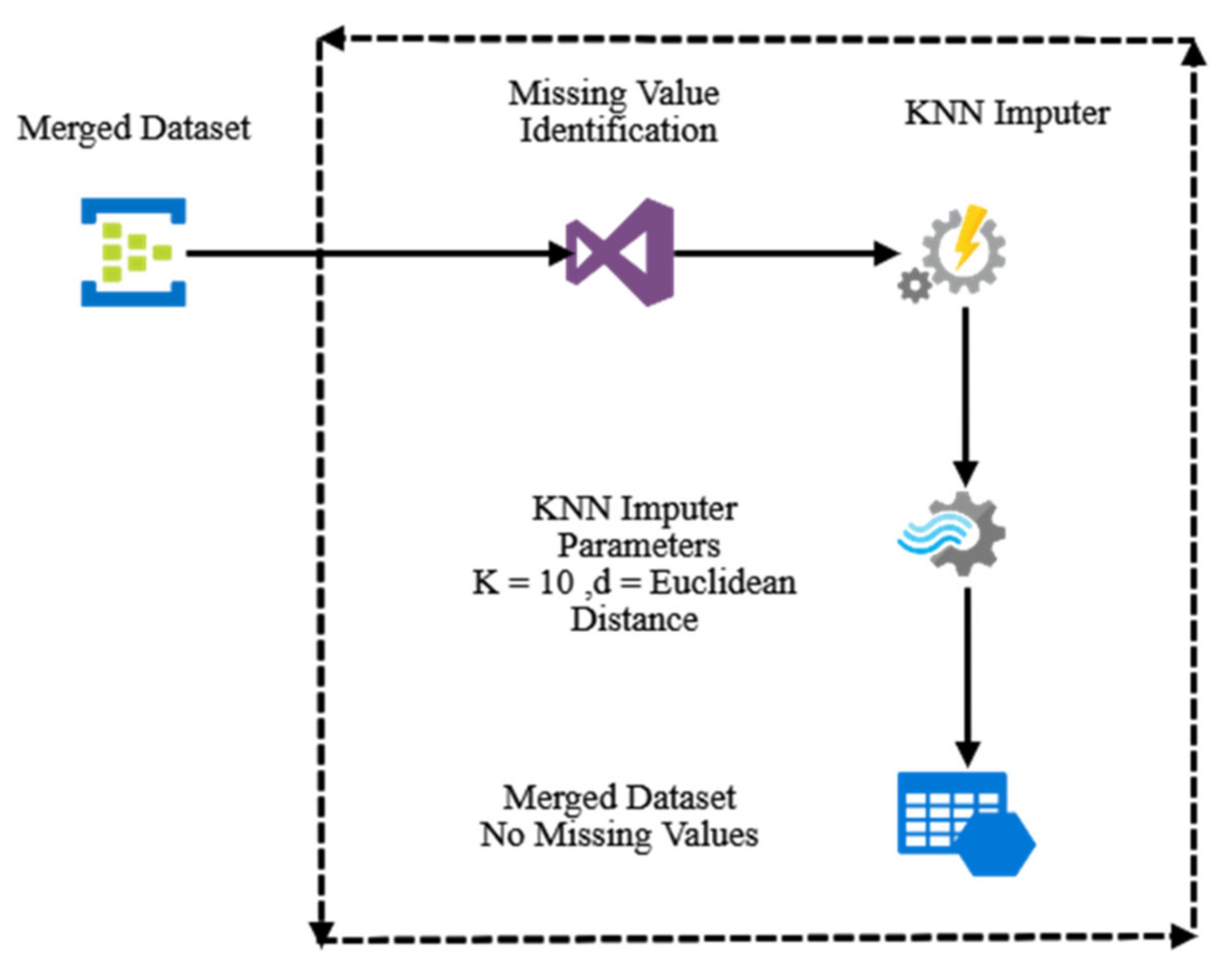
  • Missing value imputation
The gene expression details from microarray experiments are usually in large matrices of rows (gene expression level) and columns (various experimental environments). Although microarray technology is widely used, the information obtained mostly suffers from missing values. Microarray data may include missing values of up to 10%, and (in some cases) 90% of genes have one or more missing value in some data sets. Missing values exist for numerous reasons including microarray artifacts, inadequate resolution, hybridization, image noise, and corruption.
Furthermore, suspicious values are also sometimes reported as missing values. The presence of missing values in gene expression may harm subsequent research. Missing values are found to give specific algorithms a non-trivial negative effect. Repetition of experiments can be avoided by imputing missing values. Different algorithms are available for imputing the missing values in gene expression [29].
The imputation process for missing values exploits two data types from the data matrix. The first type is an existing correlation in the data matrix. Since the gene is involved in similar cellular functions, the gene expression data matrix has an identical gene expression profile. A correlation exists in rows and columns under the same genes—similar behavior under similar conditions. The second type is domain expertise of data or the process itself. The experience in the domain is highly beneficial to estimate missing values. Algorithms used for missing value imputation can be categorized as global and local approaches. The global correlation information is extracted based on the entire data matrix, whereas in a local approach only a subset of genes is used to show a gene with a missing value and high correlation value. K-nearest neighbor imputation (KNN impute), the earliest and most well-known imputation algorithm, has been used in this study. KNN impute falls under the category of local approach. Missing values in the dataset are shown in Appendix A, highlighted in red.
  • KNN (K-nearest neighbors) impute
This differs from other approaches as it does not work with an actual mathematical model. On the contrary, the inference is performed by comparing new samples with existing ones (defined as instances). KNN is an approach that can be easily employed to solve clustering, classification, missing value imputation, and regression problems. The main idea behind the clustering algorithm is straightforward. Consider a data generating process p data and a finite dataset is drawn from this distribution:
X = { x 1 ¯ , x 2 ¯ , x 3 ¯ , x 4 ¯ x n ¯ }
where x i ¯ R N
d p   =     x 1 ¯ ,   x 2 ¯ =   Σ j = 1 N   x 1 j     x 2 j   p   1 / p
where p = 2 , d p represents the classical Euclidean distance, which is usually the default choice. In particular cases, it can be helpful to employ other variants such as p = 1 (the Manhattan distance) or p > 2 . Even if all the properties of a metric function remain unchanged, different values of p yield results can be semantically diverse. The KNN algorithm determines the K closest samples of each training point. When a new sample is presented, the procedure is repeated with two possible variants:
  • With a predefined value of K, the KNN is computed.
  • With a predefined radius/threshold r, all the neighbors whose distance is less than or equal to the radius are computed.
The philosophy of KNN is that similar samples can share their features. For example, a recommendation system can cluster users using this algorithm and, given a new user, find the most similar ones (based, for example, on the products they bought) to recommend the same category of items. In general, a similarity function is defined as reciprocal of distance (there are some exceptions, such as the cosine similarity):
s = x 1 ¯ , x 2 ¯ = f d p x 1 ¯ , x 2 ¯ = 1 d p x 1 ¯ , x 2 ¯ for   d p x 1 ¯ , x 2 ¯ 0
Two different users (A and B), who are classified as neighbors, will differ under some viewpoints, but at the same time, they will share some peculiar features. This statement authorizes one to increase the homogeneity by suggesting the differences. For example, if A liked the book b1 and B liked b2, we can recommend b1 to B and b2 to A. If this hypothesis were correct, the similarity between A would be increased; otherwise, the two users will move towards other clusters that better represent their behavior [30]. The missing data is used as the test case for the imputation of the missing value. Available and missing features represent input feature space and class label (output). Its K-nearest neighbors from exclusive features are identified whose label imputes the missing attribute [31].
  • The KNN-based method
The KNN approach chooses gene expressions identical to the gene, in which missing values can be imputed. In experiment 1, assume gene A has one missing value. This method will classify K additional genes with a value obtained in experiment 1, with an expression identical to A in experiments 2-N (N is total experiments). The missing value in gene A is estimated from the weighted average values of K closest genes. Each gene’s contribution is weighted on a weighted average by the gene expression similarity to gene A. After evaluating several matrices for gene similarities such as the Euclidean distance, Pearson correlation, and variance minimization, the Euclidean distance was reasonably accurate. It is pretty surprising provided that the Euclidean distance is sensitive primarily to outliers. Outliers are most likely to exist in microarray data, however, log base2-transformation significantly reduces the outlier’s effect on gene similarity [32].
As shown in Figure 3, in this study, K-nearest neighbors are used to input missing values. Each sample’s missing values are changed using K = 10 .
( K = 5 10 is a good choice for gene expression arrays missing value imputation in human tumors) [33]. Adjacent neighbors’ mean values, the closest neighbor in the training set, and weights by inverse distance. The distance here is the Euclidean distance. More immediate neighbors to a point under query would have a more significant effect than the farthest neighbors in this scenario. The two samples are close if the features that neither is missing are close [34].
  • Data Normalization
Generally, the feature values range varies widely in various databases. When feature values vary, several training algorithms’ objective function does not operate correctly. Assume that the algorithm’s objective function uses the distance between two features; the feature controls the distance with an extensive range of values that deceive the objective function. Similarly, the gradient-based back-propagation algorithm performs better if the attribute values are of the same range. The features are scaled to a specified range to eliminate one factor’s influence over another and faster convergence. Data normalization is the process by which feature values are scaled to a specified range. In microarray data, the value of the attributes ranges from a low to an enormous value. This paper has already shown the sample distribution in Figure 2, which indicates that the data needs to be normalized. Therefore, data normalization is unavoidable for the microarray dataset before applying any training algorithm. Here, the standard scaler normalization method is applied to scale the data [35]. Independent variables or features are standardized to zero mean and scaling to unit variance. The standard score is calculated as:
Z i = x i μ σ
  • Where mean: μ = 1 N Σ i = 1 N x i and standard deviation:
    σ = 1 N Σ i = 1 N x i μ 2
The normalized dataset after merging is shown in Appendix C.
  • Removal of Correlated Variable
A multivariable analysis is a widely used statistical tool in medical research if the correlation of several predictive variables with study measurements is calculated. However, the multivariable efficiency of analysis depends on the correlation structure between predictive variables. Moreover, the multivariable efficiency of analysis also depends on the correlation structure between predictive variables. The multivariate analysis assumes that all predictive variables are not correlated. Multi-collinearity or issues arise when the model’s covariate is not independent. Consequently, it leads to biased coefficient estimation and loss of power in genomics and medicine studies. Statistically, correlation assesses a linear association among two continuous variables.
Correlation is measured by the correlation coefficient, representing the strength of linear association between the variables. A correlation coefficient of zero means that two continuous variables have no linear relationship and a correlation coefficient of −1 or +1 reveals an entirely linear relationship. The higher the correlation, the closer the correlation coefficient gets to ±1. The variables are positively related if the coefficient is a positive number and the variables are inversely related if the coefficient is a negative number. There are two key correlation coefficients, i.e., Pearson’s correlation and Spearman’s rank correlation coefficient. The proper application of the correlation coefficient form depends on the type of variables under study [36]. In the study, only Pearson’s Correlation coefficient is being considered. Pearson’s correlation coefficient is denoted as ϱ for a population parameter and as r for a sample statistic. Pearson’s correlation between variables x and y is given by:
r = Σ i = 1 n x i x y i y Σ i = 1 n x i x ¯ 2 Σ i = 1 n y i y ¯ 2
Before proceeding further, the highly correlated features were removed. All the independent variables having a Pearson correlation coefficient greater than 0.8 or less than −0.8 were removed. 13,884 features were removed, thus reducing the reduced dimension of the dataset to 86   ×   6602  Appendix D.
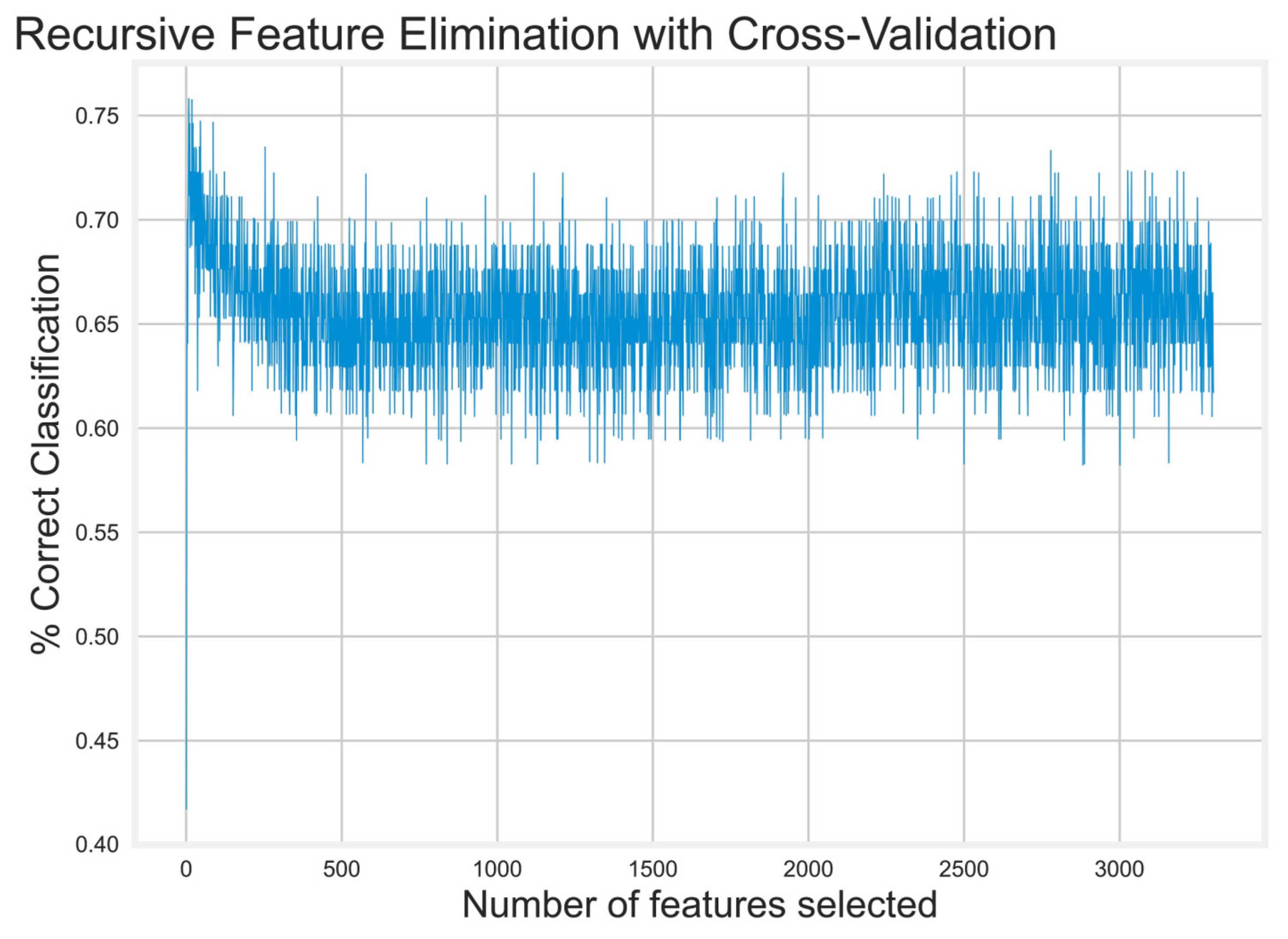
  • Dimensionality Reduction
Even after removing highly correlated features, the dimensions of the dataset were still too large to handle. Next, the recursive feature elimination technique was used to reduce the dataset’s dimension further. Moreover, RFE (Recursive Feature Elimination) will identify the most robust predictor/features.
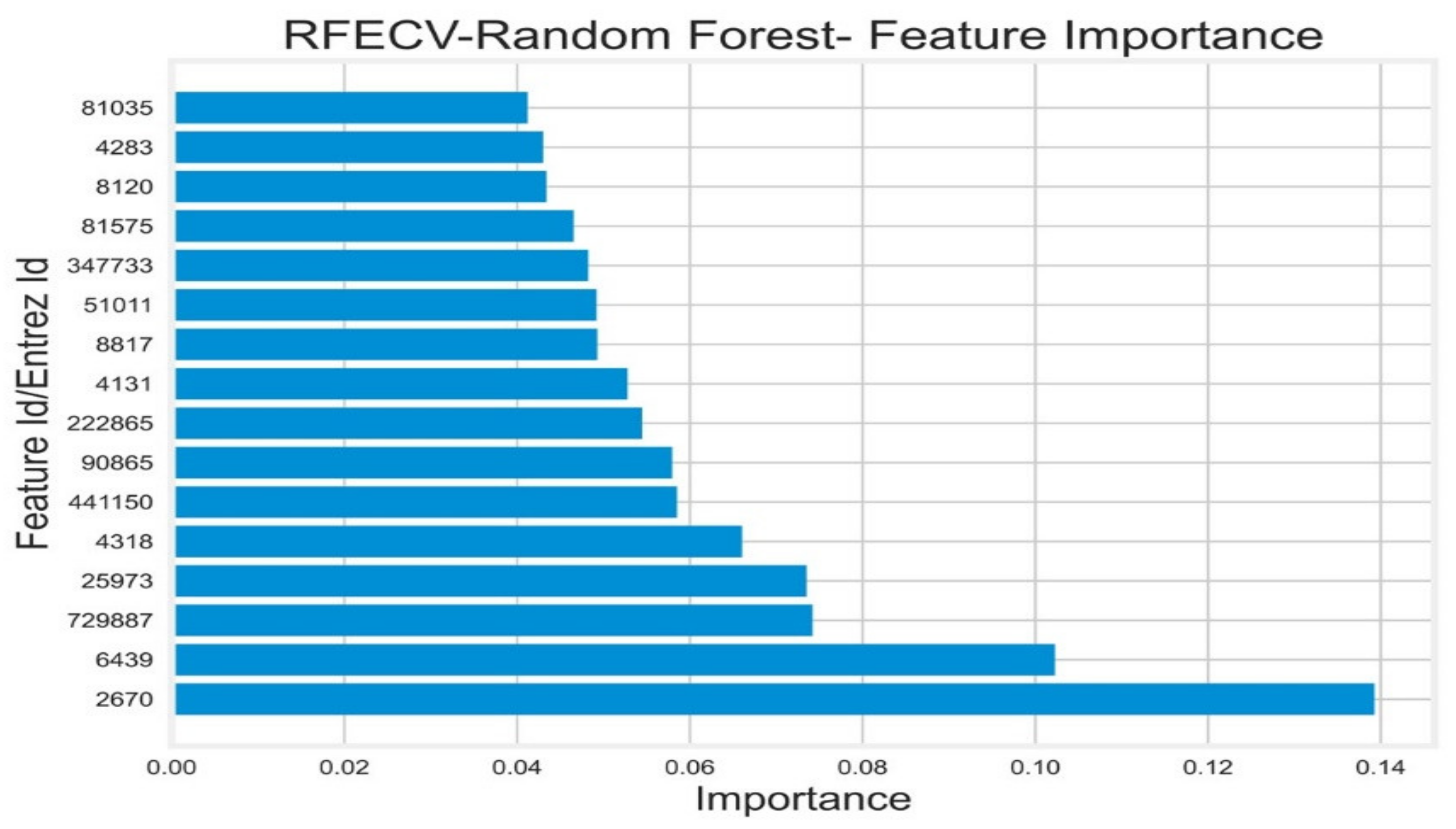
  • Recursive Feature Elimination (RFE)
Random forest (RF) is a supervised machine learning algorithm. It generally works well with high dimensional datasets and can recognize a given result’s strong predictors without making any basic model assumptions. However, correlated predictors are a common problem with high-dimensional data sets. RF’s efficiency in recognizing the most potent predictors decreases the significant calculated scores of correlated variables. Highly correlated variables were already removed in the last step. The Random-Forest-Recursive Feature Elimination (RF-RFE) algorithm is a proposed solution. RFE performs the selection of features by iteratively training a model, classifying features, and eliminating the lowest ranking attributes [37]. RFE needs a range of features to be preserved. However, the number of features that are authentic is also not decided in advance. Cross-validation is used with RFE to score specific feature subsets and select the best scoring collection of possible features or attributes. In this experimental study, the Stratified K-fold cross-validation was used for recursive feature elimination. Stratified K-Fold shuffles the data split into n_splits parts. Each split is used as a test set. It constantly shuffles data once before splitting and does not overlap test sets.
Recursive Feature Elimination with Random forest with stratified K-fold cross-validation reduced the optimal number of features from 6602 to 16. The optimal number of features and their importance is shown in Figure 4 and Figure 5 below.
  • Class imbalance
The critical problem in microarray data analysis is a limited sample size with high dimensionality. Class imbalances compound this situation. Data imbalance concerning multiclass classification has been recognized as a challenging problem for machine learning techniques as it directly impacts the classification model’s performance. Most of the machine learning classification algorithms assume the classes to be balanced. As a result, the algorithm would favor the majority class and ignore the minority classes leading to poor classification models, leading instantiation, and poor performance metrics. The class imbalance will reduce the credibility of the accuracy of classification. In addition, notable features with an imbalanced data set are often problematic as they are not evenly distributed in the training set [38].
In the following datasets is the status of class imbalance in two datasets, GSE14020 and GSE54323. Figure 6 and Figure 7 show the imbalanced nature of the two datasets.
After the merging of two datasets, The overall class imbalance situation of a dataset is shown in Figure 8.
The number of observations for site (sub-cutaneous site) and node (Lymph Node) were not significant. These samples were dropped before proceeding further, as shown in Figure 7.
  • SMOTE
Over time, various resampling techniques have emerged to cater to the class imbalance problem. Frequently used methods are over-sampling and under-sampling. The underlying principle of these methods is to randomly remove samples or randomly pick samples from the minority and replicate them, causing either information loss or overfitting. SMOTE is a prevalent resampling technique used in imbalance classification datasets. SMOTE (synthetic minority oversampling technique) is an approach that oversamples the minority class by creating synthetic examples rather than creating over-sampling with replacement. Synthetic samples are explicitly generated by acting in the feature space instead of the data space. The minority classes are oversampled by selecting each minority class sample and inducing synthetic samples along the line, joining any minority class nearest neighbors. Nearest neighbors are randomly chosen based on the aggregate of over-sampling required. For example, suppose the aggregate of over-sampling needed is 300%. In that case, only three neighbors are selected (based on five nearest neighbors) and only one sample is created synthetically in each direction. New synthesized samples are created as the difference between the feature vectors, i.e., the sample being considered, and the nearest neighbor associated with it. This difference is multiplied by an arbitrary value between zero and one and then added to the feature vector considered. Consequently, it causes the arbitrary point to be selected along the line segment between two specific features. Therefore, this method dictates the decision region of the minority class towards more generalization [39].
The SMOTE samples are two similar linearly combined samples of minority class x   and   x R and are defined as:
S = x + μ · x R x
0 μ 1 ;   x R is randomly chosen among the five-minority class nearest neighbors of x . In this study, K-means SMOTE [40] has been used. K-means SMOTE assists classification by generating minority class samples in safe and crucial areas of the input space. The technique prevents noise generation and overcomes imbalances between and within classes effectively. K-means SMOTE works in the following steps:
  • Use the K-means cluster algorithm to cluster entire data.
  • Choose clusters with a significant number of minority class samples.
  • Assign more synthetic samples to clusters with sparse distribution of minority class samples.
Figure 9 depicts the balanced data samples in each class after applying the K-means SMOTE oversampling technique.
Since the data from 86 × 16 to 129 × 16 has been oversampled, the dataset’s final shape is shown in Appendix F [41].
  • Sampling
In this study, the Stratified shuffle split was sued for sampling. Stratified sampling tends to split a data set so that each split is identical to something. A classification setting is always chosen to ensure that training and test sets have roughly the same samples for each target class as the complete set. A 70/30 ratio was employed, i.e., splitting the dataset such that 70% of the samples are reserved for training the model and 30% of the samples for model validation. The dimension of the training dataset was 90   ×   16 and the test dataset was 39   ×   16 .

2.10. Classification Models

Four different models have been trained based on different classification techniques used for multiclass classification. A brief description of these algorithms is shown below.
  • K-nearest neighbor (KNN)
KNN is used for both regression and classification problems. It belongs to the family of supervised learning algorithms. It uses feature similarity to predict the class y for a new set of observations x. It has extensive pattern recognition and classification application and uses information about the neighboring points to classify output labels. KNN classifier is an example-based learning and non-parametric algorithm. It performs well even if the data is non-Gaussian. This algorithm does not learn the model, instead, it learns the training instances that are the foundation of information during the prediction phase. This algorithm uses k distance estimates based on input features. The optimal value of k = 3 is used in this research. However, non-relevant features significantly reduce the accuracy or precision of KNN, even with highly efficient classification. KNN has the downside of not being computationally efficient since it stores the whole training data in memory. Prediction of every new set of observations is required to run down through the full dataset, making it a lazy learning algorithm [42,43].
  • Decision Trees (DTs)
DTs are supervised learning and non-parametric methods used extensively for regression and classification. DTs predict the target variable y by learning straightforward decision rules inferred from input features x. A DT is a piecewise constant approximation that breaks down the training dataset into smaller sets with simple if-then-else decision rules. The outcome is a tree with decision nodes. DT classifiers build decision trees for a set of training data. The classifier frequently visits all decision nodes and chooses active splits until a leaf is pure and no further splits are obtainable. Several methods are available to quantify the purity of decision nodes, but the Gini impurity criterion has been employed in this research. DTs can create complex trees that do not generalize well, resulting in an over-fitted model. This problem can be avoided using the maximum depth of the tree. In this research max _ depth = 3 [44] has been used.
  • Random Forests (RF)
RF is a supervised and non-parametric learning algorithm. RF is suitable for both regression and classification. However, its main application is in classification. RF is an ensemble learning method that is superior to a DT as it mitigates the over-fitting and minimizes the influence of outliers on predictions. Random forests are merely a collection of DTs. In RF, each tree is different from one another. A single tree might be good at predicting, but most likely be overfitting on another part of data. The overfitting can be reduced by averaging the results of multiple decision trees, while retaining the predictive power. Random forest employs the same strategy by inducing randomness to ensure that each tree is different and distinct. In order to build a tree, a bootstrap sample of data is taken. This process is repeated, thus creating a dataset as extensive as the original training dataset. However, RF selects a subset of random features and looks for the best possible test involving those features. These subsets of features are repeated on each node so that each node in a tree can be decided using a different subset of features. In this study, the maximum depth of the tree, max _ depth = 2 , has been used and the criterion to determine the purity of the node is Gini. In regression tasks, results are the average for prediction. A voting mechanism is used in classification making a soft prediction with the probability for each possible output label. The probabilities predicted by all the trees are averaged, predicting the label with the highest predicted probability [45,46].
  • Support Vector Machine (SVM)
SVM is the most popular and extensively used machine learning algorithm for classification problems. SVM predicts the target labels by creating a decision boundary between classes using single or multiple feature vectors. A decision boundary or hyperplane is a line that splits the input variable space by its class. The margin is the distance between the points that lie closest to the line. The hyperplane with maximal-margin is an optimum line that separates the classes with the most significant margin. The vertical (i.e., perpendicular) distance from these closest points to the hyperplane is the most relevant point in defining the classifier’s hyperplane and construction. These points are the support vectors that define the hyperplane. SVM was initially proposed to construct a linear classifier, however, a brilliant trick for SVM is a kernel function that enhances the capability to model non-linear higher dimension models. Kernel function adds dimension to input data and makes a non-linear problem to a linear problem in a higher dimension; it calculates the scalar product between two data points in a higher dimension space without explicit mapping from the input data to higher dimensions. There are three types of kernel functions used in SVM: polynomial; linear; and radial. This research study uses Grid Search CV (Grid Search Cross Validation) to find the optimal hyperparameter for its model. Kernel   =   Linear ,   C   =   1 ,   and   gamma   =   0.1 , where C is the L2 regularization parameter and gamma the kernel coefficient [47]. The above models were trained (70% data) and validated on the test (30% data) dataset.
A comprehensive summary of each classification model is presented in Table 2.

2.11. Classification Evaluation Metrics

In this study a multiclass classification problem is being dealt with. In classification problems, accuracy alone is not an excellent metric to validate a classifier. There are different performance metrics available for classifier evaluation. Classification model performance measures used in the study are:
Accuracy = TP + TN TP + TN + FP + FN
Precision = TP TP + FP
Recall / Sensitivity = TP TP + FN
Specificity = TN TN + FP
F 1   score = 2 × precision × recall precision + recall
True   Positive   Rate   ( TPR ) = Sensitivity
False   Positive   Rate   ( FPR ) = 1 Sensitivity
All the classifier models have been evaluated based on each classification model’s matrices and respective performance. Moreover, the models were compared based on ROC–AUC (receiver operator characteristic–curve area under the curve) and PR–AUC (precisionrecall—area under the curve) using Yellowbrick. AUC is the degree of separability, signifying the ability of the classifier to classify correctly.

3. Results and Discussion

Dataset GSE14020 contains 65 samples collected using two platforms, GPL96 (36 samples with 22,283 gene probe ID) and GPL570 (29 samples with 54,675 gene probe ID) whereas for dataset GSE54323 29 samples were collected using GPL570 (54,675 gene probe ID). Samples were collected using different platforms with different numbers of gene probe IDs. To induce uniformity across the dataset, samples were merged based on common platform GPL96 (22,283 gene probe IDs) and Entrez_Gene_ID (Unique Gene record identifier), thus reducing the number of features or genes probes IDs to 20,486. The dataset shape achieved after transformation was 86   ×   20,486 .
Furthermore, after removing highly correlated variables/features and reducing the dimensionality of the dataset to 86   ×   16 , the dataset was oversampled using K-means SMOTE to balance class distribution. The final dimensions of the dataset were 129 × 16 . Pearson correlation was calculated for each independent variable concerning each other as denoted in Figure 10. All the features with negative correlation values are marked red, whereas positive correlations are black.
A heatmap of positive and negative correlated features is shown in Figure 11 and Figure 12.
This clearly shows that most features exhibit positive correlation but a few are negatively correlated. Analysis of the correlation table in the figures above reveals that 18% of values are strongly correlated ± 0.5 ± 1.0 , 34% are moderately correlated ( ± 0.3 ± 0.49 ) and 48% are in weak correlation ± 0.29 .
Four different classifiers were trained on 70% train, 30% test ratio and evaluated each classifier concerning the accuracy, precision, recall, ROC–AUC, PR–AUC, and F1score. The experiments were evaluated on a virtual machine (VM) with an Intel Xeon CPU ES-2690V4 @2.60 GHz having 12 vCPU and 24 GB of RAM.

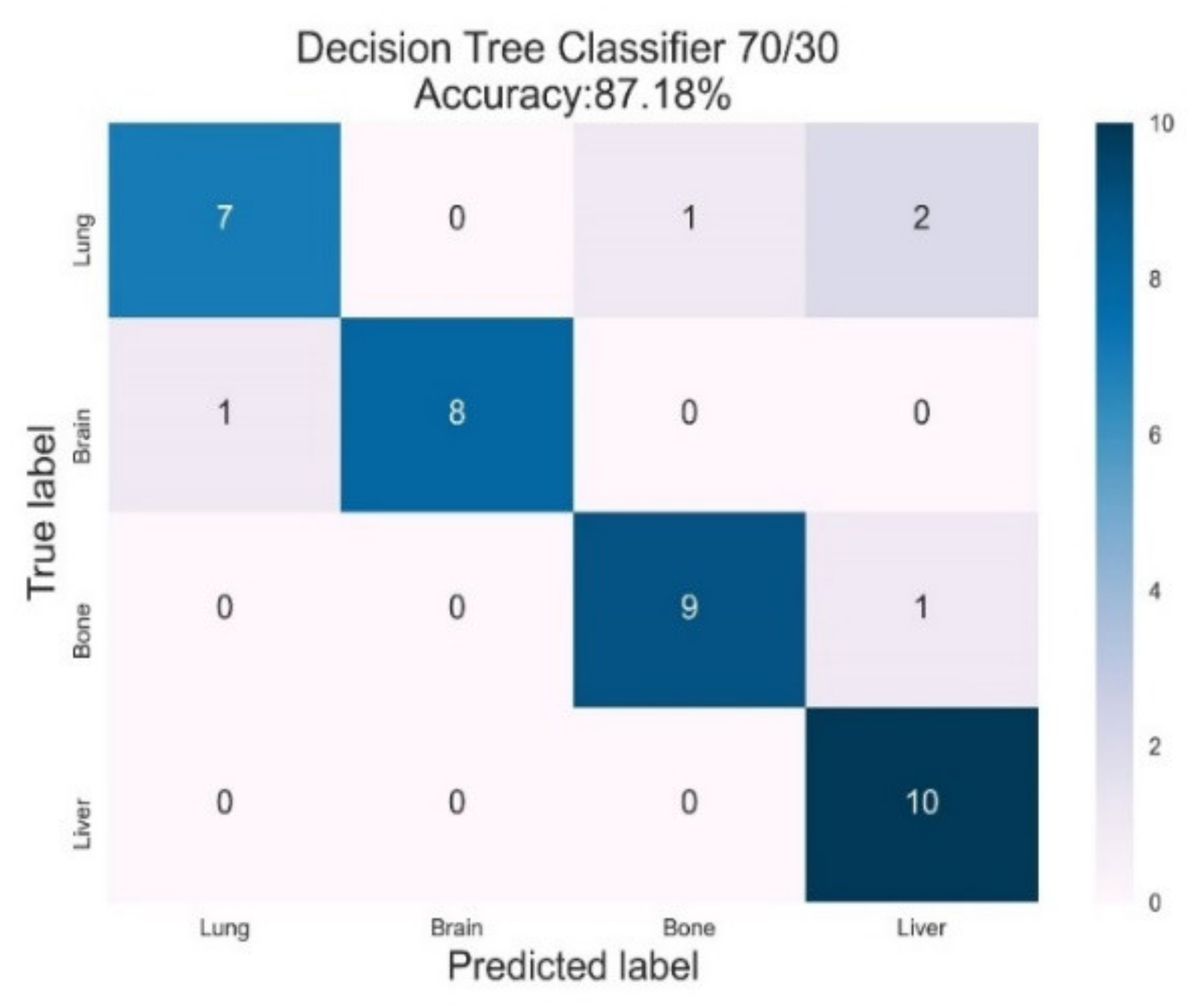
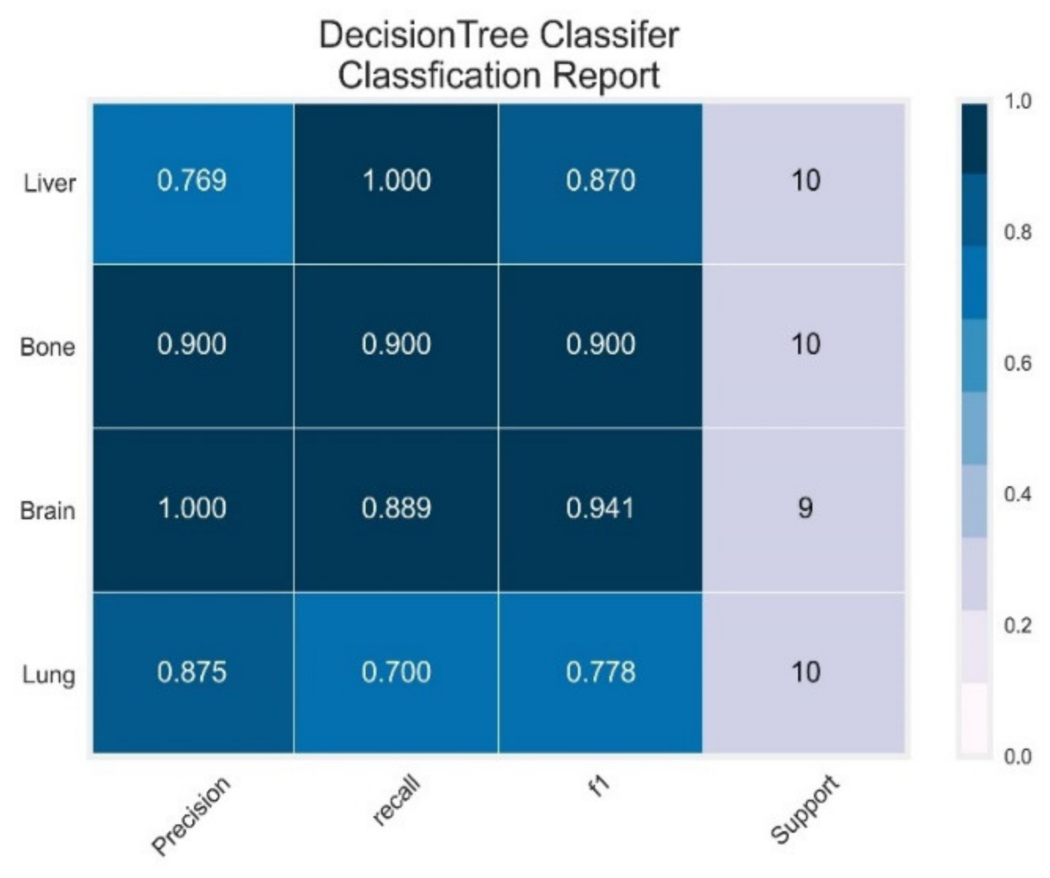
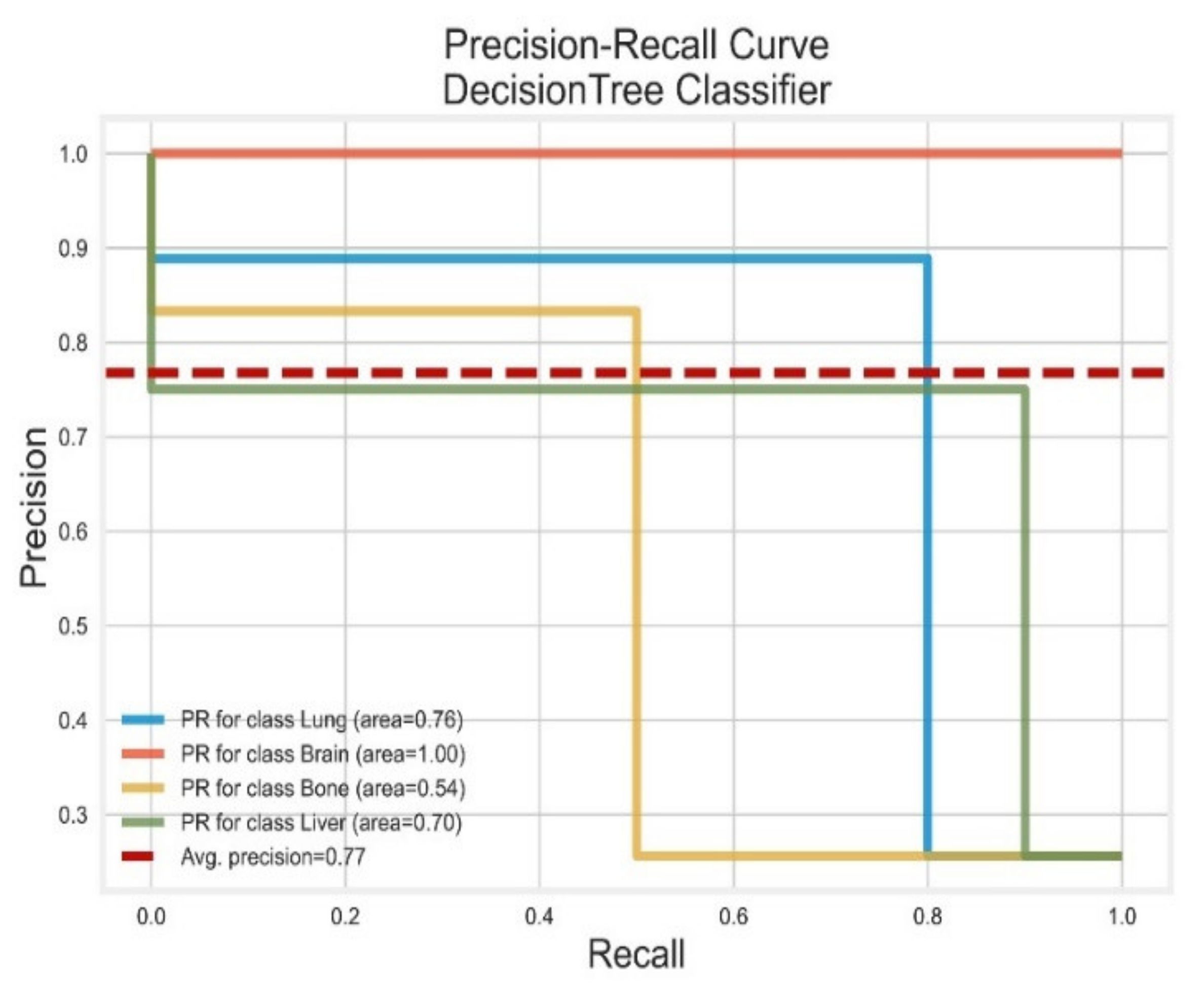
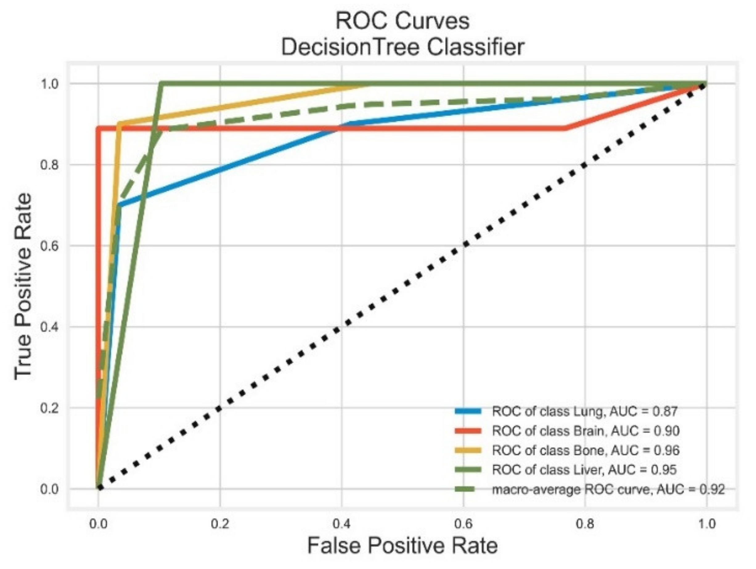
3.1. Decision Tree Classifier

Decision tree classifier had a training accuracy of 92% and validation/test accuracy of 87%. Confusion matrix is shown in Figure 13, which indicates the misclassified samples in lungs, brain, and bones class.
Out of 39 total samples, this classifier has misclassified five samples across all four classes. One lungs sample is classified as bone and two as liver, one brain sample is classified as lungs, and one bone sample as liver. The DT classification report is shown in Figure 14. Class liver and lung have low precision of 0.77 and 0.87, respectively, whereas lung has poor recall of 0.78, thus reducing the overall F1 Score for the liver and lungs class.
The precision-recall curve for DT classifier is depicted in Figure 15. Precision-recall curve is a metric to evaluate the quality of a classifier. It shows the trade-off between precision and recalls for each class. A larger area under the curve represents the classifier with high precision and recalls the best case scenario with an average precision of the classifier model.
The DT classifier had an average precision of 0.77, showing brain class with the highest PR AUC   =   1.0 , and bones with the lowest PR–AUC = 0.54. The Receiver Operator Characteristic (ROC) is shown for the DT classifier in Figure 16.
Higher TPR at low FPR indicates that it is a good model, whereas area under curve (AUC) is the separability of a classifier. The greater the AUC, the better the model is. AUC = 0.92 , indicating an excellent overall classifier.

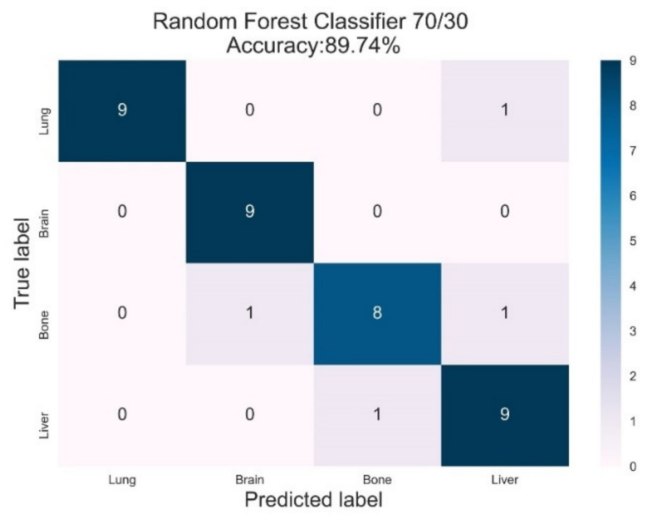
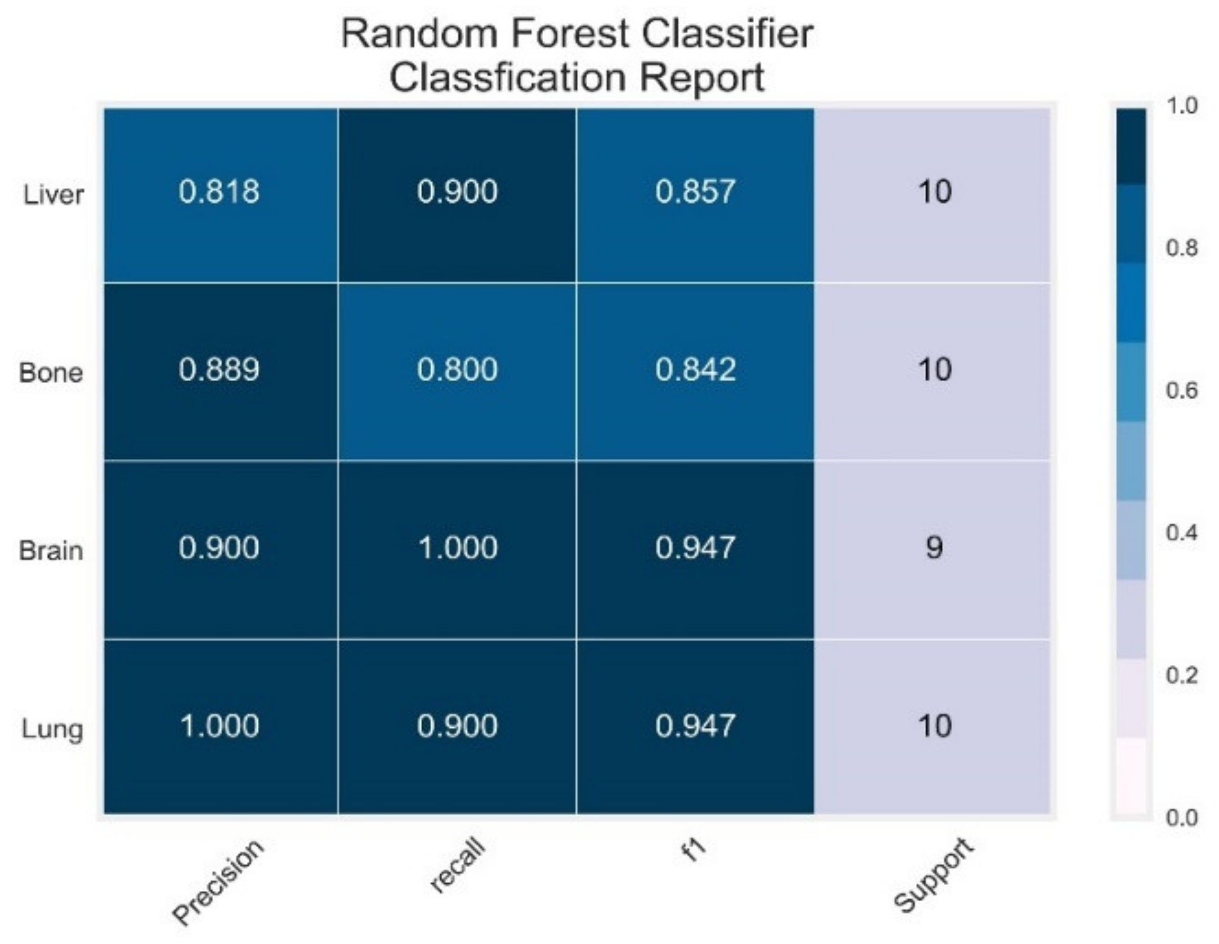
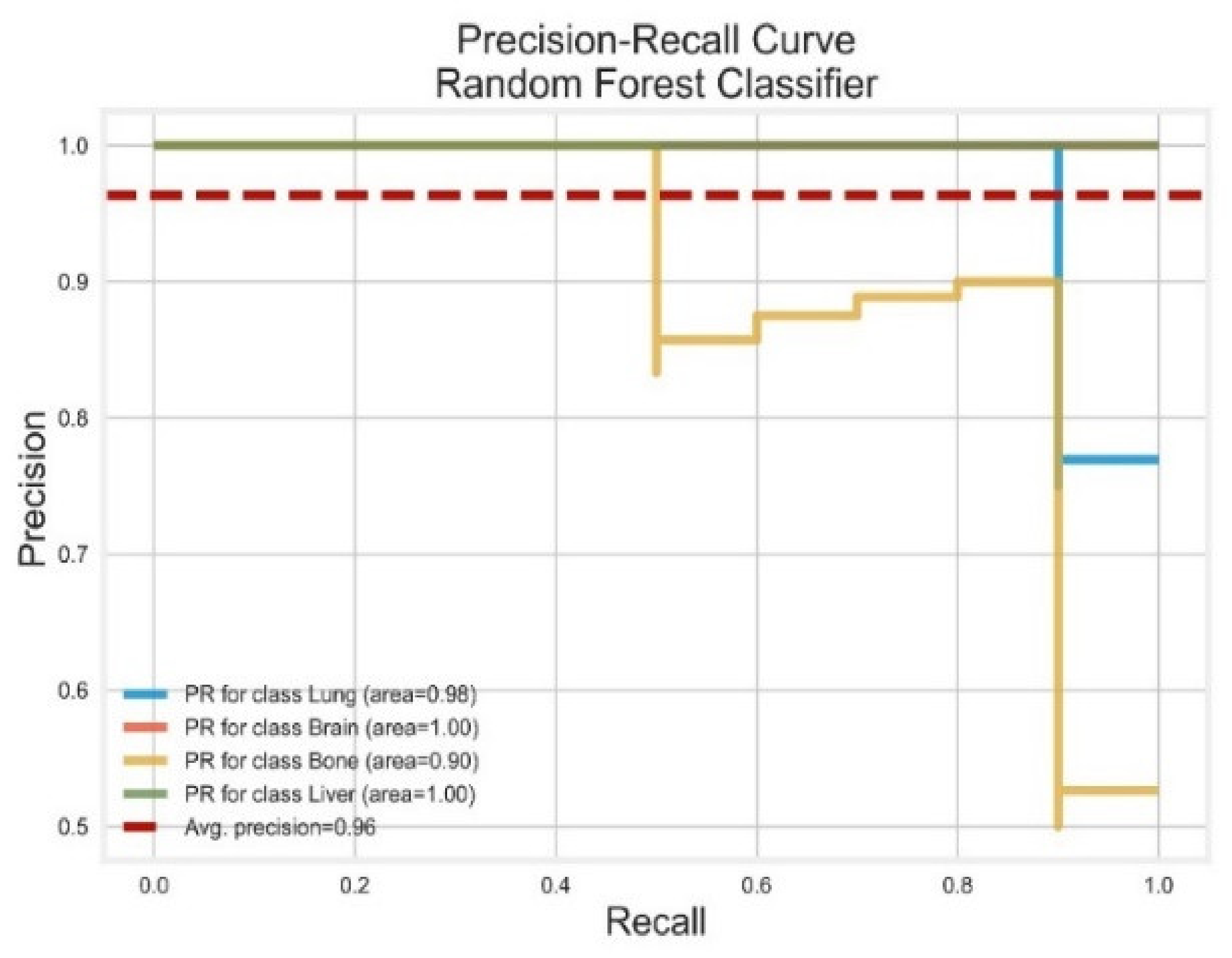
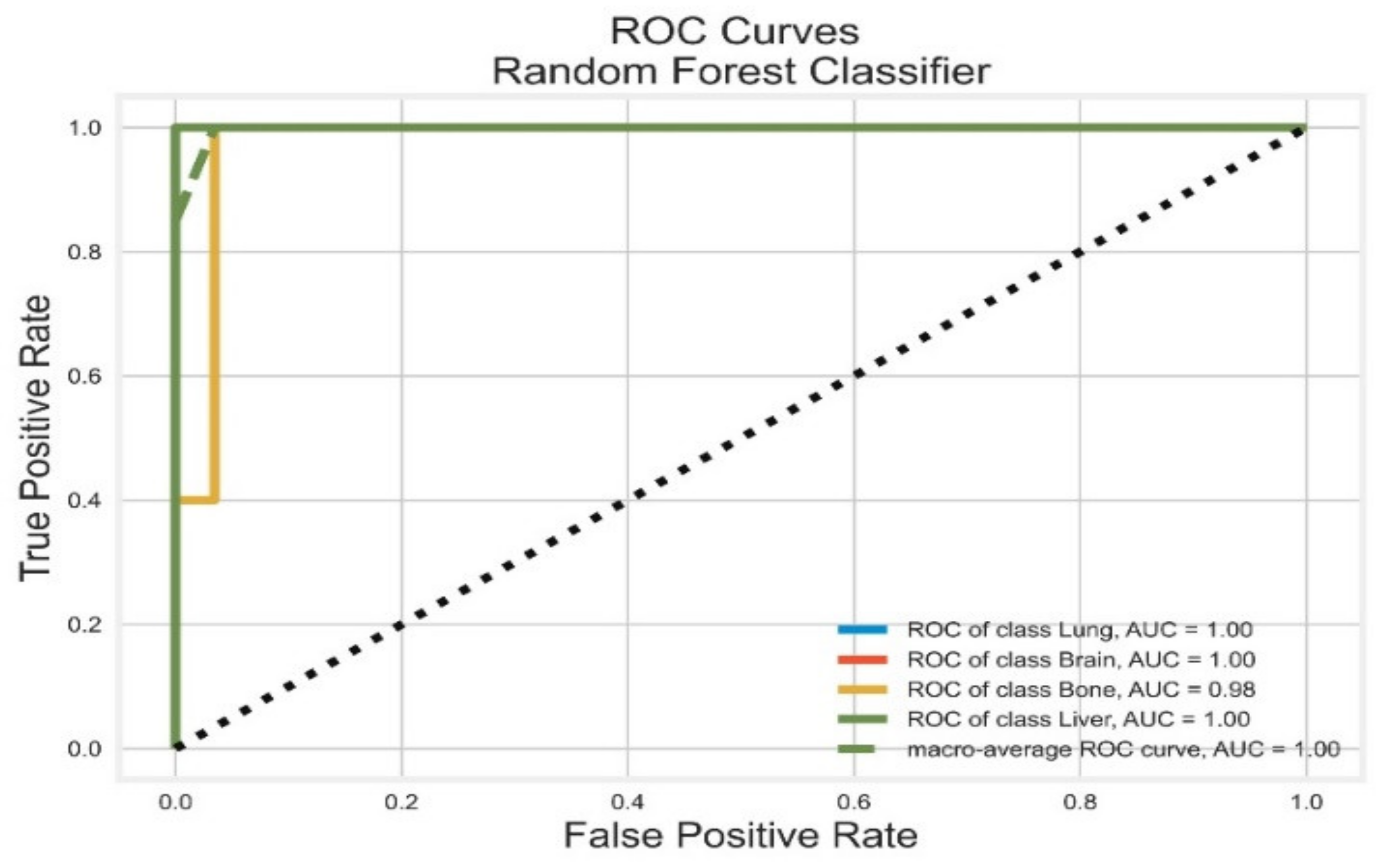
3.2. Random Forest Classifier

Random forest classifier had an overall training accuracy of 98% and validation /test accuracy of 90%. The confusion matrix of the classifier is shown in Figure 17. RF Classifier has misclassified only four samples out of a total of 39. One of the lung samples is classified as liver and two of the bone samples are classified as brain and liver, respectively. At the same time, one liver sample is classified as bone.
The classification report for RF classifier is shown in Figure 18. Class liver has a precision of 0.81 and bone with recall has a precision 0.80, thus reducing the overall F1 score for the liver and bone class to 0.85 and 0.84, respectively.
The precision-recall curve for the RF classifier is shown below in Figure 19.
The RF classifier had an average precision of 0.96, whereas all classes have PR AUC     0.90 , exhibiting a good classifier model. The Receiver Operator Characteristic (ROC) is shown for RF Classifier in Figure 20.
The average AUC = 1.0 for the RF classifier model where each class has an AUC     0.98 . The classifier is showing better separability among all classes and prediction power.

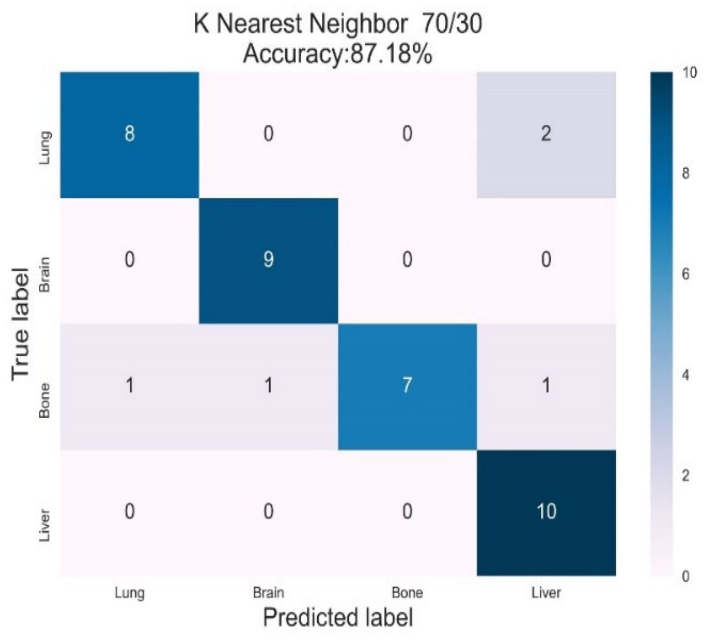
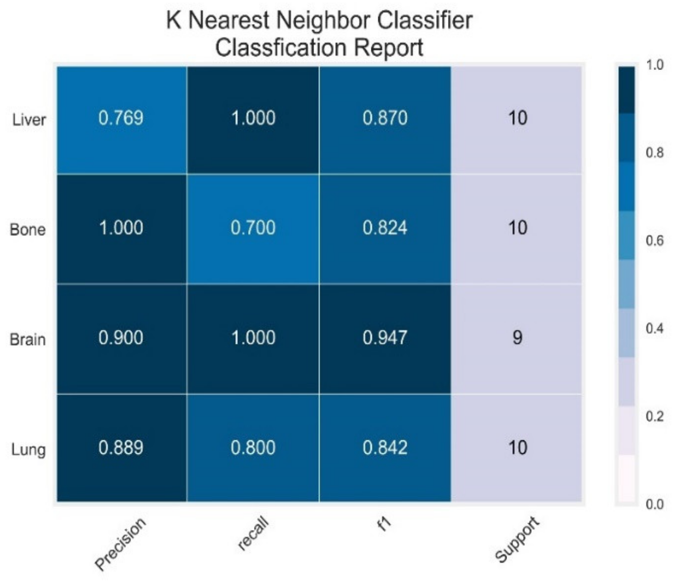
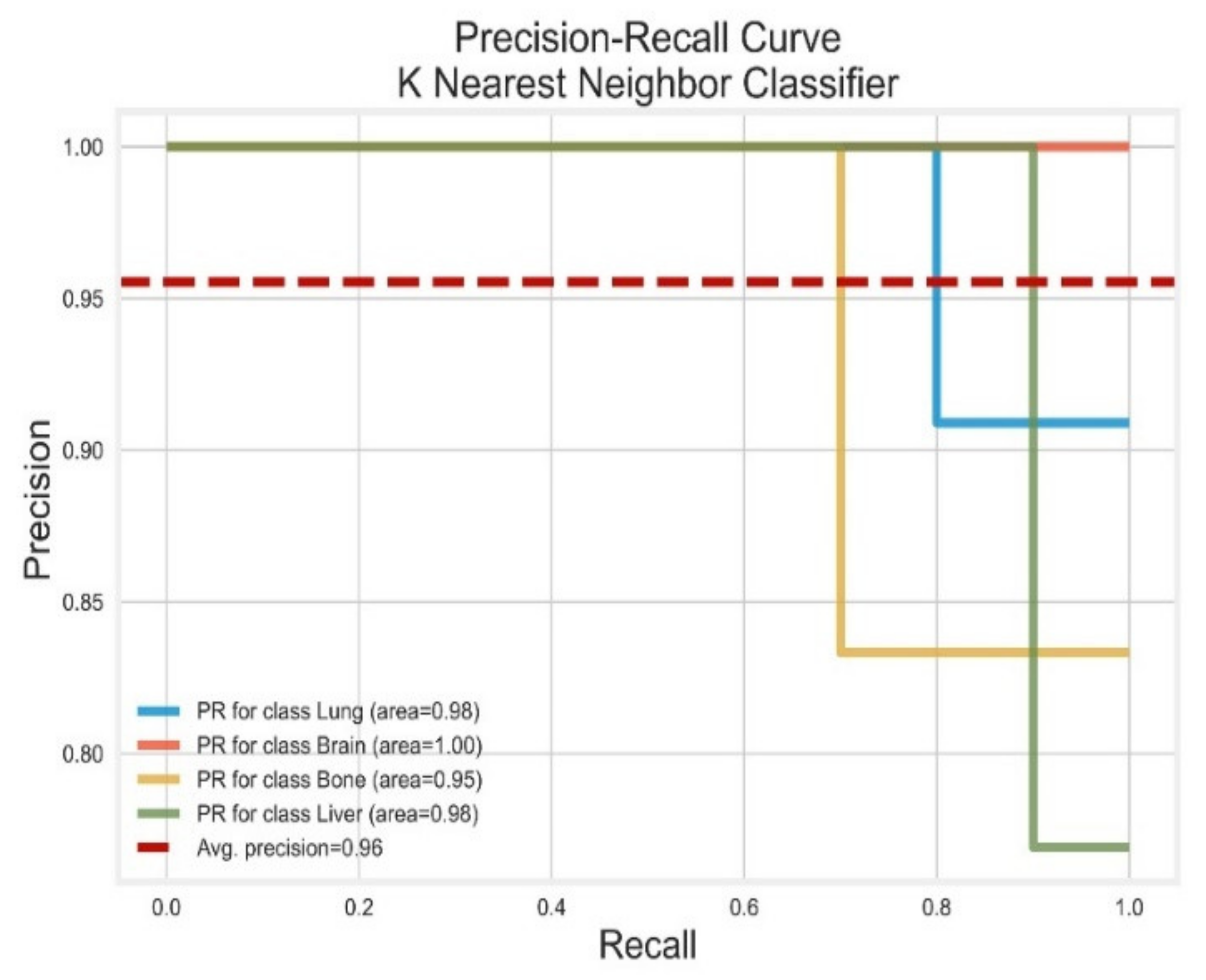
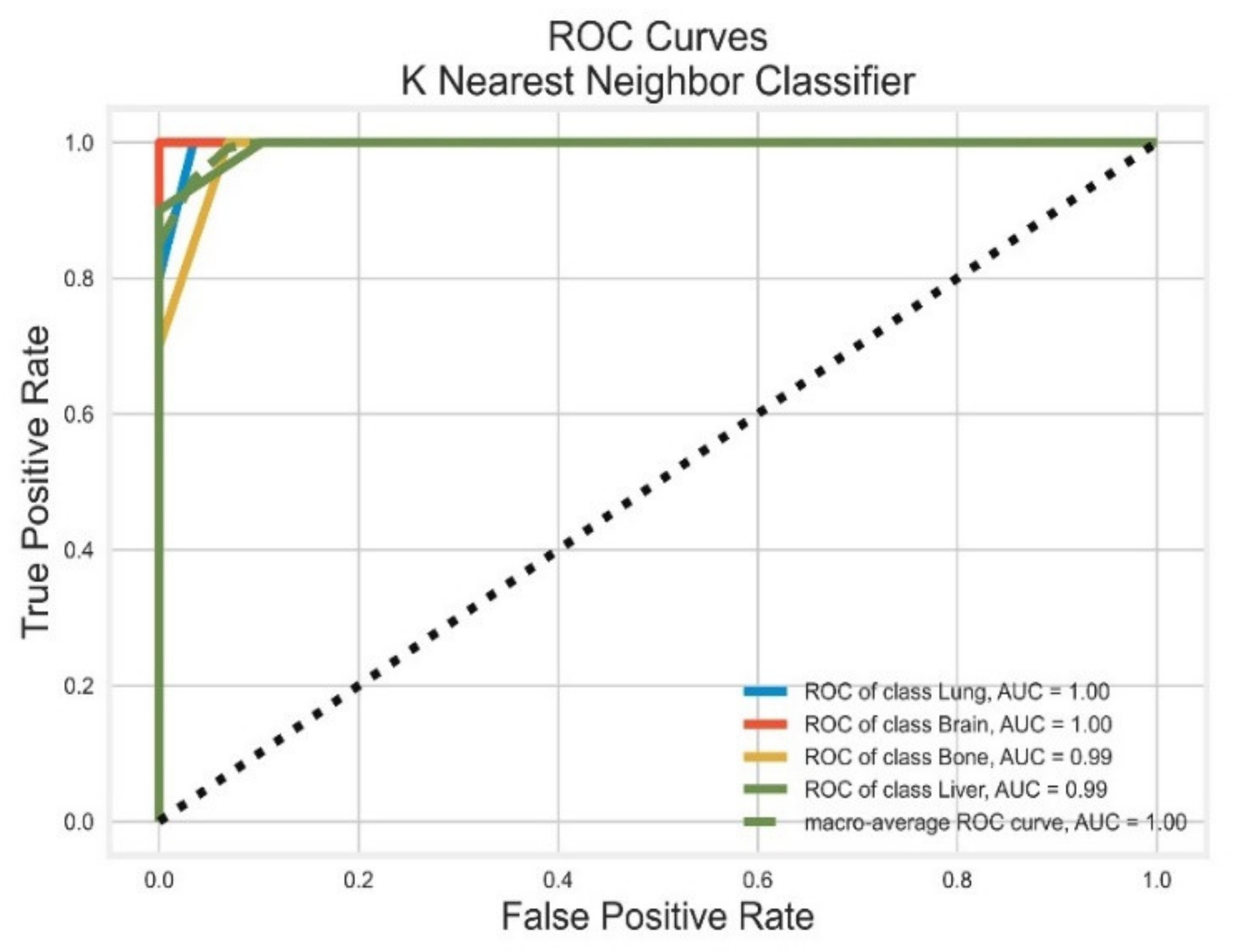
3.3. K-Nearest Neighbour Classifier

K-nearest neighbor classifier reported a training accuracy of 92% and validation or test accuracy of 87%. The confusion matrix depicted in Figure 21 indicates the misclassified samples. Out of 39 samples, five were misclassified with two samples from the lung class misclassified as liver and three samples from the bone class misclassified with one sample in each lung, brain, and liver class.
The classification report for the KNN classifier depicted in Figure 22 reveals the classifier’s overall performance. Class liver has low precision of 0.77 with low recall parameters of 0.7 and 0.8 for bone and lung classes, thus affecting the overall F1 score of these classes.
The precision-recall curve for the KNN classifier is calculated using one-vs-rest method as shown in Figure 23.
The KNN classifier had an average precision of 0.96, whereas all classes have PR AUC     0.95 , exhibiting a good classifier model. The Receiver Operator Characteristic (ROC) is shown below for the KNN classifier in Figure 24 using the one-vs-all method.
The average AUC = 1.0 for the KNN classifier model where all classes have an AUC     0.99 , the greater the value of AUC better is the separability among all classes.

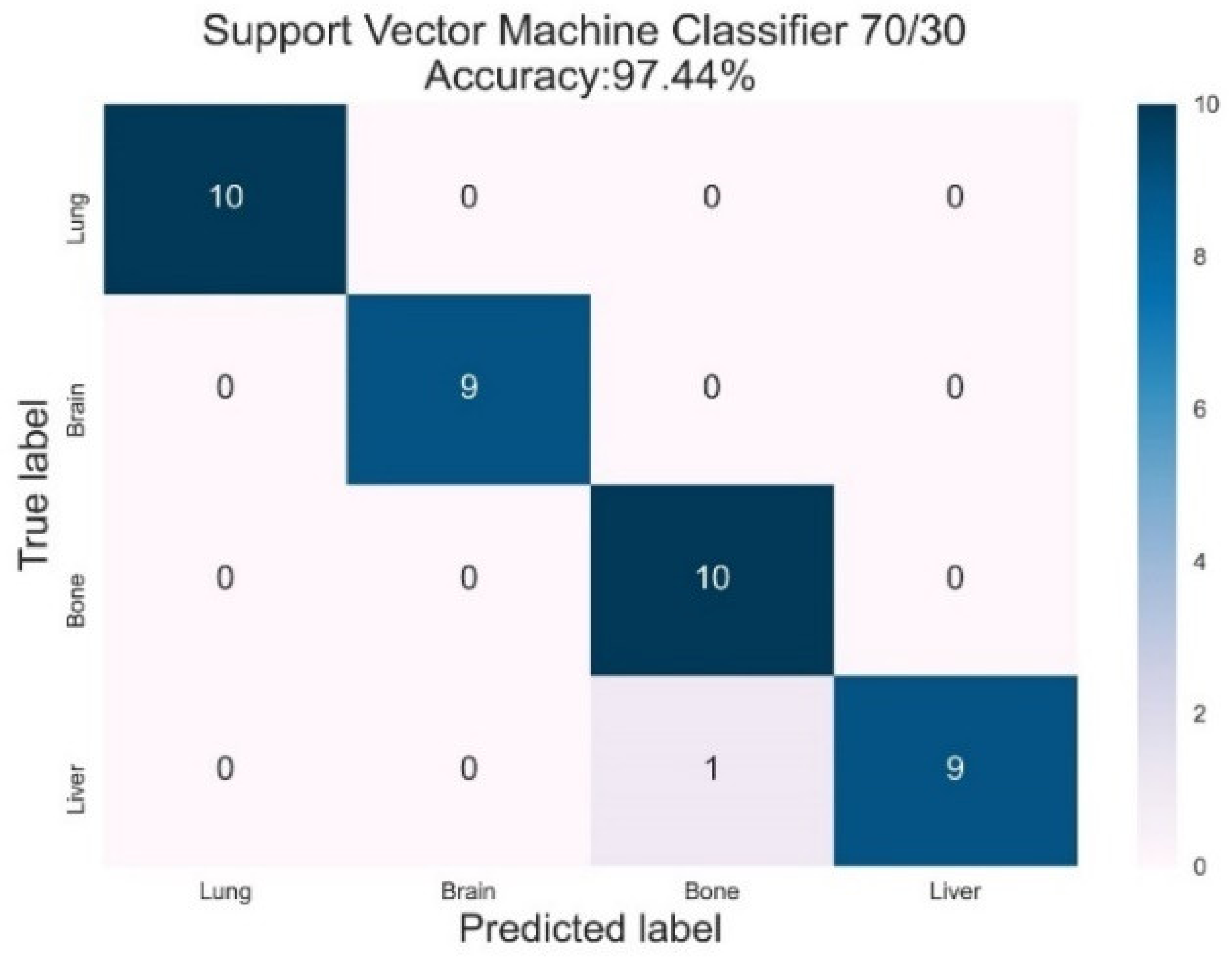
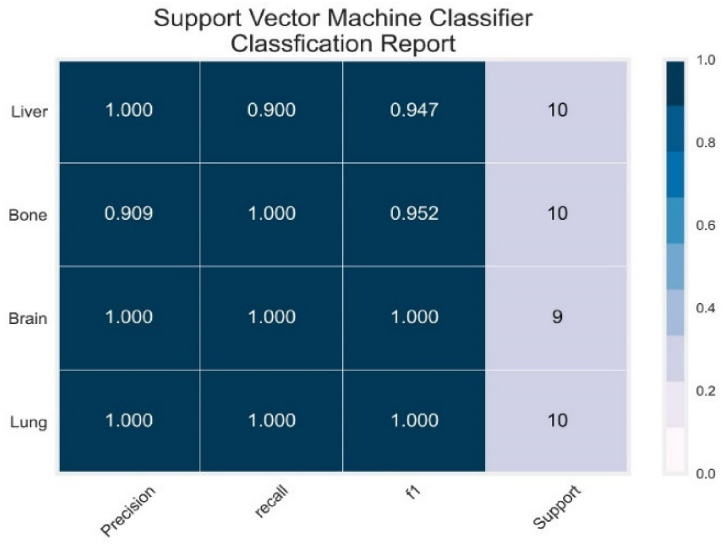
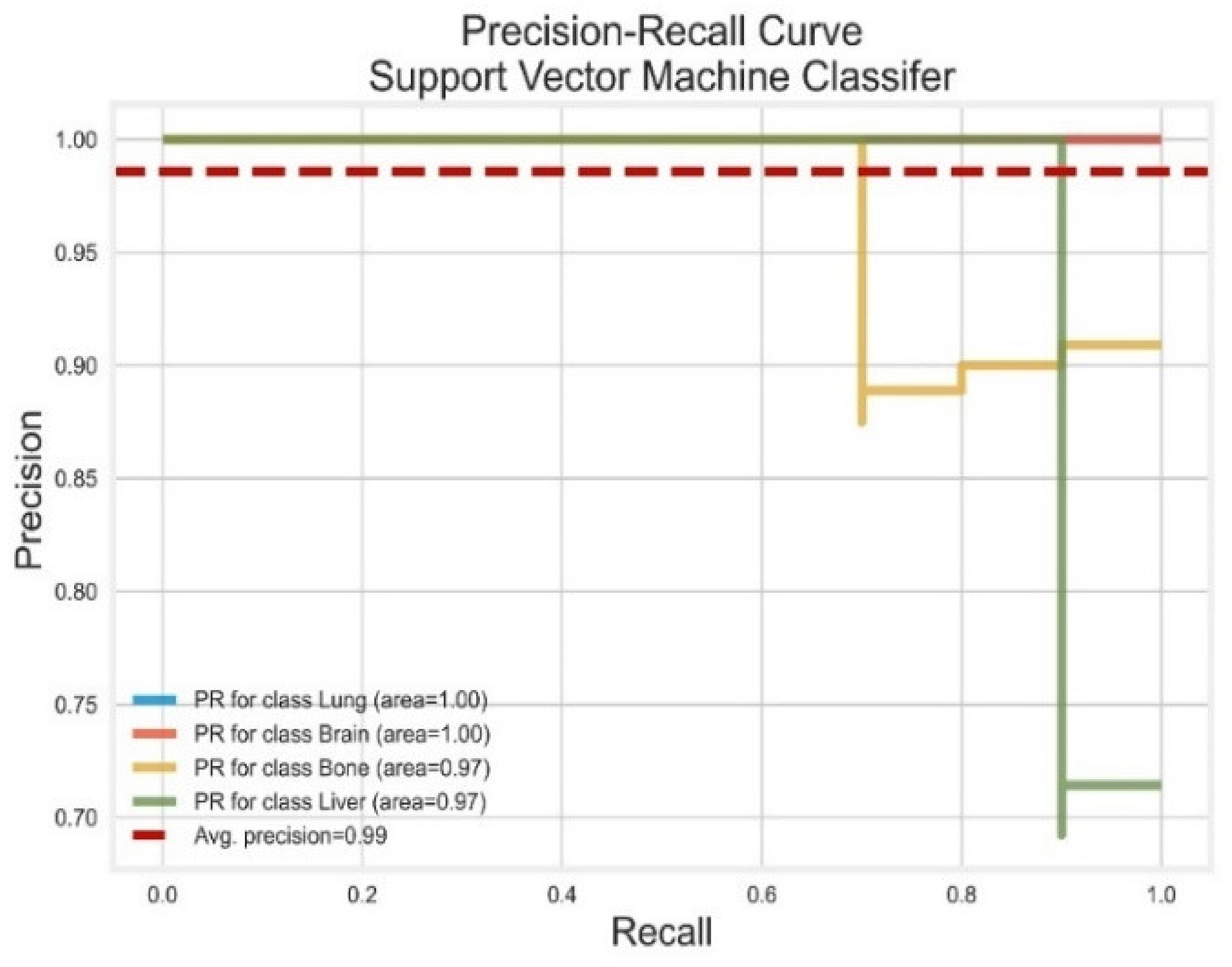
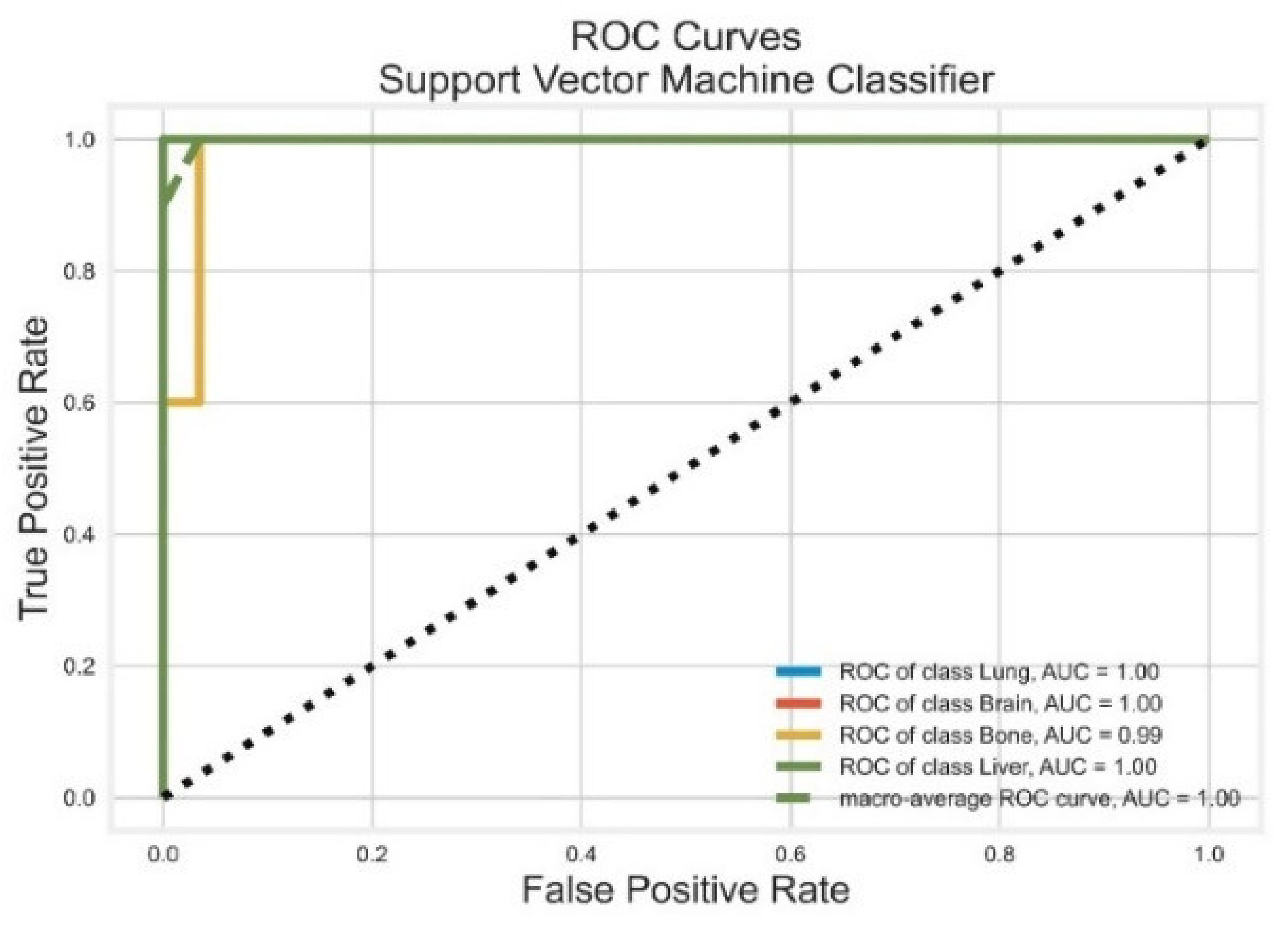
3.4. Support Vector Machines

The support vector machines classifier has shown excellent results with training accuracy of 100% and validation or test accuracy of 97%. The confusion matrix is depicted in Figure 25. Only one sample out of 39 samples is misclassified with one sample from the liver class reported under bone class.
The classification report for the SVM classifier visualized in Figure 26 revealed the excellent performance of the classifier. Precision and recall for all classes are 0.99   1.0 and thus has a very high F1 score for each class.
The precision-recall curve for the SVM classifier applying the one-vs-rest method is shown in Figure 27.
The SVM classifier has an excellent average precision of 0.99, whereas all classes have PR AUC     0.97 , exhibiting an outstanding classifier model. The Receiver Operator Characteristic (ROC) is shown below for SVM Classifier in Figure 28 using the one-vs-all method.
The average for the SVM classifier model is AUC = 1.0 where the bone class has an AUC = 0.99, while all other classes have an AUC = 1.0. SVM is the best classifier with maximum separability among all classes. A tabular comparison is shown in Table 3. All four different classifiers have been compared based on precision, recall, F1 score, PR–AUC, ROC–AUC, and the number of misclassified samples. The SVM Classifier has outperformed all other classifiers as it has high accuracy, low variance, higher precision, recall, and F1 score. Moreover, this classifier has the least misclassified samples and the highest PR–AUC ROC–AUC values per class. All the AUC presented for different classifiers have been calculated with 95% confidence interval and p > 0.05.
Nevertheless, significant results have been achieved. Further research is required to validate these models on diverse datasets. However, computation power is one of the most significant constraints in handling gene expression microarray datasets.

4. Conclusions

This paper concluded that breast cancer prognosis often metastasizes towards bones, liver, brain, and lungs; a leading cause of death in women. It uniquely integrated machine learning and microarrays for the identification of breast cancer using K-nearest neighbors, missing values are imputed, recursive feature elimination with cross-validation, and class imbalance is handled by employing K-means SMOTE. This work successfully identified the 16 most essential Entrez Gene IDs responsible for predicting metastatic locations in the bones, brain, liver, and lungs. Extensive experiments were conducted on NCBI Gene Expression Omnibus GSE14020 and GSE54323 datasets. Multiple classification models were considered, and results were presented by considering reliable matrices such as ROC–AUC and PR–AUC, and F1-score. In the future, the authors aim to extend this work using more advanced learning approaches on multiple large datasets to identify the different metastasis stages.

Author Contributions

Conceptualization, F.R. and F.A., methodology, I.U.D., A.A. and S.U.D.; software, F.R.; validation, F.A.; formal analysis, I.U.D. and B.-S.K.; investigation, A.A. and B.-S.K.; resources, B.-S.K.; data curation, F.R. and F.A.; writing—original draft preparation, F.R. and F.A., writing— review and editing, I.U.D. and A.A.; visualization, B.-S.K. and A.A.; supervision, S.U.D.; project administration, S.U.D.; funding acquisition, B.-S.K. All authors have read and agreed to the published version of the manuscript.

Funding

This work was supported in part by the National Research Foundation (NRF), Korea, under project BK21 FOUR (F21YY8102068); and in part by King Saud University, Riyadh, Saudi Arabia, through Researchers Supporting Project Number RSP-2022/184.

Conflicts of Interest

The authors declare no conflict of interest.

Abbreviations

AUCArea under the curve
BCBreast Cancer
BCBoMBreast Cancer Bone Metastasis
BCBrMBreast Cancer Brain Metastasis
BCLiMBreast Cancer Liver Metastasis
BCLuMBreast Cancer Lung Metastasis
CTCsCirculating Tumor cells
CV Cross validation
DTDecision Tree supervised learning algorithm
FNFalse Negative
FPFalse Positive
GEOGene expression omnibus
K-MeansUnsupervised learning algorithm that partition dataset into K number of clusters
KNNK-Nearest Neighbors supervised learning algorithm
NCBINational Center for Biotechnology Information
NRFNational Research Foundation
PRPrecision Recall
RFRandom Forrest supervised learning algorithm
RFECVRecursive Feature Elimination with cross validation
ROCReceiver operating characteristic curve
SMOTESynthetic object oversampling technique
SVMSupport Vector Machine supervised learning algorithm
TNTrue Negative
TPTrue Positive

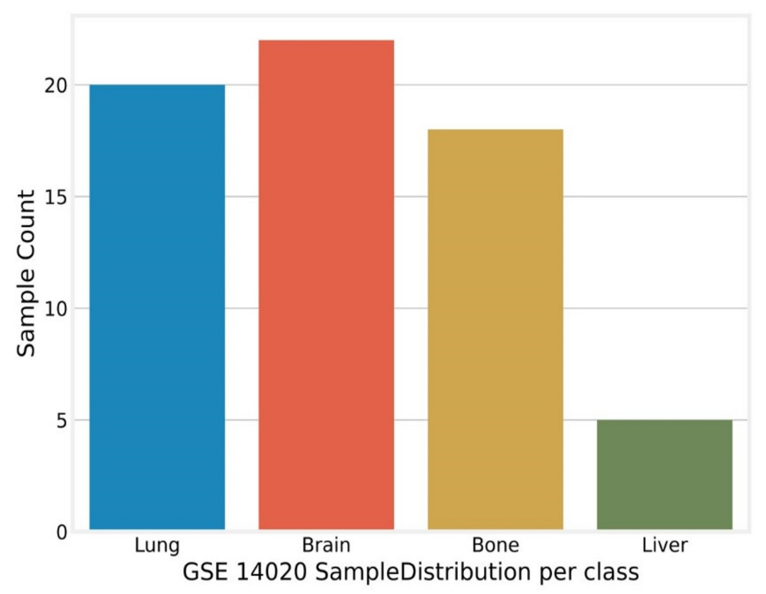
Appendix A. GSE14020

ENTREZ_GENE_IDIndex110100100010,000100,009,676999099919992999399949997Metastasis
0GSM3520958.23396.06837.88486.87216.69235.10575.26067.94406.48499.35386.573510.7023Lung
1GSM3520976.90536.84957.07989.16826.94915.31456.37467.68206.64598.75317.00918.8169Brain
2GSM3520987.71137.23296.54957.22436.27325.58235.92978.26166.56619.77867.642310.8695Brain
3GSM3521007.37706.70697.83927.31337.13245.10225.88557.64616.53358.98646.85019.6639Bone
4GSM3521017.45276.89926.453510.03036.49485.16455.72417.48006.70759.06877.07949.8207Brain
5GSM3521037.45286.82746.386610.81267.19715.40205.81367.37236.80728.37427.33509.8820Bone
6GSM3521057.81876.69379.457710.78176.63655.10326.16657.11276.60308.40567.455210.1645Bone
7GSM3521076.92456.41577.18587.81568.37125.06865.87527.55976.37308.81208.578210.5591Brain
8GSM3521097.37676.42977.11497.54146.65575.11515.74567.40646.36958.58746.99179.9465Bone
9GSM3521106.93556.84557.20188.05896.50795.27035.86819.37386.68259.01427.12299.2914Brain
55GSM352159NaN7.10896.69046.77845.1182NaN5.96077.04776.85787.48866.92338.5203Bone
56GSM352160NaN6.55737.51346.83055.4619NaN6.11376.72456.80117.82246.60209.0305Lung
57GSM352161NaN7.14616.91376.62665.0809NaN5.89236.56357.17018.32987.22579.5441Lung
58GSM352162NaN7.66706.47417.04525.1741NaN5.79486.66916.73817.56077.85977.8423Liver
59GSM352163NaN6.99497.48646.68445.5261NaN6.28906.75737.00707.55906.27279.0151Bone
60GSM352164NaN6.55127.33067.44195.4275NaN5.86706.28736.79038.05157.11168.6275Lung
61GSM352165NaN6.54407.33356.68735.9610NaN5.65636.97626.79838.16096.11139.2522Lung
62GSM352166NaN6.94976.69136.65066.2395NaN5.90616.23987.03677.80286.86718.4663Lung
63GSM352167NaN6.76767.13457.63196.5522NaN5.92336.58316.94598.04676.38938.5806Bone
64GSM352168NaN7.48836.90536.85125.6716NaN6.56216.04877.08217.71476.93709.2354Lung
65 rows × 20,488 columns.

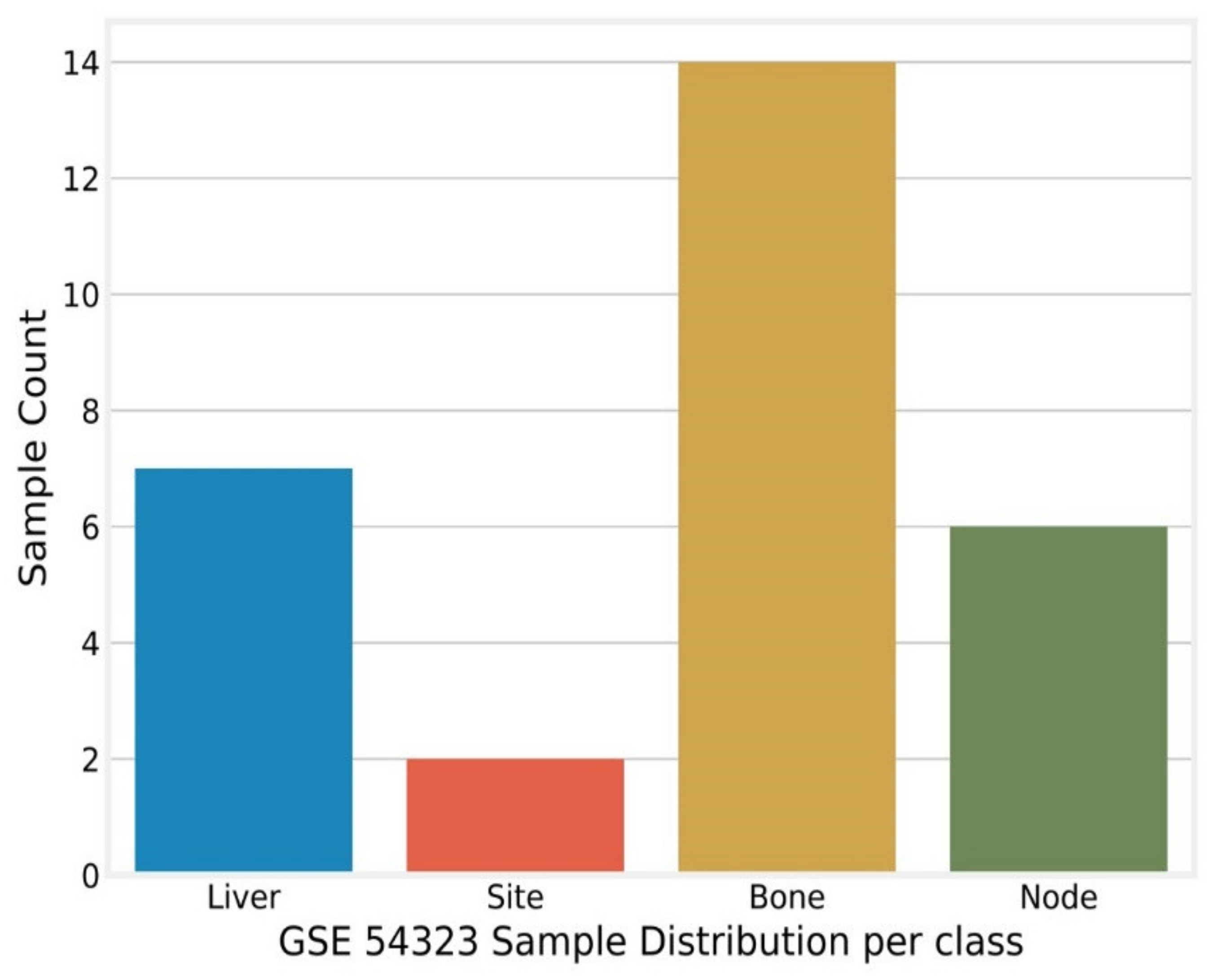
Appendix B. GSE54323

ENTREZ_GENE_IDIndex110100100010,000100,009,676999099919992999399949997Metastasis
0GSM13129287.56026.44697.33715.78044.42524.93106.48658.27515.98368.23466.80239.9452Liver
1GSM131292910.38858.28727.84237.37614.60255.11806.05576.94956.77548.01155.81849.1237Liver
2GSM13129306.71335.83665.79556.90654.64574.87815.45048.94696.31868.33716.33729.3204Site
3GSM13129316.21216.34395.70625.99184.35144.86266.34889.01946.42198.19646.246210.2259Site
4GSM13129325.80984.99866.99005.34024.60994.94935.23747.89076.18648.03676.015410.5537Bone
5GSM13129335.69225.03706.00005.35124.25504.90946.73748.41356.10858.26705.82289.6436Bone
6GSM13129346.21215.49787.27235.38444.34295.71495.94289.29406.22578.31656.63259.7894Node
7GSM13129356.40324.88217.35765.59755.34794.98066.11427.34876.16578.00866.47509.3352Node
8GSM13129366.53545.33536.25035.42794.34485.25405.51278.11446.29928.40496.38649.6644Node
9GSM13129376.19655.08687.09035.25494.96374.92616.86427.67837.07308.47425.446910.6389Node
19GSM13129476.01024.86737.45045.03225.01024.95728.38118.81056.27328.10656.253010.7216Bone
20GSM13129486.07445.09046.76795.72454.46324.79796.82978.10706.52808.11005.96238.9717Bone
21GSM13129496.70864.84076.60895.59504.34825.01146.96967.18996.31868.28585.66718.6960Bone
22GSM13129505.76945.50627.22075.21195.09365.32365.59298.31976.08608.15926.93279.4827Node
23GSM13129516.13435.44386.66835.50996.13555.58165.94908.37836.49968.34476.47869.3974Node
24GSM13129525.85634.85925.67575.32354.49935.28105.67948.81076.20948.18635.86038.3529Liver
25GSM13129538.84996.04985.99156.10304.36045.00265.35458.19706.27798.23105.95609.5760Bone
26GSM13129546.31374.76535.18425.21774.23255.73085.27669.36916.13718.01646.10848.2146Bone
27GSM13129555.99515.05176.41635.26824.37454.89836.22878.70486.06698.49425.68149.5736Bone
28GSM13129566.05454.71726.95085.19124.37654.87797.69658.83766.44318.20286.56849.2403Bone
29 rows × 20,488 columns.

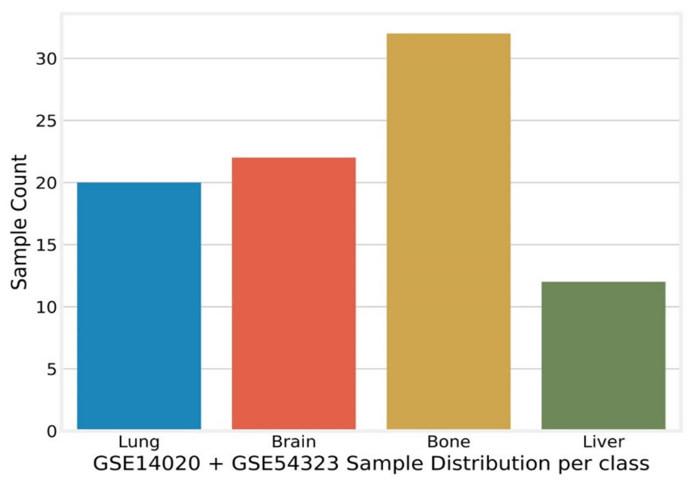
Appendix C. Merged and Normalized Dataset

1101001000100001 × 10810001...999999099919992999399949997
01.1073−0.55841.4254−0.16790.968−0.71030.3433...0.235−1.40550.6487−0.7894 1.7514 −0.47 1.4987
1−0.40060.37140.20921.76041.23830.27660.7643...0.58230.53410.3564−0.2172 0.7292 0.1851 −0.5383
20.51420.8277−0.59210.12790.5271.54290.784...1.3263−0.24051.0032−0.5009 2.4741 1.1371 1.6794
30.13480.20171.35650.20271.4312−0.72691.0486...0.8783−0.31740.3164−0.6167 1.1261 −0.0541 0.3768
40.22060.4306−0.73712.48440.7602−0.43211.08...0.8878−0.59840.1310.002 1.2663 0.2907 0.5462
50.22080.3451−0.83813.14131.49920.69061.4515...−3.5736−0.44260.01080.3564 0.0845 0.6751 0.6125
60.63610.1863.80183.11540.9093−0.72192.3365...−3.19120.1717−0.2788−0.3698 0.138 0.8558 0.9176
7−0.3789−0.1450.36930.62452.7348−0.88561.0825...1.0557−0.33540.2199−1.1873 0.8295 2.5444 1.3439
80.1344−0.12820.26220.39420.9295−0.6661.3149...0.9476−0.5610.0489−1.1998 0.4473 0.1588 0.6821
9−0.36640.36660.39350.82880.7740.06780.6543...2.0178−0.34772.2444−0.087 1.1735 0.3561 −0.0257
....................................... ... ... ...
76−1.6765−2.11170.5075−1.1132−0.8302−2.4271−1.1618...−0.80852.8795−0.3754−1.3423 −0.3784 −1.3842 1.1868
77−1.7519−1.7871−0.2358−1.4794−0.1956−0.0349−1.4196...−0.69192.61521.5135−1.5502 −0.057 −0.3818 0.9789
78−1.4165−1.98770.7691−1.713−0.8021−1.4121−0.6681...−1.10264.02751.6157−1.5423 −0.371 −0.952 1.5195
79−1.3437−1.7222−0.2621−1.1316−1.3777−2.1654−1.7002...−0.93861.32650.8307−0.6363 −0.365 −1.389 −0.3711
80−0.6238−2.0195−0.5024−1.2403−1.4987−1.1558−1.9665...−0.79431.5701−0.1927−1.3807 −0.0658 −1.8329 −0.6689
81−1.5912−1.9974−1.9121−1.4683−1.33970.1184−1.0834...0.0965−0.67621.616−1.7688 −0.2352 −1.5423 −1.0397
821.8065−0.5804−1.4351−0.8137−1.4859−1.1977−1.0668...0.8924−1.24190.9312−1.5253 −0.1591 −1.3984 0.2818
83−1.0721−2.1091−2.6548−1.5571−1.62052.2447−0.0992...0.7633−1.37752.2391−2.0259 −0.5243 −1.1693 −1.1891
84−1.4337−1.7683−0.7933−1.5147−1.4711−1.6908−1.2391...0.17580.28011.4978−2.2756 0.2887 −1.8114 0.2792
85−1.3663−2.16640.0143−1.5794−1.4689−1.7872−1.4259...−1.37312.83561.646−0.938 −0.207 −0.4777 −0.0809
86 rows × 20,486 columns.

Appendix D. Dataset after Removing Correlated Features

110100100010,0001 × 10810,00199619962997997399849999997
01.1073−0.55841.4254−0.16790.968−0.71030.34330.27060.45511.65661.1436−0.40510.2351.4987
1−0.40060.37140.20921.76041.23830.27660.76430.49080.41331.32210.6164−0.28040.5823−0.5383
20.51420.8277−0.59210.12790.5271.54290.7841.16410.41410.69740.92850.25041.32631.6794
30.13480.20171.35650.20271.4312−0.72691.04861.7457−0.34790.01110.5555−1.31930.87830.3768
40.22060.4306−0.73712.48440.7602−0.43211.081.4034−0.67570.86950.29263.61070.88780.5462
50.22080.3451−0.83813.14131.49920.69061.45150.17240.5311−0.2760.48350.33−3.57360.6125
60.63610.1863.80183.11540.9093−0.72192.33650.32190.6182−0.45910.0423−0.6683−3.19120.9176
7−0.3789−0.1450.36930.62452.7348−0.88561.08250.0195−0.1824−0.33092.046−0.00841.05571.3439
80.1344−0.12820.26220.39420.9295−0.6661.31490.9737−0.5723−0.60660.7488−0.13130.94760.6821
9−0.36640.36660.39350.82880.7740.06780.65430.37070.2210.29250.1104−0.29572.0178−0.0257
76−1.6765−2.11170.5075−1.1132−0.8302−2.4271−1.1618−0.1819−1.91792.440.735−0.7166−0.80851.1868
77−1.7519−1.7871−0.2358−1.4794−0.1956−0.0349−1.41960.0729−0.4649−2.2167−2.49311.0378−0.69190.9789
78−1.4165−1.98770.7691−1.713−0.8021−1.4121−0.66810.9578−0.3947−1.3783−1.69170.2525−1.10261.5195
79−1.3437−1.7222−0.2621−1.1316−1.3777−2.1654−1.70020.1721−1.52571.3317−1.02510.5284−0.9386−0.3711
80−0.6238−2.0195−0.5024−1.2403−1.4987−1.1558−1.96650.5117−1.61212.2701−0.60820.2498−0.7943−0.6689
81−1.5912−1.9974−1.9121−1.4683−1.33970.1184−1.0834−0.0482−1.9324−0.947−1.64120.34560.0965−1.0397
821.8065−0.5804−1.4351−0.8137−1.4859−1.1977−1.06680.23920.4666−0.41422.40510.48090.89240.2818
83−1.0721−2.1091−2.6548−1.5571−1.62052.2447−0.0992−0.4106−1.118−2.1279−1.58750.44010.7633−1.1891
84−1.4337−1.7683−0.7933−1.5147−1.4711−1.6908−1.2391−1.3745−2.1706−0.6876−0.86331.34870.17580.2792
85−1.3663−2.16640.0143−1.5794−1.4689−1.7872−1.42590.2409−2.37950.45−0.25790.5958−1.3731−0.0809
86 rows × 6602 columns.

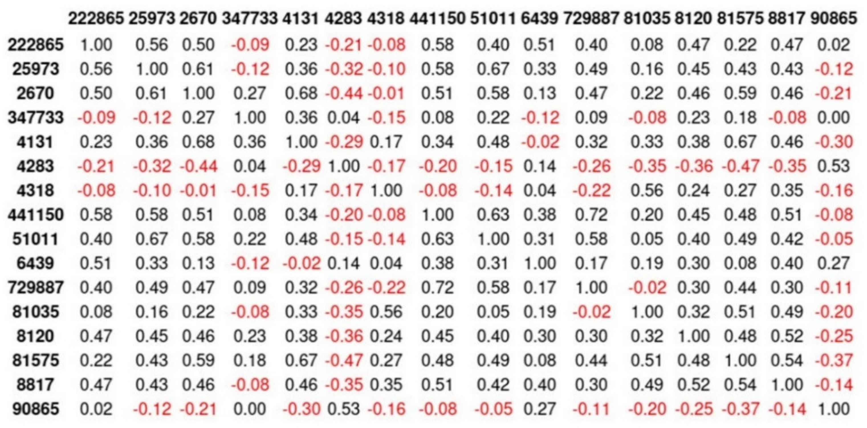
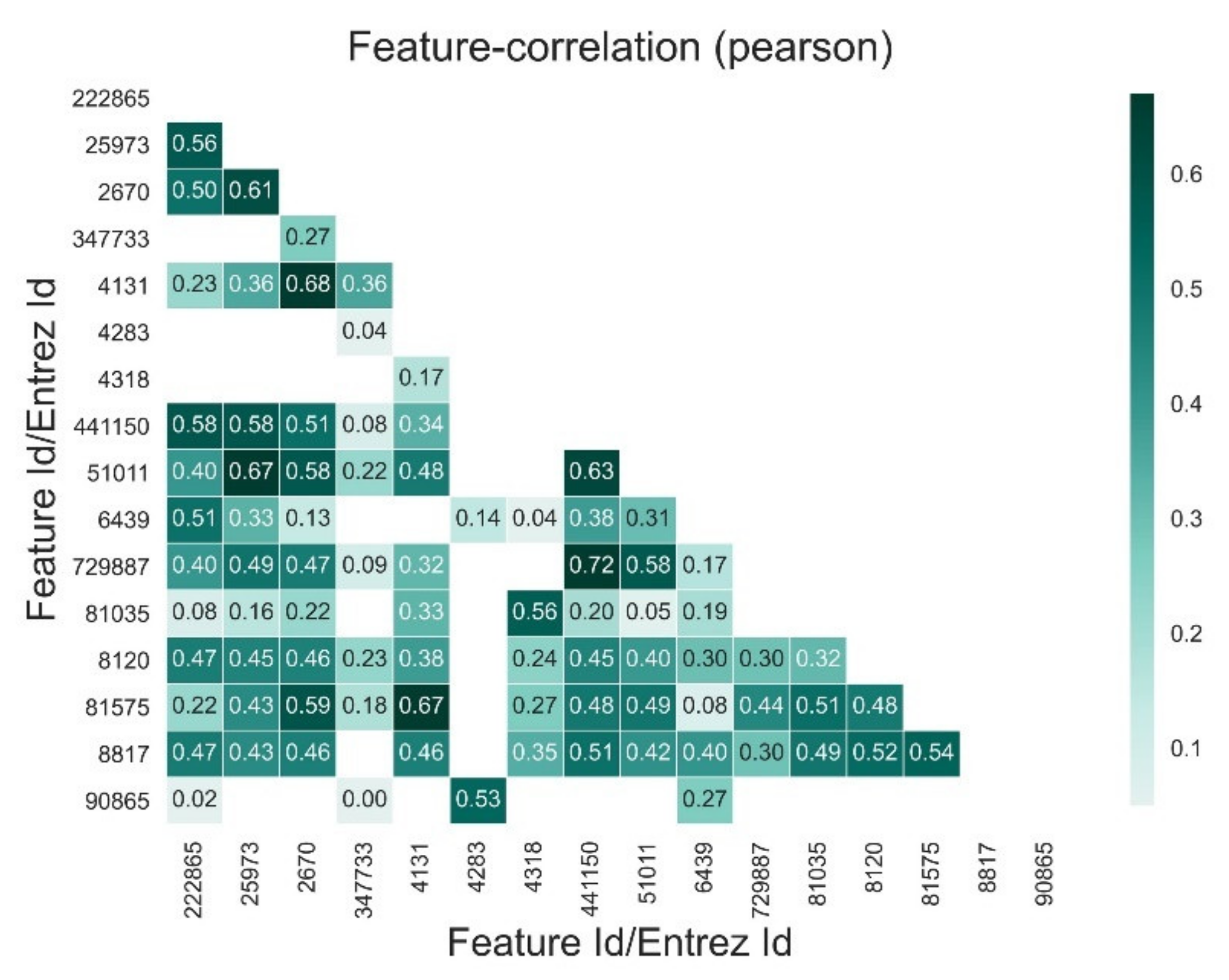
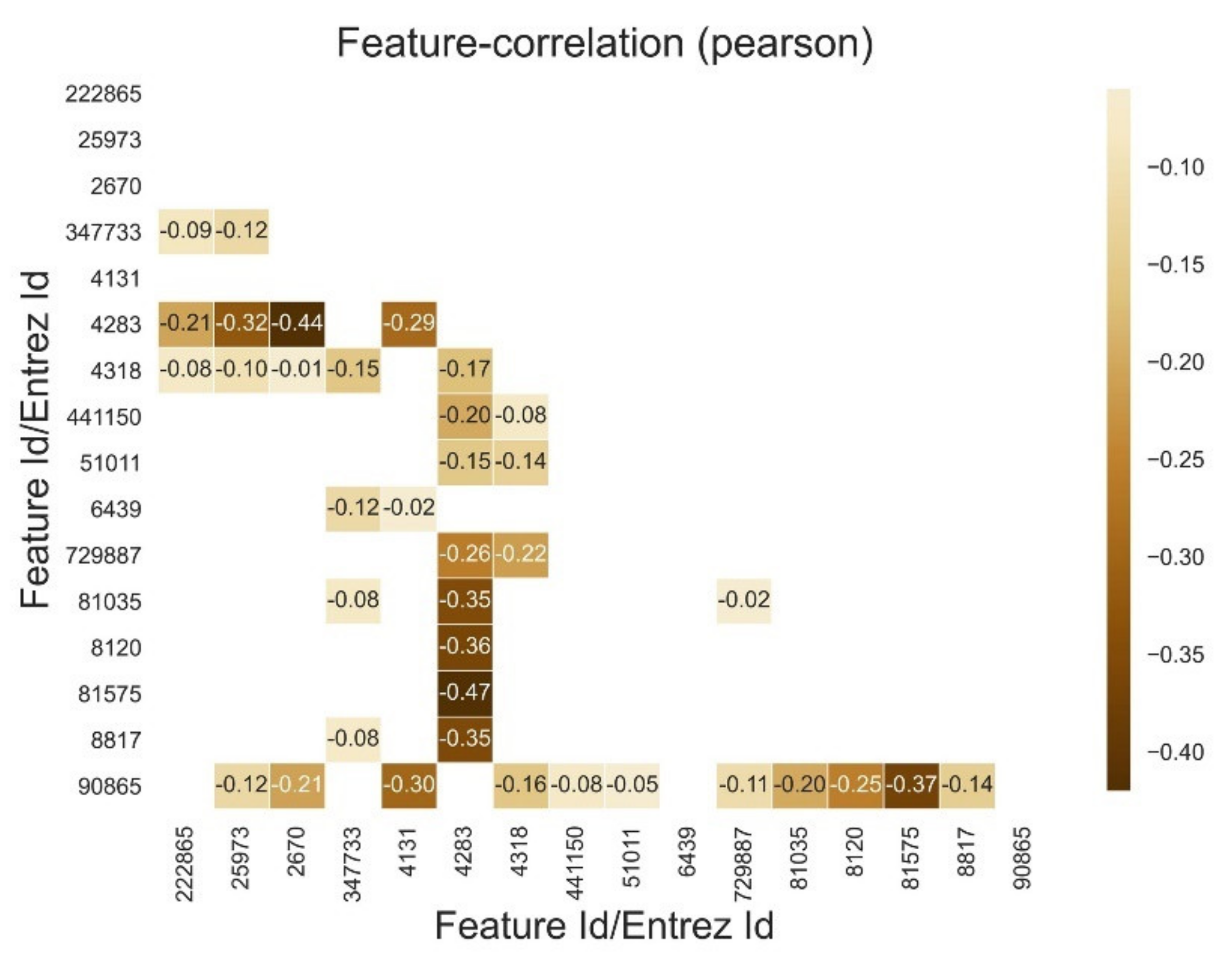
Appendix E. Reduced Dimensions after RFECV

222,86525,9732670347,733413142834318441,15051,0116439729,88781,035812081,575881790,865
00.1980.97580.3665−0.26961.04580.9783−0.64443.7823.1710.38324.6323−0.4311−0.2163−0.1137−0.12950.7515
1−0.08651.10.78643.3121.24160.53050.92940.61430.91980.1937−0.1079−0.38114.30881.2101−0.2767−0.4483
21.96461.12331.0511−0.08540.9364−0.79−1.20650.93560.1308−0.07362.1−0.710.27950.9134−0.3304−0.142
3−1.192−0.63670.2691−0.45621.7566−0.78461.4329−0.70150.4727−0.1349−0.77711.5955−0.32882.67313.88831.3303
40.1266−0.06041.71960.03981.8735−0.6590.02210.10350.4401−0.02722.0996−0.2556−0.4302−0.05810.8987−0.5004
5−0.59060.34911.42480.20062.0667−0.7052−0.5249−0.2215−0.33930.1466−0.89440.6907−0.2445−0.2771−0.0903−0.4262
6−0.88710.10410.1751−0.70431.6466−0.30170.1538−0.48970.40020.0265−0.43330.4794−0.06861.0238−0.2101−0.2477
70.44810.06210.99341.11761.0911−0.72030.09151.79541.4472−0.01972.5998−0.3057−0.53381.89070.3507−0.4034
8−0.20631.01180.0792−0.71381.03691.43411.8265−0.20830.2059−0.0171−0.85521.9019−0.50760.8470.28760.1463
9−0.27311.1552.07041.02022.5062−0.6621−0.5338−0.12180.76850.15530.1663−0.5509−0.20451.52890.1918−0.2485
76−1.012−1.9397−1.1871−0.9757−1.8074−0.54851.1886−1.6693−1.1848−0.9253−0.8543−0.6911−0.4686−0.2061−1.3553−0.7851
77−1.9576−0.0641−1.302−0.78030.17770.65411.6583−1.4042−0.9199−0.9623−1.6590.5504−0.8571−0.2125−1.4715−1.1276
78−1.786−1.2262−1.3476−0.3278−0.49010.59511.933−1.0345−1.1996−0.9378−1.89621.3793−0.8242−0.7745−1.7589−0.9362
79−0.2186−1.1662−1.15−0.7646−0.3131−1.30091.7065−2.237−1.5943−0.9207−0.95060.7116−0.90040.2218−1.887−1.096
801.0808−0.597−0.8584−0.8226−1.4641−1.23740.7571−1.4812−2.0239−0.7141−1.40480.3666−0.9214−1.35470.2259−1.0798
81−1.36240.1524−1.1858−0.8277−1.4117−1.2232−1.2171−0.8709−0.8319−0.8716−0.62821.7031−1.7363−0.7022−1.9667−1.0593
82−1.2753−0.6617−1.2841−0.67230.23540.0003−1.3449−0.3184−0.8008−0.85810.298−1.1678−0.6246−0.31641.769−0.4109
83−1.07550.189−1.3647−0.902−1.5986−1.9597−0.8797−1.0385−0.5315−0.7335−0.81411.275−1.888−0.2927−1.5776−1.1293
84−1.8085−1.0142−1.2811−0.9334−1.0717−0.43230.9235−2.1046−1.0034−0.9462−0.8141−1.2629−0.9565−0.2507−1.7703−0.6834
85−0.6364−1.8746−0.8828−0.8022−1.99140.12441.8855−1.3999−1.2799−0.7505−0.6868−1.4617−0.0416−1.7382−1.2005−0.5755
86 rows × 16 columns.

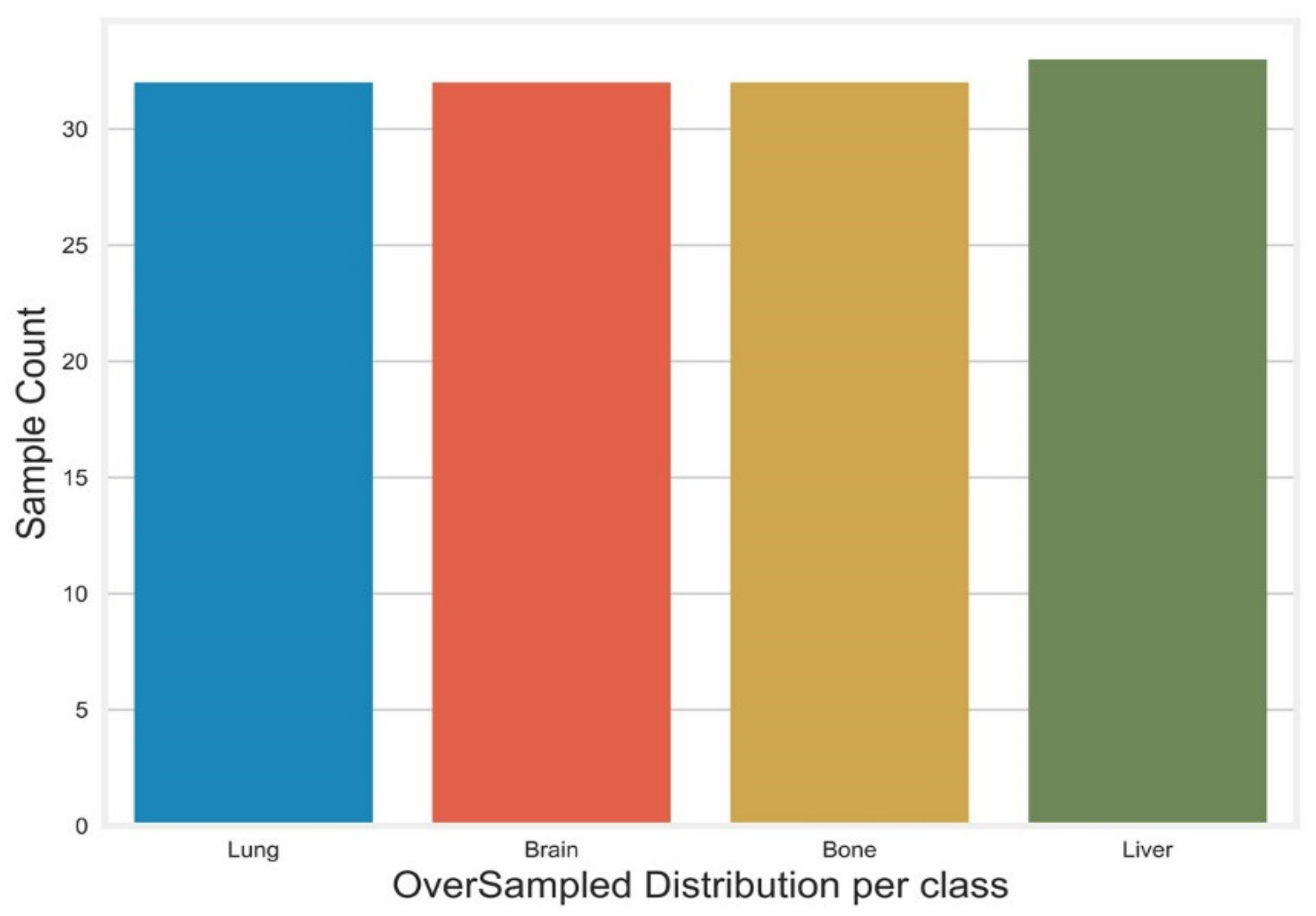
Appendix F. Oversampled Dataset after Applying K-Mean Smote

222,86525,9732670347,733413142834318441,15051,0116439729,88781,035812081,575881790,865Metastasis
00.1980.97580.3665−0.26961.04580.9783−0.64443.7823.1710.38324.6323−0.4311−0.2163−0.1137−0.12950.7515Lung
1−0.08651.10.78643.3121.24160.53050.92940.61430.91980.1937−0.1079−0.38114.30881.2101−0.2767−0.4483Brain
21.96461.12331.0511−0.08540.9364−0.79−1.20650.93560.1308−0.07362.1−0.710.27950.9134−0.3304−0.142Brain
3−1.192−0.63670.2691−0.45621.7566−0.78461.4329−0.70150.4727−0.1349−0.77711.5955−0.32882.67313.88831.3303Bone
40.1266−0.06041.71960.03981.8735−0.6590.02210.10350.4401−0.02722.0996−0.2556−0.4302−0.05810.8987−0.5004Brain
5−0.59060.34911.42480.20062.0667−0.7052−0.5249−0.2215−0.33930.1466−0.89440.6907−0.2445−0.2771−0.0903−0.4262Bone
6−0.88710.10410.1751−0.70431.6466−0.30170.1538−0.48970.40020.0265−0.43330.4794−0.06861.0238−0.2101−0.2477Bone
70.44810.06210.99341.11761.0911−0.72030.09151.79541.4472−0.01972.5998−0.3057−0.53381.89070.3507−0.4034Brain
8−0.20631.01180.0792−0.71381.03691.43411.8265−0.20830.2059−0.0171−0.85521.9019−0.50760.8470.28760.1463Bone
9−0.27311.1552.07041.02022.5062−0.6621−0.5338−0.12180.76850.15530.1663−0.5509−0.20451.52890.1918−0.2485Brain
119−1.2187−2.5334−1.3281.6502−0.18682.3117−0.7413−1.161−0.9107−0.8275−0.8525−0.9858−1.3184−1.3744−1.95710.8591Liver
120−0.9832−1.4084−1.0220.3152−1.21421.989−0.7787−1.2526−0.7445−0.5679−0.9831−1.2853−1.8635−1.9452−1.54833.7285Liver
121−1.4467−1.1812−1.33960.4043−0.93981.6933−1.1969−1.693−0.9057−0.8883−1.0399−1.4553−1.4607−2.0827−2.21890.1661Liver
122−0.5328−1.365−0.97571.0245−0.92612.2429−0.9658−1.1536−0.8336−0.5485−0.9617−1.2656−1.912−2.0633−1.21533.7183Liver
123−0.7801−1.3888−1.00110.6352−1.08422.1035−0.8631−1.2079−0.7847−0.5592−0.9735−1.2764−1.8854−1.9984−1.3983.7239Liver
124−1.1877−0.5688−1.1857−0.0131−1.34371.6019−1.3146−1.7328−0.8642−0.7686−1.1032−1.614−1.7331−2.4309−1.92831.4033Liver
125−1.331−2.2994−1.27691.0944−0.52032.1472−0.6812−1.2176−0.8412−0.7769−0.8893−1.0595−1.4218−1.458−1.9881.5002Liver
126−1.0673−2.7155−1.36282.1930.12032.4782−0.815−1.1022−0.9786−0.8655−0.8199−0.9239−1.2419−1.3232−1.88720.3424Liver
127−1.5902−0.5177−1.3223−0.3542−1.39721.3651−1.3603−1.9386−0.8735−0.8917−1.1338−1.6824−1.5646−2.4134−2.34120.1555Liver
128−1.7172−1.307−1.126−0.8419−1.68351.5209−0.5981−1.5013−0.6315−0.638−1.0401−1.3814−1.7628−1.8607−2.13683.2783Liver
129 rows × 17 columns.

References

  1. Medeiros, B.; Allan, A.L. Molecular Mechanisms of Breast Cancer Metastasis to the Lung: Clinical and Experimental Perspectives. Int. J. Mol. Sci. 2019, 20, 2272. [Google Scholar] [CrossRef] [PubMed] [Green Version]
  2. Chaffer, C.L.; Weinberg, R.A. A Perspective on Cancer Cell Metastasis. Science 2011, 331, 1559–1564. [Google Scholar] [CrossRef] [PubMed]
  3. JPMA—Journal of Pakistan Medical Association. Available online: https://jpma.org.pk/article-details/1863 (accessed on 13 February 2021).
  4. Menhas, R.; Umer, S. Breast Cancer among Pakistani Women. Iran. J. Public Health 2015, 44, 586–587. [Google Scholar] [PubMed]
  5. Zaheer, S.; Shah, N.; Maqbool, S.A.; Soomro, N.M. Estimates of Past and Future Time Trends in Age-Specific Breast Cancer Incidence among Women in Karachi, Pakistan: 2004–2025. BMC Public Health 2019, 19, 1001. [Google Scholar] [CrossRef]
  6. Lambert, A.W.; Pattabiraman, D.R.; Weinberg, R.A. Emerging Biological Principles of Metastasis. Cell 2017, 168, 670–691. [Google Scholar] [CrossRef] [Green Version]
  7. Hess, K.R.; Varadhachary, G.R.; Taylor, S.H.; Wei, W.; Raber, M.N.; Lenzi, R.; Abbruzzese, J.L. Metastatic Patterns in Adenocarcinoma. Cancer 2006, 106, 1624–1633. [Google Scholar] [CrossRef]
  8. Wu, Q.; Li, J.; Zhu, S.; Wu, J.; Chen, C.; Liu, Q.; Wei, W.; Zhang, Y.; Sun, S. Breast Cancer Subtypes Predict the Preferential Site of Distant Metastases: A SEER Based Study. Oncotarget 2017, 8, 27990–27996. [Google Scholar] [CrossRef] [Green Version]
  9. Schlappack, O.K.; Baur, M.; Steger, G.; Dittrich, C.; Moser, K. The Clinical Course of Lung Metastases from Breast Cancer. Klin. Wochenschr. 1988, 66, 790–795. [Google Scholar] [CrossRef]
  10. Xiao, W.; Zheng, S.; Liu, P.; Zou, Y.; Xie, X.; Yu, P.; Tang, H.; Xie, X. Risk Factors and Survival Outcomes in Patients with Breast Cancer and Lung Metastasis: A Population-Based Study. Cancer Med. 2018, 7, 922–930. [Google Scholar] [CrossRef]
  11. GSE14020—NCBI. Available online: https://www.ncbi.nlm.nih.gov/search/all/?term=GSE14020 (accessed on 6 December 2020).
  12. GSE54323—NCBI. Available online: https://www.ncbi.nlm.nih.gov/search/all/?term=GSE54323 (accessed on 6 December 2020).
  13. Daoud, M.; Mayo, M. A Survey of Neural Network-Based Cancer Prediction Models from Microarray Data. Artif. Intell. Med. 2019, 97, 204–214. [Google Scholar] [CrossRef]
  14. Yazici, H.; Akin, B. Molecular Genetics of Metastatic Breast Cancer. In Tumour Progression and Metastasis; 2020; Available online: https://books.google.com.hk/books?hl=zh-CN&lr=&id=WXL8DwAAQBAJ&oi=fnd&pg=PA33&dq=Molecular+Genetics+of+Metastatic+Breast+Cancer.+In+Tumou&ots=fD07Myo0Zn&sig=N7UQpRfEosuIQxpTXI4KZx755Yc&redir_esc=y&hl=zh-CN&sourceid=cndr#v=onepage&q=Molecular%20Genetics%20of%20Metastatic%20Breast%20Cancer.%20In%20Tumou&f=false (accessed on 10 June 2022).
  15. Saunus, J.M.; Momeny, M.; Simpson, P.T.; Lakhani, S.R.; Da Silva, L. Molecular Aspects of Breast Cancer Metastasis to the Brain. Genet. Res. Int. 2011, 2011, 1–9. [Google Scholar] [CrossRef] [Green Version]
  16. Jin, X.; Mu, P. Targeting Breast Cancer Metastasis. Breast Cancer Basic Clin. Res. 2015, 9, 23–34. [Google Scholar] [CrossRef] [Green Version]
  17. Macedo, F.; Ladeira, K.; Pinho, F.; Saraiva, N.; Bonito, N.; Pinto, L.; Gonçalves, F. Bone Metastases: An Overview. Oncol. Rev. 2017, 11, 321. [Google Scholar] [CrossRef]
  18. Ma, R.; Feng, Y.; Lin, S.; Chen, J.; Lin, H.; Liang, X.; Zheng, H.; Cai, X. Mechanisms Involved in Breast Cancer Liver Metastasis. J. Transl. Med. 2015, 13, 64. [Google Scholar] [CrossRef] [Green Version]
  19. Zhao, H.Y.; Gong, Y.; Ye, F.G.; Ling, H.; Hu, X. Incidence and Prognostic Factors of Patients with Synchronous Liver Metastases upon Initial Diagnosis of Breast Cancer: A Population-Based Study. Cancer Manag. Res. 2018, 10, 5937–5950. [Google Scholar] [CrossRef] [Green Version]
  20. Pedrosa, R.M.S.M.; Mustafa, D.A.; Soffietti, R.; Kros, J.M. Breast Cancer Brain Metastasis: Molecular Mechanisms and Directions for Treatment. Neuro. Oncol. 2018, 20, 1439–1449. [Google Scholar] [CrossRef]
  21. Brosnan, E.M.; Anders, C.K. Understanding Patterns of Brain Metastasis in Breast Cancer and Designing Rational Therapeutic Strategies. Ann. Transl. Med. 2018, 6, 163. [Google Scholar] [CrossRef]
  22. Stella, G.M.; Kolling, S.; Benvenuti, S.; Bortolotto, C. Lung-Seeking Metastases. Cancers 2019, 11, 1010. [Google Scholar] [CrossRef] [Green Version]
  23. Jin, L.; Han, B.; Siegel, E.; Cui, Y.; Giuliano, A.; Cui, X. Breast Cancer Lung Metastasis: Molecular Biology and Therapeutic Implications. Cancer Biol. Ther. 2018, 19, 858–868. [Google Scholar] [CrossRef] [Green Version]
  24. Edgar, R.; Domrachev, M.; Lash, A.E. Gene Expression Omnibus: NCBI Gene Expression and Hybridization Array Data Repository. Nucleic Acids Res. 2002, 30, 207–210. [Google Scholar] [CrossRef] [Green Version]
  25. Affimetrix Human Genome U133 Arrays the Most Comprehensive Coverage of the Human Genome in Two Flexible Formats: Single-Array Cartridges and Multi-Array Plates; 2017; Available online: https://www.thermofisher.com/ (accessed on 1 January 2022).
  26. Maglott, D.; Ostell, J.; Pruitt, K.D.; Tatusova, T. Entrez Gene: Gene-Centered Information at NCBI. Nucleic Acids Res. 2011, 39. [Google Scholar] [CrossRef]
  27. SOFT—GEO—NCBI. Available online: https://www.ncbi.nlm.nih.gov/geo/info/soft.html (accessed on 2 January 2021).
  28. GEOparse—GEOparse 1.2.0 Documentation. Available online: https://geoparse.readthedocs.io/en/latest/introduction.html (accessed on 19 December 2020).
  29. Liew, A.W.-C.; Law, N.-F.; Yan, H. Missing Value Imputation for Gene Expression Data: Computational Techniques to Recover Missing Data from Available Information. Brief. Bioinform. 2011, 12, 498–513. [Google Scholar] [CrossRef] [Green Version]
  30. Bonaccorso, G. Machine Learning Algorithms: A Reference Guide to Popular Algorithms for Data Science and Machine Learning; Packt Publishing: Birmingham, UK, 2017; ISBN 1785889621. [Google Scholar]
  31. Lin, W.C.; Tsai, C.F. Missing Value Imputation: A Review and Analysis of the Literature (2006–2017). Artif. Intell. Rev. 2020, 53, 1487–1509. [Google Scholar] [CrossRef]
  32. Troyanskaya, O.; Cantor, M.; Sherlock, G.; Brown, P.; Hastie, T.; Tibshirani, R.; Botstein, D.; Altman, R.B. Missing Value Estimation Methods for DNA Microarrays. Bioinformatics 2001, 17, 520–525. [Google Scholar] [CrossRef] [PubMed] [Green Version]
  33. Hastie, T.; Tibshirani, R.; Sherlock, G.; Eisen, M.; Brown, P.; Botstein, D. Imputing Missing Data for Gene Expression Arrays. Stanford Univ. Stat. Dep. Tech. Rep. 2006, 3, 27. Available online: http://www.stat.stanford.edu/Hast.pdf/cll/qxd. (accessed on 2 January 2021).
  34. Sklearn.Impute.KNNImputer—Scikit-Learn 0.24.0 Documentation. Available online: https://scikit-learn.org/stable/modules/generated/sklearn.impute.KNNImputer.html (accessed on 8 January 2021).
  35. Dash, R.; Misra, B.B. Performance Analysis of Clustering Techniques over Microarray Data: A Case Study. Phys. A Stat. Mech. Its Appl. 2018, 493, 162–176. [Google Scholar] [CrossRef]
  36. Mukaka, M.M. Statistics Corner: A Guide to Appropriate Use of Correlation Coefficient in Medical Research. Malawi Med. J. 2012, 24, 69–71. [Google Scholar] [PubMed]
  37. Darst, B.F.; Malecki, K.C.; Engelman, C.D. Using Recursive Feature Elimination in Random Forest to Account for Correlated Variables in High Dimensional Data. BMC Genet. 2018, 19, 65. [Google Scholar] [CrossRef] [Green Version]
  38. Li, Z.; Xie, W.; Liu, T. Efficient Feature Selection and Classification for Microarray Data. PLoS ONE 2018, 13, 1–21. [Google Scholar] [CrossRef]
  39. Chawla, N.V.; Bowyer, K.W.; Hall, L.O.; Kegelmeyer, W.P. SMOTE: Synthetic Minority Over-Sampling Technique. J. Artif. Int. Res. 2002, 16, 321–357. [Google Scholar] [CrossRef]
  40. Douzas, G.; Bacao, F.; Last, F. Improving Imbalanced Learning through a Heuristic Oversampling Method Based on K-Means and {SMOTE}. Inf. Sci. (NY) 2018, 465, 1–20. [Google Scholar] [CrossRef] [Green Version]
  41. Riaz, F. Integration-of-Machine-Learning-and-Microarrays-for-the-Identification-of-Breast-Cancer-in-Vital-Org/Oversampled_afterKmeanSmote_data.csv at Master Faisalriazz/Integration-of-Machine-Learning-and-Microarrays-for-the-Identification-of-Breast-Cancer-in-Vi. Available online: https://github.com/faisalriazz/Integration-of-Machine-Learning-and-Microarrays-for-the-Identification-of-Breast-Cancer-in-Vital-Org/blob/master/oversampled_afterKmeanSmote_data.csv (accessed on 16 July 2021).
  42. Ritu, A. Latiyan Shiwam Prediction of Breast Cancer Using Different Machine Learning Algorithms. In Proceedings of 6th International Conference on Recent Trends in Computing; Mahapatra, R.P., Panigrahi, B.K., Kaushik, B.K., Roy, S., Eds.; Springer Nature Pte. Ltd.: Berlin, Germany, 2021; pp. 369–383. ISBN 978-981-334-501-0. [Google Scholar]
  43. Rajaguru, H.; Sannasi Chakravarthy, S.R. Analysis of Decision Tree and K-Nearest Neighbor Algorithm in the Classification of Breast Cancer. Asian Pacific. J. Cancer Prev. 2019, 20, 3777–3781. [Google Scholar] [CrossRef] [Green Version]
  44. Al-Salihy, N.K.; Ibrikci, T. Classifying Breast Cancer by Using Decision Tree Algorithms. ACM Int. Conf. Proc. Ser. 2017, 144–148. [Google Scholar] [CrossRef]
  45. Nel, I.; Morawetz, E.W.; Tschodu, D.; Käs, J.A.; Aktas, B. The Mechanical Fingerprint of Circulating Tumour Cells (Ctcs) in Breast Cancer Patients. Cancers 2021, 13, 1119. [Google Scholar] [CrossRef]
  46. Andreas, C.M.; Sarah, G. Introduction to Machine Learning with Python. In Introduction to Machine Learning with Python; O’Reilly Media, Inc.: Sevastopol, CA, USA, 2016; pp. 83–84. ISBN 9781449369415. [Google Scholar]
  47. Huang, S.; Nianguang, C.A.I.; Penzuti Pacheco, P.; Narandes, S.; Wang, Y.; Wayne, X.U. Applications of Support Vector Machine (SVM) Learning in Cancer Genomics. Cancer Genom. Proteom. 2018, 15, 41–51. [Google Scholar] [CrossRef] [Green Version]
Figure 1. Proposed architecture for identification of breast cancer in vital organs using microarrays.
Electronics 11 01879 g001
Figure 2. Four Controlled Samples distribution.
Electronics 11 01879 g002
Figure 3. KNN impute Methodology.
Electronics 11 01879 g003
Figure 4. RFECV-Random Forest.
Electronics 11 01879 g004
Figure 5. Feature Importance.
Electronics 11 01879 g005
Figure 6. GSE14020 Class imbalance.
Electronics 11 01879 g006
Figure 7. GSE54323 Class imbalance.
Electronics 11 01879 g007
Figure 8. Merged Dataset Class imbalance.
Electronics 11 01879 g008
Figure 9. Balanced Dataset (KMeans-Smote).
Electronics 11 01879 g009
Figure 10. Pearson Correlation among features. All the features with negative correlation values are marked red, whereas positive correlations are black.
Electronics 11 01879 g010
Figure 11. Positive Feature Correlation Heat Map.
Electronics 11 01879 g011
Figure 12. Negative Feature Correlation Heat Map.
Electronics 11 01879 g012
Figure 13. Confusion Matrix (Decision Tree Classifier).
Electronics 11 01879 g013
Figure 14. Classification Report (Decision Tree Classifier).
Electronics 11 01879 g014
Figure 15. Precision-Recall Curve (Decision Tree Classifier).
Electronics 11 01879 g015
Figure 16. ROC Curves (Decision Tree Classifier).
Electronics 11 01879 g016
Figure 17. Confusion Matrix (Random Forest Classifier).
Electronics 11 01879 g017
Figure 18. Classification Report (Random Forest Classifier).
Electronics 11 01879 g018
Figure 19. Precision-Recall Curve (Random Forest Classifier).
Electronics 11 01879 g019
Figure 20. ROC Curves (Random Forest Classifier).
Electronics 11 01879 g020
Figure 21. Confusion Matrix (K-Nearest Neighbor Classifier).
Electronics 11 01879 g021
Figure 22. Classification Report (K-Nearest Neighbor Classifier).
Electronics 11 01879 g022
Figure 23. Precision-Recall Curve (K Nearest Neighbor Classifier).
Electronics 11 01879 g023
Figure 24. ROC Curves (K-Nearest Neighbor Classifier.
Electronics 11 01879 g024
Figure 25. Confusion Matrix (Support Vector Machines Classifier).
Electronics 11 01879 g025
Figure 26. Classification Report (Support Vector Machines).
Electronics 11 01879 g026
Figure 27. Precision-Recall Curve (Support Vector Machines).
Electronics 11 01879 g027
Figure 28. ROC Curves (Support Vector Machines).
Electronics 11 01879 g028
Table 1. Selected Data Sets and Number of Samples.
DatasetPlatformNo. of Samples
GSE14020GPL9636
GPL57029
GSE54323GPL57029
Table 2. Pros and Cons summary of Proposed Classification Models.
AlgorithmProsCons
KNNVery easy to understand and implement.Lazy learning algorithm.
Does not make any assumption about data.Poor performance with high dimension dataset.
It changes to accommodate the new data points when exposed to new data.Data scaling is required.
DTData scaling or normalization is not required.Prone to overfitting the model.
Missing values does not have considerable
impact.
Training time is higher.
Easy to interpret and visualize.Sensitivity to data changes is quite high. A small change can affect the result significantly.
RFRandom Forest is an ensemble based on decision
trees. It ensures the reduction in overall variance and error.
Not easy to interpret.
Performs well with higher dimensions.Tuning of hyperparameters is required to improve
performance.
Missing values and outliers do not have
considerable impact.
Training time is lower but prediction time is
higher.
Not prone to overfitting.
SVMProvides high accuracy and performance
in higher dimensional data.
Execution time is higher for larger dataset.
Most suitable algorithm when classes are
separable either linear or non-linear.
Performance degrades in case of non-separable
classes.
Susceptibility to outliers is low.Hyperparameter optimization is required for
better generalized performance.
Table 3. Evaluation Metrics for Comparative Analysis of Proposed Methods.
ClassifierClassPrecisionRecallF1 ScorePR-AUCROC-AUC
DTLung0.880.700.780.760.87
Brain1.000.890.941.000.90
Bone0.900.900.900.540.96
Liver0.771.000.870.700.95
AVG Precision = 0.77AVG ROC-AUC = 0.92
RFLung1.000.900.950.981.00
Brain0.900.800.951.001.00
Bone0.891.000.840.900.98
Liver0.820.900.861.001.00
AVG Precision = 0.96AVG ROC-AUC = 1.00
KNNLung0.890.800.840.981.00
Brain0.901.000.951.001.00
Bone1.000.700.820.950.99
Liver0.761.000.870.980.99
AVG Precision = 0.96AVG ROC-AUC = 1.00
SVMLung1.001.001.001.001.00
Brain1.001.001.001.001.00
Bone0.911.000.950.970.99
Liver1.000.990.990.971.00
AVG Precision = 0.99AVG ROC-AUC = 1.00
Publisher’s Note: MDPI stays neutral with regard to jurisdictional claims in published maps and institutional affiliations.

