Real-Time Data Transmission Scheduling Algorithm for Wireless Sensor Networks Based on Deep Q-Learning

Abstract

In the industrial environment, the data transmission of Wireless Sensor Networks (WSNs) usually has strict deadline requirements. Improving the reliability and real-time performance of data transmission has become one of the critical issues in WSNs research. One of the main methods to improve the network performance of WSNs is to schedule the transmission process. An effective scheduling algorithm can meet the requirements of a strict industrial environment for network performance, which is of great research significance. Aiming at the problem of concurrent data transmission in WSNs, a real-time data transmission scheduling algorithm based on deep Q-learning is proposed. The algorithm comprehensively considers the influence of the remaining deadline, remaining hops, and unassigned time-slot nodes in the data transmission process, defines the reward function and action selection strategy of Q-learning, and guides the system state information transfer process. At the same time, deep learning and Q-learning are combined to solve the problem of disaster maintenance caused by the large scale of the system state. A multi-layer Stacked Auto Encoder (SAE) network model establishes the state-action mapping relationship, and the Q-learning algorithm updates it. Finally, according to the trained SAE network model, the data transmission scheduling strategy of the system in different states is obtained. The network performance of the proposed data transmission scheduling algorithm is analyzed and evaluated by simulation experiments. The simulation results show that compared with the commonly used heuristic algorithms, the proposed algorithm improves real-time performance and can better meet the data transmission requirements of high reliability and real-time WSNs.

1. Introduction

Wireless Sensor Networks (WSNs) are wireless network systems composed of several small autonomous devices called sensor nodes distributed in space according to specific requirements. The function of the sensor node is to transmit the data to the base station or the destination node through sensing and collecting the ambient information, such as sound vibration, pressure, temperature, light intensity, and so on. With the development of wireless communication technology and the progress made over time, WSNs have been applied more and more widely in the field of information, involving many important fields such as environmental monitoring, urban management, industrial and agricultural automation, intelligent transportation, and military [1].

In recent years, WSNs have successfully replaced wired networks and been adopted in the industrial field due to simple deployment, low maintenance cost, and high flexibility [2]. However, the characteristics of wireless communication determine that interference and conflict inevitably exist in the process of data transmission, and data packets may be lost or delayed beyond their expected deadline [3]. Due to the importance of timing, packets produced in industrial environments often have strict deadlines. In order to achieve the reliability of data transmission, a feasible method is to use the Medium Access Control (MAC) protocol based on Time Division Multiple Access (TDMA) to eliminate the interference in the network. Furthermore, it can improve the probability of transmitting the packet to the destination node before the deadline. TDMA is widely used in wireless network communication because it is easy to implement and avoids data collision.

The application of WSNs in the industrial environment should ensure that strict timing requirements are met and improve the reliability and real-time performance of message forwarding between sensor nodes [4]. Therefore, how to improve the reliability and real-time performance of data transmission in WSNs has become an important research topic in WSNs. The scheduling algorithm is one of the main methods and key technologies to improve wireless network reliability and real-time performance. Effective scheduling algorithms can realize the improvement of network technology and make it meet the requirements of WSNs environment with strict deadlines.

Traditional scheduling algorithms are mostly heuristic scheduling algorithms, such as Earliest Deadline First (EDF) [5] or BSSA algorithm [6]. As the WSNs data transmission scheduling problem is proven to be an NP hard problem [7,8], in recent years, researchers have turned their attention to introducing Machine Learning (ML) methods into WSNs. Many new algorithms were proposed in combination with ML methods in multiple aspects of WSNs [9]. In the design and research of WSNs, the research on functional requirements can be summarized into the following aspects according to the research direction of WSNs and the association among all directions: energy sensing and real-time routing, node clustering and data aggregation, event detection and query processing, localization and object positioning, and media access control protocol.

(1)

Routing protocol and energy perception

Research on routing protocols in WSNs is a hot field to solve quality-of-service (QoS)-related problems. Therefore, routing protocols must consider various challenges, such as energy consumption, fault tolerance, scalability, and data coverage. Traditionally, routing problems in WSNs can be abstracted as graph $G=(V,E)$, where V represents the set of all nodes in the network and E represents the bidirectional communication edge connecting nodes. The routing problem can be defined as the process of finding the least-cost path from the source vertex to the destination vertex through the model graph G. Reinforcement learning is used to propose a routing protocol based on the gradient to learn and find routes that exhaust node energy in a balanced way [10]. Alternatively, learn from previous routing decisions and adapt to the traffic importance of information transmission to cope with unpredictable topology changes and challenges of energy constraints [11].

(2)

Node clustering and data aggregation

In WSNs constrained by energy resources, it is ineffective to transmit all data directly to the receiver. A practical solution is to pass the data to a local aggregator (called a cluster head) that aggregates the data from all the sensors in its cluster and transmits it to the receiver, often saving energy for the nodes. How to select the best node as the cluster head among local sensors is always a trending research topic. In addition to the famous LEACH clustering mechanism, the CHEF cluster head election mechanism of fuzzy logic is also used to reduce the collection and calculation overhead and extend the life of the sensor network. Recently, some researchers proposed a clustering protocol based on a support vector, which can effectively allocate sensor nodes to the nearest cluster using machine learning methods, reduce energy consumption, and make better use of resources [12]. Cluster head selection methods combined with machine learning algorithms can reduce energy consumption and enhance the network life cycle. A role-free clustering algorithm based on the Q-learning algorithm is proposed to make each node have the ability to act as a cluster head node by combining the Q-learning algorithm with some dynamic network parameters [13].

(3)

Event detection and query processing

Event detection and query processing in WSNs is considered a functional requirement for any large-scale sensor network. Monitoring content in WSNs can be divided into three categories: event-driven, continuous-driven, or query-driven. How to design effective event detection and query processing solutions has been the focus of many researchers in WSNs. The most straightforward technique is to provide strict thresholds for perceived phenomena and alert system administrators to any violations. However, in the recent use of WSNs, event and query processing units are often complex and require more than predetermined thresholds. In this regard, many researchers have made improvements and proposed their algorithms and solutions. For example, a new event detection algorithm is proposed in the wireless network where sensor nodes are randomly deployed in space [14]. In an environment with strict execution time requirements, a WSNs data flow analysis framework based on deep learning is proposed [15], which can obtain reasonable and accurate query analysis results within the deadline. In recent years, the appearance of wireless network physical systems needs to support the real-time query of the physical environment through wireless sensor networks. To address this requirement, a real-time query scheduling algorithm (RTQS) is proposed in [16], which is a new conflict-free transmission scheduling method for real-time queries in wireless sensor networks.

(4)

Localization and object positioning

Localization is the process of determining the geographic coordinates of network nodes and components. Considering that the operation of most sensor networks is usually based on location, the position perception of sensor nodes is an essential function [17]. While it is possible to achieve position awareness of sensor nodes by using Global Positioning System (GPS) hardware in each node, this approach is not economically feasible in most large systems. In addition, GPS services may not be available in some observable environments. Relative position measurement is sufficient in some scenarios. However, the position of the sensor node can be sensed using the absolute position of the node because the relative position can be converted to the absolute position [18]. To enhance the performance of proximity-based positioning, additional measurements depending on distance, angle, or a combination of them can be used. Distance measurements can be obtained by utilizing various techniques such as RSSI, TOA, and TDOA. In addition, the angle of the received signal can be measured using a compass or special smart antenna [19].

(5)

Media access control protocol

In WSNs, many sensors work together to perform data transfer tasks efficiently. Therefore, designing MAC protocols for WSNs presents different challenges than typical wireless networks, as well as energy consumption and latency challenges [20]. In addition, WSNs must control the duty cycle of nodes in data transmission scheduling, which is beneficial to saving energy. Therefore, the MAC protocol used in WSNs must be modified to support sensor nodes to carry out data transmission and receiving tasks effectively. MAC protocols proposed in WSNs include TDMA-based MAC protocol [21], variable/burst traffic hybrid CSMA/TDMA iQueue-MAC protocol [22], probabilistic polling MAC protocol (PP-MAC), energy collection MAC protocol (EH-MAC), ERI-MAC protocol, etc. [23].

(6)

Reinforcement learning

Reinforcement learning is a kind of effective decision-making method, which can find the best or nearly the best strategy for an agent. However, reinforcement learning is generally applicable to the case of small system space or limited network topology. When the system complexity is high or the data latitude is high, reinforcement learning methods have problems such as dimension disaster and insufficient memory. Starting from the topology of WSNs, this paper considers the scheduling problem of data transmission in the case of concurrent data, at which time the general reinforcement learning method has been difficult to solve. At this point, the deep reinforcement learning method combining the powerful information perception ability of deep learning and the decision-making ability of reinforcement learning is a new research idea.

This paper takes an industrial WSNs environment as the research object. The real-time data transmission scheduling method is studied to improve the reliability and real-time performance of WSNs. Based on the topology structure of WSNs, a real-time data transmission scheduling algorithm based on deep Q-learning is proposed to solve the problem of concurrent data transmission scheduling in WSNs. A Q-learning model was established to comprehensively consider the influences of communication constraints and interference between nodes in WSNs, remaining deadline of transmission data, remaining hop count, and other factors on data transmission to the destination node. By using the reinforcement learning method to determine the sensor nodes for data transmission in each time slot, the deep learning method combined with experience playback is used to perceive the mapping relationship between system state and behavior. Q-learning is used to update the mapping relationship between state and behavior, so as to realize the learning of data transmission scheduling strategy. An effective data transmission scheduling algorithm is obtained. The network performance of this algorithm is simulated and compared with other existing algorithms to verify its effectiveness.

The main contributions of this paper are listed as follows:

To solve the problem of concurrent data transmission in WSNs, a real-time data transmission scheduling algorithm based on deep Q-learning is proposed in this paper.

(1)

The algorithm comprehensively considers the influence of remaining cutoff time, remaining hop count, and unallocated time slot nodes in data transmission, defines the reward function and action selection strategy of Q-learning, and guides the process of system state information transfer.

(2)

To solve the disaster maintenance problem caused by large-scale system states, deep learning and Q-learning are combined, and a multi-layer Stacked Auto Encoder (SAE) network model is used to establish the state-action mapping relationship. The mapping relationship is updated by the Q-learning algorithm.

(3)

According to the trained SAE network model, the data transmission scheduling strategy of the system in different states is obtained, and the simulation results show that the strategy is effective.

The remainder of this paper is organized as follows. In Section 2, the system model of WSNS is presented. The network model, Q-learning model, and deep-Q network (DQN) model in this paper are given. In Section 3, the optimal action selection strategy, reward mechanism, and state-behavior description network are described, and the proposed algorithm is presented in detail. In Section 4, the simulation results are discussed. Finally, Section 5 draws the conclusion.

2. System Model

At the beginning of this section, we first explain the definition of the symbols used later in

Table 1. Definition of the symbols.

Symbol	Definition
V	the set of vertices of all sensor nodes
E	the set of all communication links
$E^{\prime }$	the set of all interference edges
$P_i$	data packet generated by i-th node
$T_i$	data packet generation cycle
$D_i$	data packet transfer cutoff time
$H_i$	the total hops from the source node to the sink node
$C_i$	the node where the data packet resides
$h_i$	the number of hops remaining
$t_i$	the number of time slots contained in the remaining cutoff time
S	the state space
A	the action space
$\pi$	the learning strategy of the agent
R	the agent’s reward

.

2.1. Network Model

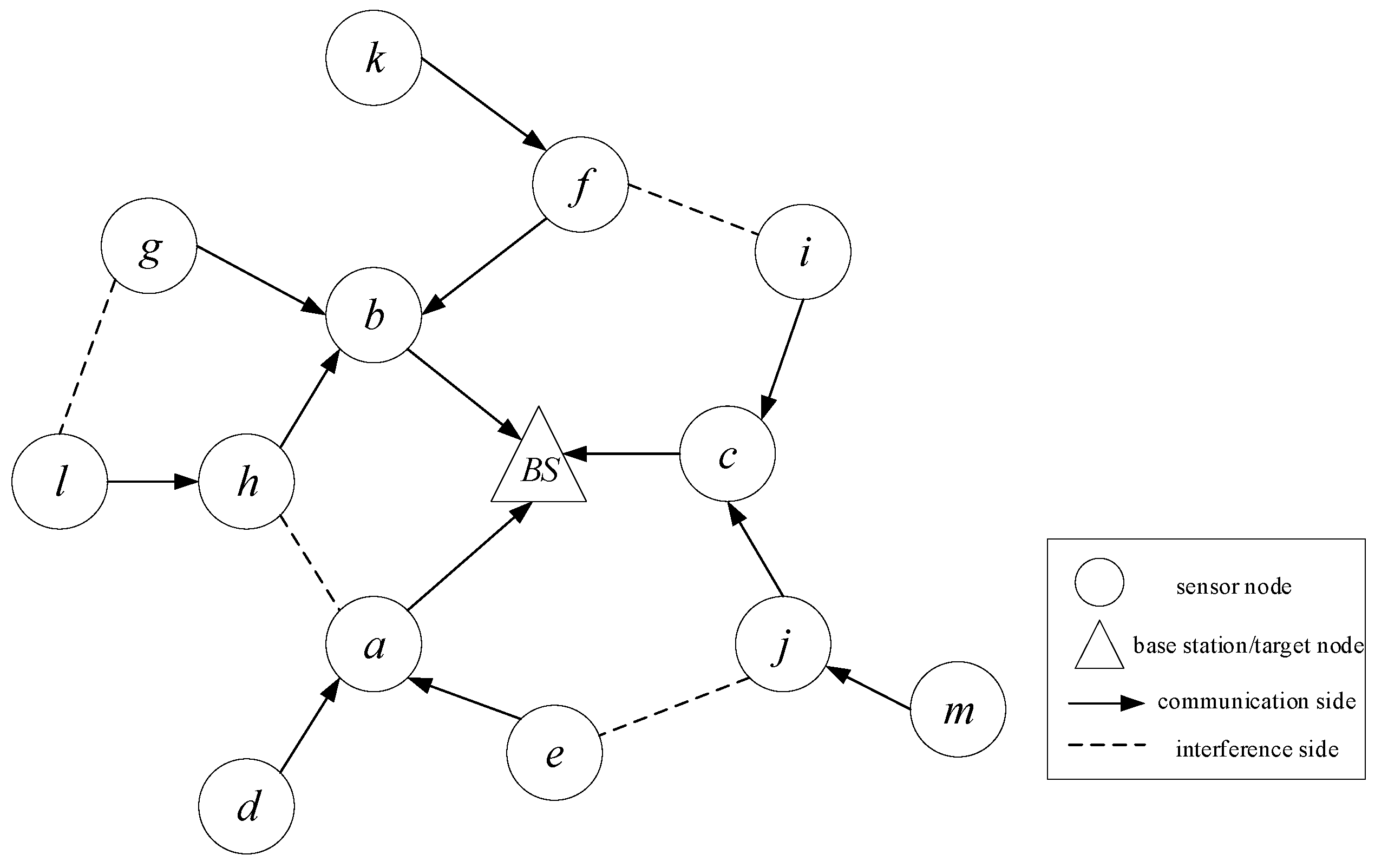
M sensor nodes and one base station node form a wireless sensor network with a known topology. As shown in Figure 1, BS is the base station or the destination node, while others are sensor nodes. The sensor nodes periodically generate data with different strict deadlines and send it to the base station node through data transmission between nodes. The entire network topology can be represented by a directed graph $G(V,E,E^{\prime })$. V represents the set of vertices of all sensor nodes. E represents the set of all communication links, $\overline{ea}$ represents node e sends data to node a, which is called the parent node of e. $E^{\prime }$ represents the set of all interference edges. Interference edge $\overline{ab}$ means that the transmission of node a will interfere with the transmission of b, and similarly, the transmission of node b will also interfere with the transmission of a.

Sensor nodes periodically generate data, and data transmission is carried out according to a time slot. The data packet $P_i$ generated by i-th node $v_i$ can be expressed as

$$P_i=(T_i,H_i,D_i,{\varphi }_i)$$

(1)

where $T_i$ is the packet generation cycle, $D_i$ is the packet transfer cutoff time, ${\varphi }_i$ is the routing path of the packet, $H_i$ represents the total hops from the source node to the sink node. The unit of $T_i$ and $D_i$ are represented by the number of time slots. Generally, $T_i$ is greater than $H_i$ to ensure the transmission time required for packets. At any time slot t, the packet contains three attributes, which are $C_i,\hspace{0.33em}{h}_i,\hspace{0.33em}{t}_i$. $C_i$ indicates the node where the data packet resides ($C_i\in {\varphi }_i$), $h_i$ indicates the number of hops remaining when data are transmitted from the current node to the destination node ($0<h_i\le H_i$), $t_i$ indicates the number of time slots contained in the remaining cutoff time of the packet ($0<t_i\le T_i$).

For the data in the process of transmission in WSNs, if the data state is $t_i>h_i$, it means that the data can be transmitted to the destination theoretically. If the next time slot is allocated by the system for data transfer, the remaining time of the current data transfer status and the remaining hops are reduced by one and the data are transmitted to the next node. Otherwise, the remaining time of the data transfer status is reduced by one. When $t_i=0$, node $v_i$ will generate new data and start to wait for transmission scheduling. The initial remaining time $t_i=T_i$ and the initial remaining hop number $h_i=H_i$.

In order to consider the practical applications, the following assumptions are assumed:

(1)

The sensor node cannot transmit and receive data at the same time or receive data from more than one node at the same time;

(2)

The node that receives multiple data selects at most one data packet for data transmission in each time slot;

(3)

The data generated periodically by the source node has a strict cut-off time limit, and the cut-off time is equal to the data generation cycle;

(4)

In the process of data transmission, if the deadline is exceeded, the data will be directly discarded because it has become invalid;

(5)

The probability of success of wireless communication transmission will be affected by physical factors such as transmission power, encoding mode, and modulation scheme. This paper assumes that if the data are arranged for transmission, the probability of success is 1.

2.2. Q-Learning Model

The data transmission scheduling in WSNs mainly solves the problem of deciding which nodes are scheduled for transmission in each time slot. The transmission status and the location of data need to be considered. The Q-learning model of WSNs data transmission scheduling problem can be represented by $(S,A,\pi ,R)$. S is the state space, representing the state set of all data in WSNs. A is the action space, representing the action set of WSNs. $\pi$ is the learning strategy of the agent, and represents the slot allocation of WSNs data transmission. R is the agent’s reward, indicating the feedback of the agent’s action in the current time slot.

(1)

System space model

The state space of the whole WSNs consists of the current state of data generated by all nodes in the network, which can be expressed as $S=\{s_1,s_2,\dots \dots ,s_{M-1},s_M\}$. The current state of data generated by any node is $s_i=\{C_i,t_i,h_i\}$. Thus, the size of the current state space of data generated by any node is $T_i{(H_i)}^2$. The size of the state space of the entire system can be expressed as ${\displaystyle \prod _{i=1}^M{T}_i{(H_i)}^2}$.

In WSNs, all possible situations of nodes conducting data transmission scheduling in each time slot constitute the action space of the system, which can be expressed as $A=\{a_1,a_2,\dots ,a_{M-1},a_M\}$. For the data generated by any node in the current time slot, if the data are transmitted, the corresponding action $a_i$ is 1; otherwise, it is 0. Regardless of WSNs sensor node transmission constraints and assumptions, the maximum movement space of the whole system is $2^M$ in theory. Thus, the size of the system can be expressed as the product of the size of the state space and the size of the action space. In such an ample system space, reinforcement learning cannot get an effective scheduling strategy. The introduction of deep reinforcement learning can be a good solution to the time slot allocation and network control problems of large-scale systems.

(2)

Value function model

The goal of reinforcement learning is to achieve mapping strategy from environment state to action $\pi :S\to A$. The Q-learning algorithm can be regarded as a random expression of value iteration algorithm. Value iteration can be expressed by action value function. $V^{\pi }(s)$ is used to represent the action value function of state s performing action a to the next state $s^{\prime }$ with probability $P(s^{\prime }|s,a)$ in the next time slot under strategy $\pi$.

$$V^{\pi }(s)=\underset{a\in A}{\max }[R(s^{\prime }|s,a)+\gamma {\displaystyle \sum _{s^{\prime }\in s}P(s^{\prime }|s,a)V^{\pi }(s^{\prime })}]$$

(2)

where $P(s^{\prime }|s,a)$ represents the transition probability that the system performs action a in state s and turns to state $s^{\prime }$. $R(s^{\prime }|s,a)$ represents the average reward for state transitions. $\gamma$ is the discount factor, $\gamma \in (0,1)$, which reflects the impact of future income on the current state. The optimal strategy is to obtain the execution action that maximizes the value function. The optimal strategy ${\pi }^{\ast }(s)$ can be expressed as follows:

$${\pi }^{\ast }(s)=\arg V^{\ast (\pi )}(s)=\underset{a\in A}{\arg \max }[R(s^{\prime }|s,a)+\gamma {\displaystyle \sum _{s^{\prime }\in S}P(s^{\prime }|s,a)V^{\pi }(s^{\prime })}]$$

(3)

In the Q-learning model, the Q value update of the system is defined as follows:

$$Q_t(s_t,a)=(1-\partial )Q_t(s_t,a)+\partial [R(s^{\prime }|s,a)+\gamma {\displaystyle \sum _{s^{\prime }\in \in S}P(s^{\prime }|s,a)\underset{a\in A}{\max }{Q}_t(s^{\prime }|s,a)}]$$

(4)

where $\partial \in (0,1)$ is the learning rate factor. The larger $\partial$ is, the more the system learning process depends on the reward function and the value function. The smaller $\partial$ is, the more the system relies on the accumulated learning experience, and the slower the learning rate. The Q-learning algorithm maximizes the system utility by calculating and updating the Q value, but $P(s^{\prime }|s,a)$ is usually unknown, and in the Q-learning algorithm, $R(s,a)+{\displaystyle \sum _{s^{\prime }\in s}P(s^{\prime }|s,a)\underset{a\in A}{\max }}{Q}_t(s^{\prime }|s,a)$ can be directly replaced by an unbiased estimate constructed from the current transformation $R_{t+1}+\underset{f\in A}{\max }Q(s_{t+1},a_t)$, so as to obtain the final Q The value function updates the formula as:

$$Q_t(s_t,a)\leftarrow (1-\partial )Q_t(s_t,a)+\partial [R(s^{\prime }|s,a)+\gamma \underset{a\in A}{\max }{Q}_t(s^{\prime }|s,a)]$$

(5)

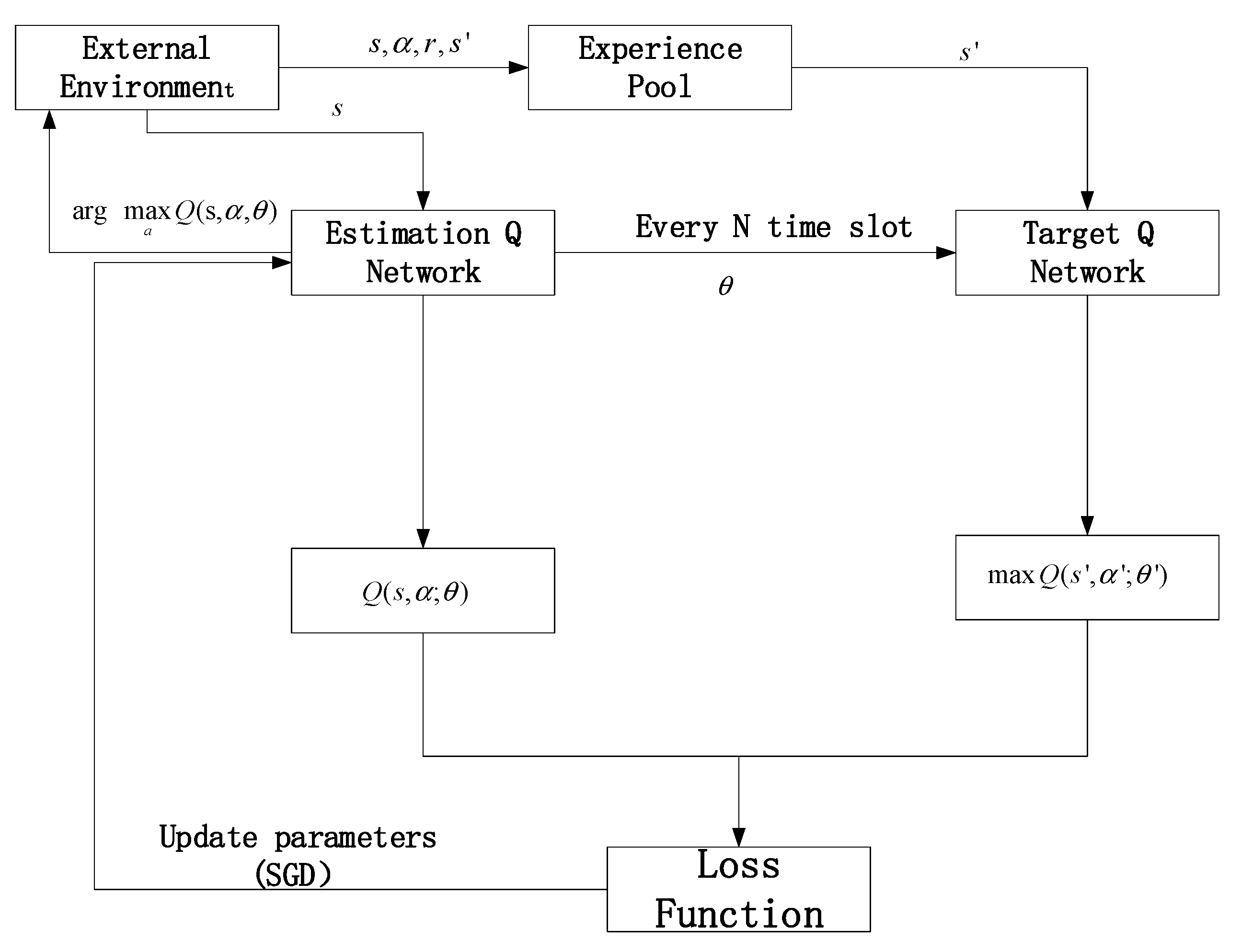
2.3. DQN Network Model

The role of the neural network in the DQN network model is to realize the supervised learning of WSNs. The general method constructs two Q networks, in which the experience pool provides training samples, the loss function is determined by the target Q value and the calculated Q value, and then the gradient is calculated, using the stochastic gradient descent method (SGD) updates the parameter W and the bias b. The DQN network model is shown in Figure 2.

Two networks with the same structure but different parameters are established in Figure 2 [24]. One network uses the latest parameters to calculate and predict the Q value, and the other network uses the parameters before a certain time to update the Q value. This can ensure the stability of the target Q value for a period of time, reduce the correlation between the current Q value and the target Q value to a certain extent, and make the performance of the algorithm more stable.

The experience pool is also known as experience replay. Its role is not only to solve the problem of data correlation but also to provide learning samples. A memory bank is established at the beginning of the learning and training process. The state, action, reward, and the state of the next time slot after executing the current action are stored in the experience pool. Each time a neural network is trained, a certain amount of memory data is randomly sampled in batches from the experience pool. At the same time, when the experience pool is full, the new memory will overwrite the old memory, thus disrupting the order of the original data and further weakening the relevance of the data.

3. Proposed Algorithm

In this section, the algorithm is divided into three parts: optimal action selection strategy, reward mechanism, and state-behavior description network. We describe the above three parts in Section 3.1, Section 3.2 and Section 3.3, respectively. Finally, the overall flow of the algorithm is given in Section 3.4.

3.1. Optimal Action Selection Strategy

The optimal action selection strategy is used to determine the node-set to send. Firstly, the strategy selects the best action for the current time slot by exploring the development strategy. Secondly, based on the node where the action is located, the most urgent and non-conflicting node-set is constructed.

(1)

Explore development strategies

In the process of systematic learning and trial and error, it is necessary to balance the relationship between exploration and development. The general $\epsilon -greddy$ strategy is prone to the problem of too fast convergence. Development under the condition of insufficient exploration will cause the learning process to be too short and the learning results to be seriously deviated. Based on the $\epsilon -greddy$ strategy, this algorithm introduces the Metropolis criterion in the simulated annealing algorithm into the execution action selection of the exploration and development strategy. Meanwhile, it can be seen from the Q learning model that the state space of the whole system explosively expands with the increase of the number of nodes, which requires relatively long learning times to achieve the ideal training effect. Therefore, segmented exploration and development processes are adopted to acquire state and behavior. In the early stages of DQN network learning, actions are randomly selected and saved to the experience pool before the experience pool is full. Then, based on the exploration probability ${\epsilon }_t$, the action selection begins to gradually balance the exploration and development process, which can better solve the problem of too fast convergence. The exploration probability ${\epsilon }_t$ is defined as follows:

$${\epsilon }_p=\exp [\frac{-|\underset{a_0\in A}{\max }a\_value(s,a_0)|}{K{T}_k}]$$

(6)

$${\epsilon }_t=\max \{{\epsilon }_{\min },{\epsilon }_p\}$$

(7)

${\epsilon }_p$ is the exploration probability after the simulated annealing algorithm is introduced, where $\max a\_value(s,a_0)$ is the maximum output value after the state-action mapping in the deep neural network, and $a_0$ is the action corresponding to the maximum output. $T$ is a fixed value, $K$ is a coefficient, satisfying $K={\lambda }^e$, $\lambda \in (0,1)$. e is the number of learning times. As the number of learning times increases, the value of $K{T}_k$ will become smaller and smaller, and the value of ${\epsilon }_p$ will also become smaller and smaller, and the entire exploration process will tend to be stable. ${\epsilon }_{\min }$ is the given minimum exploration probability, which is the lower bound of exploration, ${\epsilon }_t$ is the final exploration probability of the current time slot, and it is the maximum value of ${\epsilon }_p$ and ${\epsilon }_{\min }$. When the best action is selected, to utilize the network’s transmission capacity as much as possible, other nodes are selected for concurrent transmission. The process is mainly based on the conflict interference matrix and the urgency of the data.

(2)

Concurrent node sets based on the most urgent data

Although each time slot allows multiple nodes to transmit data, there are transmission conflicts between child nodes with the same parent node, and two sensor nodes with interference edges cannot perform transmission tasks simultaneously. In this algorithm, the deep neural network mapping relation is used to determine the most urgent data, and the node where the data resides is the most urgent node. Then, other transmission nodes are dynamically selected to construct the most urgent non-conflicting node-set and transmit the selected data from the node.

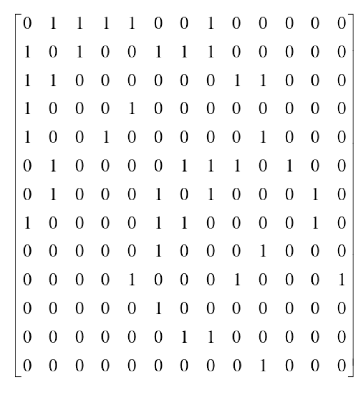
Definition 1.

A conflict interference matrix is used to represent the matrix of the conflicted relationship between nodes, where the row number and column number respectively represent the number of the corresponding sensor node. If there is conflict or interference between nodes, the corresponding matrix element is represented by 1; otherwise, it is represented by 0.

The conflict interference matrix MC is constructed based on the WSNs topology, as shown in Figure 3 is the conflict interference matrix based on Figure 1.

Definition 2.

Data urgency indicates the urgency of data to be sent in a certain time slot, represented by u_i. It is related to the number of remaining hops h_i and the remaining deadline t_i. The data urgency can be expressed as follows:

$$u_i=h_i/(t_i\ast (t_i-h_i))$$

(8)

The steps to determine the concurrent node set are as follows:

Step 1: Construct the conflict interference matrix, determine the most urgent node N by the best action, and add this node to the concurrent node-set;

Step 2: Add the node (excluding node N) with column coordinates corresponding to the value of 0 in the n-th row of matrix MC to the list to be transmitted;

Step 3: Calculate the urgency of other data on the network. If the node with the highest urgency is in the list to be transmitted, add the node to the concurrent node-set. Then, remove the node from the list to transfer. If the data are not in the list to be transmitted, ignore the data and repeat Step 3.

Step 4: If the list to be transmitted is not empty, continue step 3 until the list to be transmitted is empty and obtain the final concurrent node-set based on the most urgent data.

Taking Figure 1 and Figure 3 as an example, assuming the current time slot, the data $data\_g$ generated by node g are selected as the most urgent data through the exploration and development strategy, and the node where the data $data\_g$ are currently located is b. In step 1, it is determined that node b is added to the concurrent node-set. In step 2 and the conflict interference matrix, nodes d, e, i, j, k, l, and m are added to the list to be transmitted. In step 3, calculate the data state urgency evaluation ct generated by other nodes except the data generated by node g, select the data with the highest evaluation value and the node where the data are currently located in the transmission list, and add the node to the concurrent node-set. Assuming that the node is j, update the transmission queue and remove nodes e, i, j, and m. Continue to select the node with the most urgent data in the list to be transmitted to join the concurrent node-set and update the list to be transmitted. Repeat step 3 until the list to be transmitted is empty, then the final of concurrent node-set $\{b,d,j,k,l\}$ can be obtained.

3.2. Reward Mechanism

The establishment of the reward function in this section considers two factors: the immediate reward of real-time data allocated to the time slot and the influence of other data not allocated to the time slot. Instant reward r reflects the current priority of the data by considering the remaining time of the node and the number of hops remaining for all the data allocated by the time slot. The function $R_L$ is defined to represent the impact of other data flows that are not allocated to time slots at the current time. When the current time slots are allocated, the more packets of other data flows are lost, the closer the data distance to the discarded state is, and the greater $R_L$ is. The reward function is shown as

$$R=r+R_L$$

(9)

where r represents the instant reward value of all packets allocated to time slots. The instant reward value of each data packet allocated to time slots consists of the remaining time of the packet and the remaining hops. The smaller the remaining time is, the longer the remaining hops are, and the larger the r is, the higher the priority of the current packet is. Immediate rewards are defined as follows:

$$r={\displaystyle \sum _{i=1}^n{\beta }_i\cdot (k_1}\cdot \frac{h_i}{t_i}+k_2\cdot \frac{1}{t_i-h_i+1})$$

(10)

where $t_i\ge h_i$, and n represents the number of packets to obtain slot assignments. If data i are transmitted in the current time slot and arrives at the destination node, the reward is enhanced, ${\beta }_i\in [1,1.5)$, otherwise ${\beta }_i=1$. $k_1,k_2$ satisfies $k_1>0,k_2<1$, and $k_1+k_2=1$. Obviously, r is inversely proportional to the remaining packet cutoff time $t_i$ and is directly proportional to the remaining hop number $h_i$ of the packet. Both $h_i/t_i$ and $t_i-h_i$ can reflect the degree of urgency of data. $h_i/t_i$ reflects the degree of urgency of data through ratio relationship without considering the influence of actual remaining time slots. $t_i-h_i$ reflects the influence of actual remaining time slots.

$R_L$ is the reward function of behavior, which reflects the negative reward. When the system is in state $s_i$ and performs an action to enter the next state $s_{i+1}$, it is assumed that among all data packets in the system, $L_{i0}$ data packets meet the transmission state of $t_i-h_i=-1$, $L_{i1}$ data packets meet the transmission state of $t_i-h_i=0$, and $L_{i2}$ data packets meet the transmission state of $t_i-h_i=1$.

$$R_L=-({\rho }_1{L}_{i0}+{\rho }_2{L}_{i1}+{\rho }_3{L}_{i2})$$

(11)

where $L_{i0}$, $L_{i1}$, and $L_{i2}$ are defined as above, ${\rho }_1$, ${\rho }_2$, and ${\rho }_3$ are relevant discount parameters, satisfying $0<{\rho }_1,{\rho }_2,{\rho }_3<1$, ${\rho }_1>{\rho }_2>{\rho }_3$, and ${\rho }_1+{\rho }_2+{\rho }_3=1$. The final reward function is expressed as follows:

$$R={\displaystyle \sum _{i=1}^n{\beta }_i\cdot (k_1\cdot \frac{h_i}{t_i}+k_2}\cdot \frac{1}{t_i-h_i+1})-({\rho }_1{L}_{i0}+{\rho }_2{L}_{i1}+{\rho }_3{L}_{i2})$$

(12)

The partial separation and combination of reward parameters and reward factors allow the reward function to adjust the external weight. The behavior of the whole system is determined by the initial state of the data flow and the reward function of the behavior. The system can converge to the ideal equilibrium point in a given environment.

3.3. State-Behavior Description Network

The deep neural network is a kind of neural network containing multiple hidden layers, each of which can perform the nonlinear transformation on the output of the previous layer. Therefore, compared with a shallow layer network, a deep neural network has more excellent expression ability and can learn more complex function relations in a more compact and concise way.

The Stacked Auto Encoder (SAE) deep neural network consists of multiple layers of sparse autoencoder neural networks. The general idea of the training process is unsupervised pre-training and supervised fine-tuning. In this network, in the unsupervised training stage, the hidden feature representation learned by the previous layer of autoencoders is used as the input of the latter layer of autoencoders. The training process of the parameters of each layer will keep the parameters of other layers fixed. After the above-mentioned pre-training process is completed, in the supervised fine-tuning stage, using the previously trained parameters as the initial value of the network, the parameters can also be adjusted, and then continue to train the neural network.

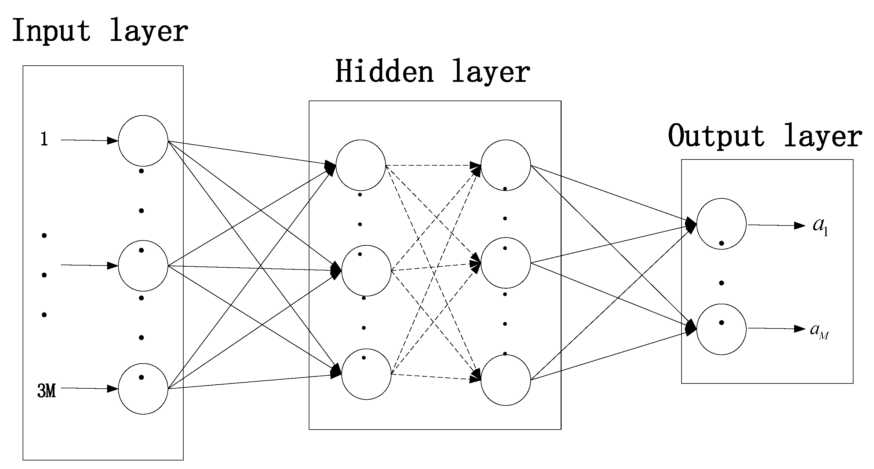
This algorithm adopts the multi-layer stacked self-encoding deep neural network model to train and realize the mapping relationship between the system state and behavior, which can quickly obtain the optimal decision-making behavior. The structure of the SAE model is shown in Figure 4. The input layer of the model corresponds to the state information of the system, and the number of neurons in the input layer is $3\cdot M$. The input vector is composed of the current transmission state of the data generated by all nodes of the WSNs, including the node where the data are currently located, the remaining hops, and the remaining deadline. All input vectors are denoted as $input=[c_1\dots c_M{h}_1\dots h_M{t}_1\dots t_M]$. The output layer represents the action selection information of the model, and each output corresponds to each node to generate data in the system as the evaluation of the most urgent data in the next time slot, so the number of neurons in the output layer is M. The output vector is $output=[a_1\dots a_M]$. The hidden layer is multi-layered, and the number of neurons in each layer is related to the number of sensor nodes in the network.

The neurons of the hidden layer in the SAE model are activation functions used for the nonlinear transformation of the input information. Common activation functions include ReLU function, sigmoid function, and tanh function. The nonlinear sigmoid function has a large signal gain in the central area and relatively small signal gain on both sides, which has a good effect on the feature space mapping of the signal. The activation function of this algorithm selects the sigmoid function. The loss function of the overall sample during the training process is denoted as $L(W,b)$.

$$L(W,b)=\frac{1}{N}{\displaystyle \sum _{i=1}^{N}l(W,b)}$$

(13)

where $N$ is the total number of input samples, $l(W,b)$ is the loss function of a single sample, and the calculation expression of $l(W,b)$ is as follows:

$$l(W,b)=\left\{\begin{array}{c}\frac{1}{2}{(q_{eval}-q_{tgt})}^2,|q_{eval}-q_{tgt}|\le 1\hspace{0.33em}\hspace{0.33em}\\ |q_{eval}-q_{tgt}|-\frac{1}{2},\hspace{0.33em}\hspace{0.33em}\hspace{0.33em}\hspace{0.33em}\hspace{0.33em}\hspace{0.33em}otherwise\end{array}\right.$$

(14)

where $q_{eval}$ represents the calculated Q value, and $q_{tgt}$ represents the target Q value. When the forward propagation process is over, the parameter W and the bias b are updated using the gradient descent method.

3.4. Proposed Algorithm Description

The proposed real-time data transmission scheduling algorithm based on deep Q-learning (RS-DQL) comprehensively considers the influences of communication constraints and interference between sensor nodes in WSNs, the remaining cutoff time, and the variation of the remaining hop count in the process of data transmission and scheduling. It uses deep neural networks to evaluate state-action mapping relationships and is updated by Q-learning methods. In addition, the empirical replay was introduced to reduce data relevance and adapt to the randomness of the training process.

The idea of RS-DQL algorithm is as follows: Firstly, the data transmission and communication interference model of WSNs is constructed to determine the concurrent node-set based on the most urgent data. The Q-learning algorithm is used to acquire partial state transfer information (including the current state, the action to be performed, the reward to be obtained, and the next state) and store it into the experience pool after a certain time slot. This process does not train the SAE network model. After a period of time, samples are extracted from the experience pool and combined with the DQN network model for supervised training of the SAE network. In the process of network model learning and training, the system gradually rewards the actions with less packet loss for data transmission to achieve an approximate optimal scheduling algorithm.

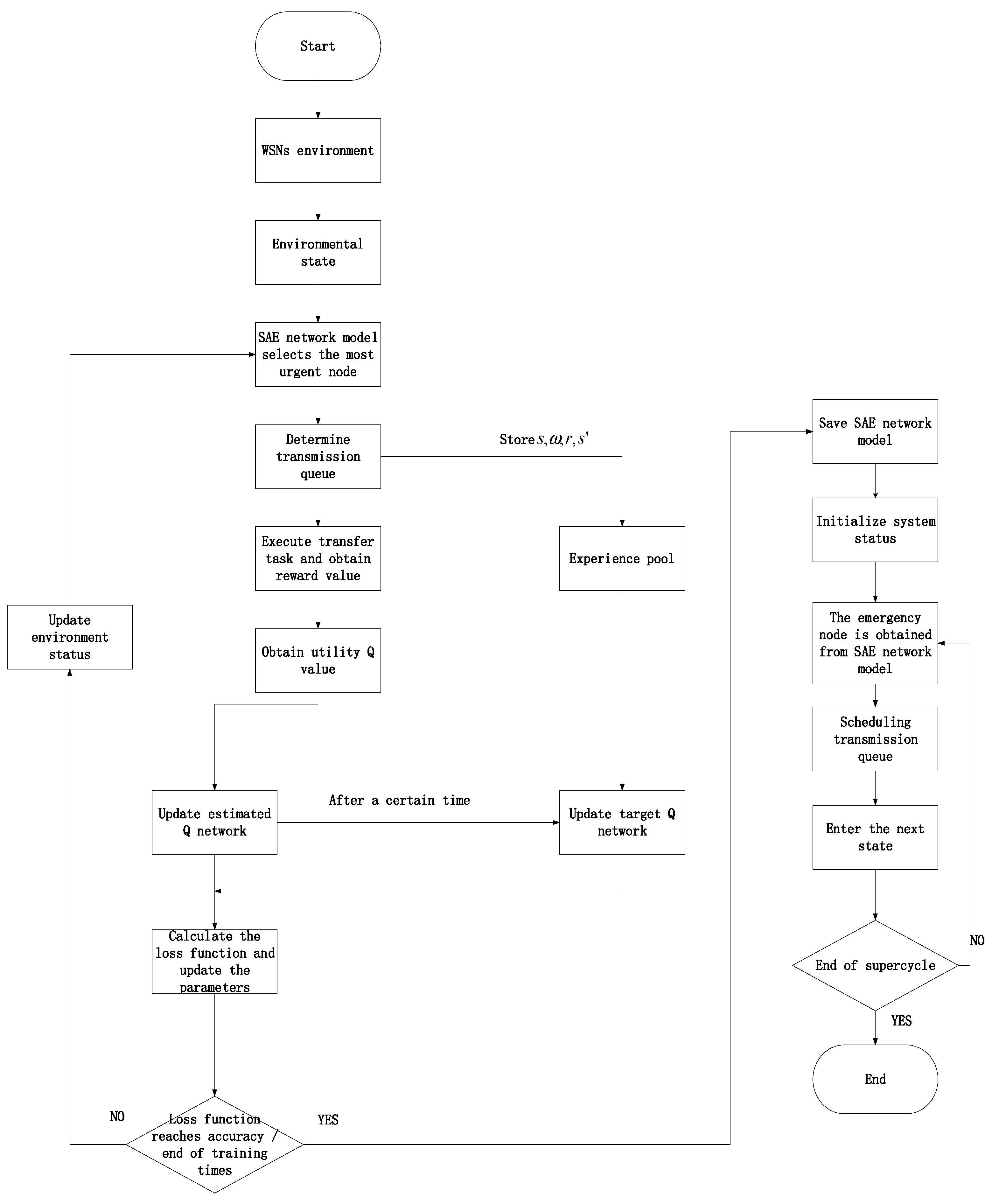
The scheduling algorithm flow of RS-DQL is shown in Figure 5. Firstly, before the experience pool is full, the SAE network model randomly selects actions. The Q-learning algorithm learns a part of the state and action data based on the selected actions. After the experience pool is full, the SAE network is gradually trained. Its parameters are updated with supervision during the learning process. When the system shifts to the hidden state, the SAE network recommends the system’s actions in this state, performs the actions, updates the Q value network, etc. Repeat the learning process until the loss function reaches the target accuracy or the expected number of training sessions. Finally, the data transmission scheduling of the system is carried out by the state-action mapping in the trained SAE network model.

The process description of the real-time data transmission scheduling algorithm based on deep Q-learning can be obtained from the above system model and scheduling strategy. However, this algorithm studies the scheduling problem of multiple concurrent data transmission in WSNs. How to allocate data transmission tasks in each time slot is related to behavior acquisition and training effect in the process of deep Q-learning. According to the exploration and development strategy, the most urgent data are first determined as the current time slot execution action a. Based on the most urgent data and system status, multiple data that can execute the transmission task simultaneously in the current time slot are determined. Add a to the waiting queue, and then select the data that do not conflict with all data transmission in the waiting queue according to the degree of urgency. The data that do not conflict with other data transmission in the waiting queue are selected repeatedly until the maximum amount of data transmission is reached. The state process of system state information is guided by action strategy. SAE network model establishes the mapping relationship between states and actions. Finally, the DQN network model is used for training to obtain the final node scheduling strategy. The specific algorithm description is shown in Algorithm 1.

Algorithm 1 RS-DQL algorithm

1: Randomly initialize the parameters, import the WSNs environment, $episod{e}_1=1$ 2: for episode = 1 to M do 3:    Initialize the current state s, time slot number T, $episod{e}_2=1$ 4:    while $episod{e}_2<T$, do

5:       Action $a$ is determined according to the exploration and development strategy, and it is added to the transmission waiting queue L 6:       Add the remaining theoretically reachable data $(t\ge h$$)$ without conflicting data transmissions, $w=100,\hspace{0.33em}{a}_1=-1$ 7:       if $L^{\prime }$ is not empty do 8:         Take data $i$ in turn from $L^{\prime }$ and calculates $h_i/(t_i\cdot (t_i-h_i))$ 9:         if $h_i/(t_i\cdot (t_i-h_i))<w$$\mathrm{and} t_i\ge h_i$, do 10:          $a_1=i,\hspace{0.33em}w=h_i/(t_i\cdot (t_i-h_i))$ 11:        else return to step 7 12:      end if 13:        if $a_1>0$ do 14:           Add  $a_1$ to queue L, and return to Step 6 15:        else Determine the transmission queue L 16:        end if 17:       Perform the action a, calculate the reward R, and move to the next state $s^{\prime }$ 18:      Put $(s,a,r,s^{\prime })$ into the experience pool 19:      if The experience pool is full do 20:        Enter the learning process and calculate $q_{eval},\hspace{0.33em}{q}_{tgt},\hspace{0.33em}loss$ 21:        if Current loss is minimum do 22:            Update loss and store the network parameter model 23:        end if 24:        $s=s^{\prime },\hspace{0.33em}episod{e}_2+=1$ 25:      end if 26:    end while 27:    if Loss meets the accuracy requirements do 28:      break 29:    end if 30:    $episod{e}_1+=1$ 31: end for 32: The training is completed and the final SAE network parameter model is obtained

33: The node scheduling strategy was obtained by importing WSNs environment and SAE network parameter model

4. Simulation Results

The simulation experiment considers the network performance of WSNs data packets with different random deadlines for transmission scheduling. The objective is to minimize the number of lost packets (that is, the number of packets that are discarded when the remaining deadline is less than the remaining hop count during data transmission). In the simulation experiment, a long time slot is taken to analyze and compare the number of lost packets in this time slot for convenient comparison. Other parameters of the simulation are shown in

Table 2. Simulation parameters.

Parameters	Value
Learning Rate	$\partial =0.01$
Discount Factor	$\gamma =0.9$
Instant Reward r	$k_1=k_2=0.5$
	${\beta }_i=1$
Delay Reward RL	${\rho }_1=0.5,{\rho }_2=0.3,{\rho }_3=0.2$
	${\epsilon }_{\min }=0.01$
Correlation Coefficient of Development Strategy	$\lambda =0.98$ $T_k=1000$
Episode	400
Number of Neurons in Each Layer of SAE	$[3M,26,26,13,M]$
Nodes Count	13
Nodes Topology	Presented in Figure 1
Matrix of Interference between Nodes	Presented in Figure 3
Packet Cutoff Time	Randomly generated for each packet

.

The real-time data transmission scheduling algorithm based on deep Q-learning is named the RS-DQL algorithm. There are two algorithms for comparison, including the classical EDF algorithm and an enhanced dynamic multi-priority data scheduling algorithm (EDP algorithm) [25]. The idea of the EDF algorithm is the earliest deadline first. The transmission queue of each time slot system is composed of multiple non-conflicting nodes with the shortest deadline. The idea of the EDP algorithm is to divide priority queues for data characteristics in the system, such as emergency data and periodic data. In the same queue, the priority of data transmission is determined according to the relationship between the remaining time of the current transmission state of different data and the remaining hop number. This chapter analyzes the network performance comparison between the RS-DQL algorithm and the other two algorithms under different conditions such as data deadline and the number of network nodes.

In

Table 3. Average number of lost packets for different algorithms.

Algorithm	EDF	EDP	RS-DQL
Number of lost packets	1569	1227	935
Number of successfully sent packets	1665	2007	2299
Packet loss rate	48.52%	37.94%	28.91%

, the network topology of the simulation experiment is based on the communication interference diagram of WSNs sensor nodes in Figure 1. The data generation cycle of each sensor node is randomly set as 1.5 to 3.5 times the total hop number of sensor nodes. Therefore, small multiples represent short packet cutoff time, and large multiples represent long packet cutoff time. As shown in the table, the performance of the RS-DQL algorithm is significantly better than the other two algorithms, followed by the EDP algorithm. The scheduling performance of the EDF algorithm is nearly half of that of the RS-DQL algorithm, and it is the worst among the feasible algorithms.

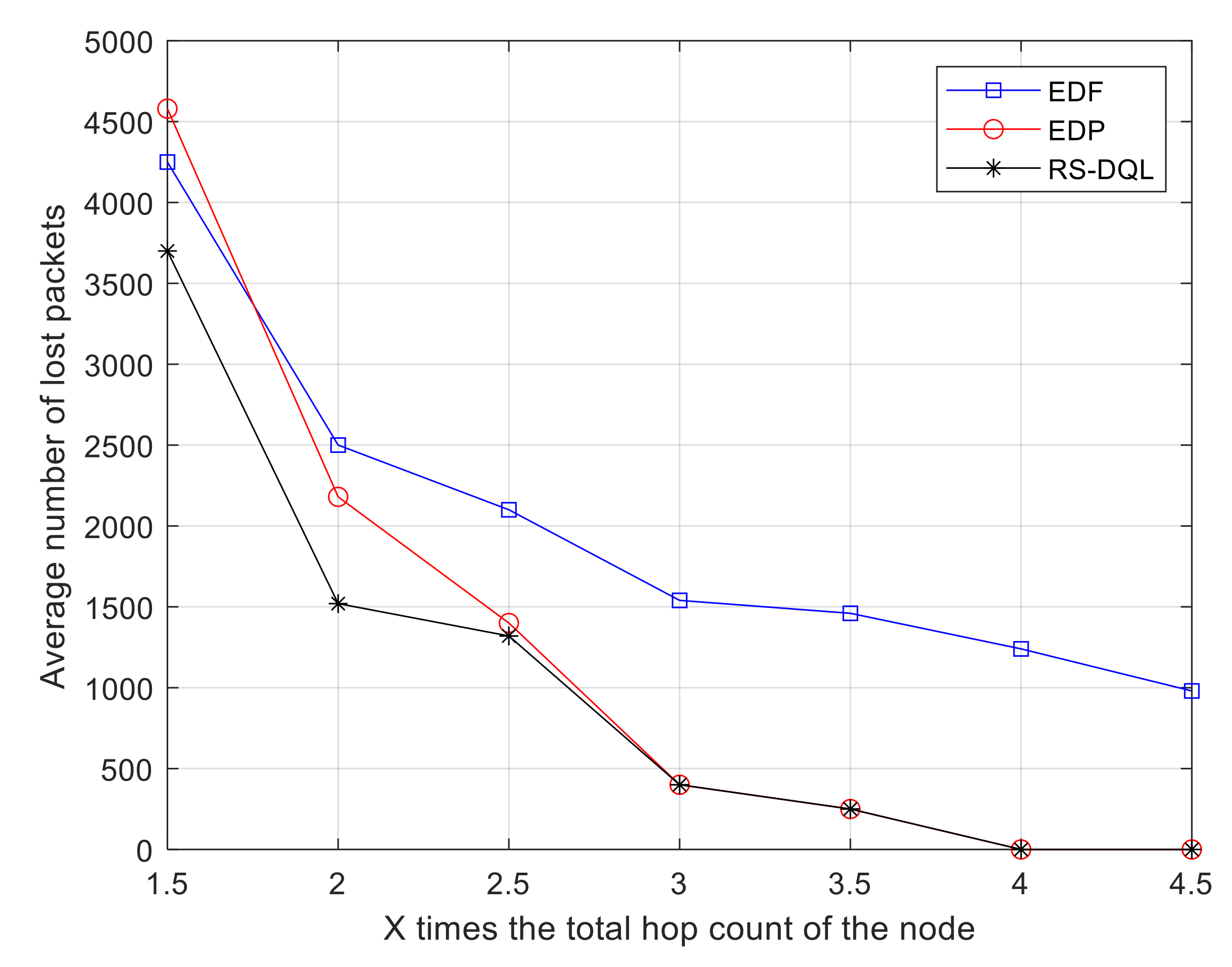
Figure 6 considers the changes in packet loss of the three algorithms as the size of the data generation cycle of the sensor node is an integer multiple of the total hop number of the node. In WSNs, the generation period of sensor node data is increased by 1.5 to 4.5 times the total hop count of the node. As the data generation period lengthens, the packet loss of the three algorithms decreases. The performance of the EDP algorithm is poor before 2.5 times, and is basically the same as the RS-DQL algorithm after 2.5 times. When the multiple is 4, the number of packets lost by EDP and RS-DQL is 0. However, the RS-DQL algorithm has the best performance and is more stable in the whole process. EDP algorithm has the largest variation with the increase in the data generation cycle. In contrast, the EDF algorithm has the lowest overall performance.

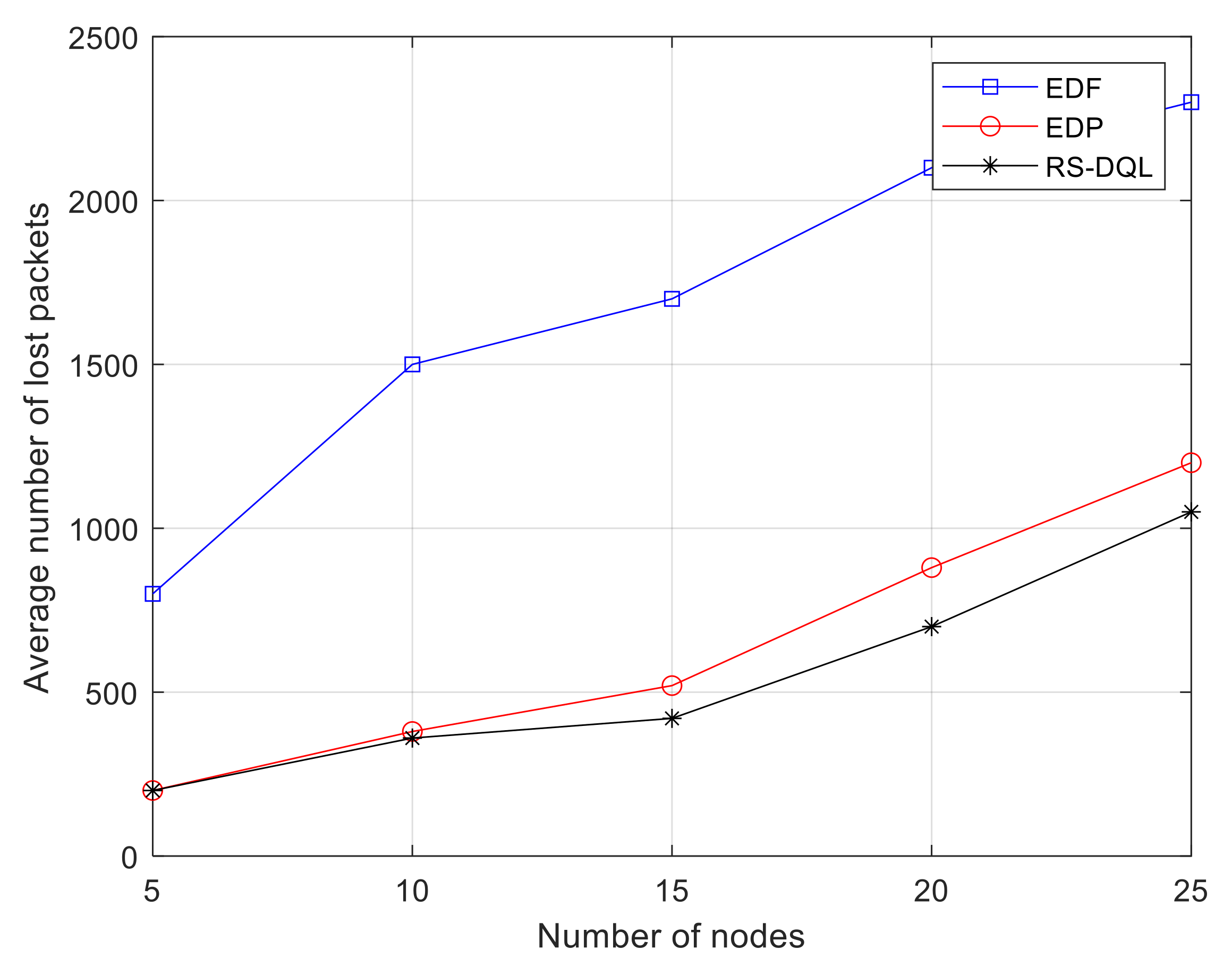
Figure 7 considers the changes of packet loss of the three algorithms as the number of sensor nodes increases from 5 to 25 in the case that the data generation cycle in WSNs is 3 times the total hop number between sensor nodes and destination nodes. As the number of nodes increases, the performance of the EDP algorithm is similar to the RS-DQL algorithm. Although the EDP algorithm has a good advantage when the data generation cycle of sensor nodes is a large integer multiple of the total hop number of data transmission, such as 3 times or more, the RS-DQL algorithm is still superior to EDP algorithm in overall network performance. The number of loss packets of the EDF algorithm is always high. When the data generation cycle is an integer multiple of the total hop number, the disadvantage of the EDF algorithm will be magnified. Therefore, the EDP and RS-DQL algorithms are better than the EDF algorithm.

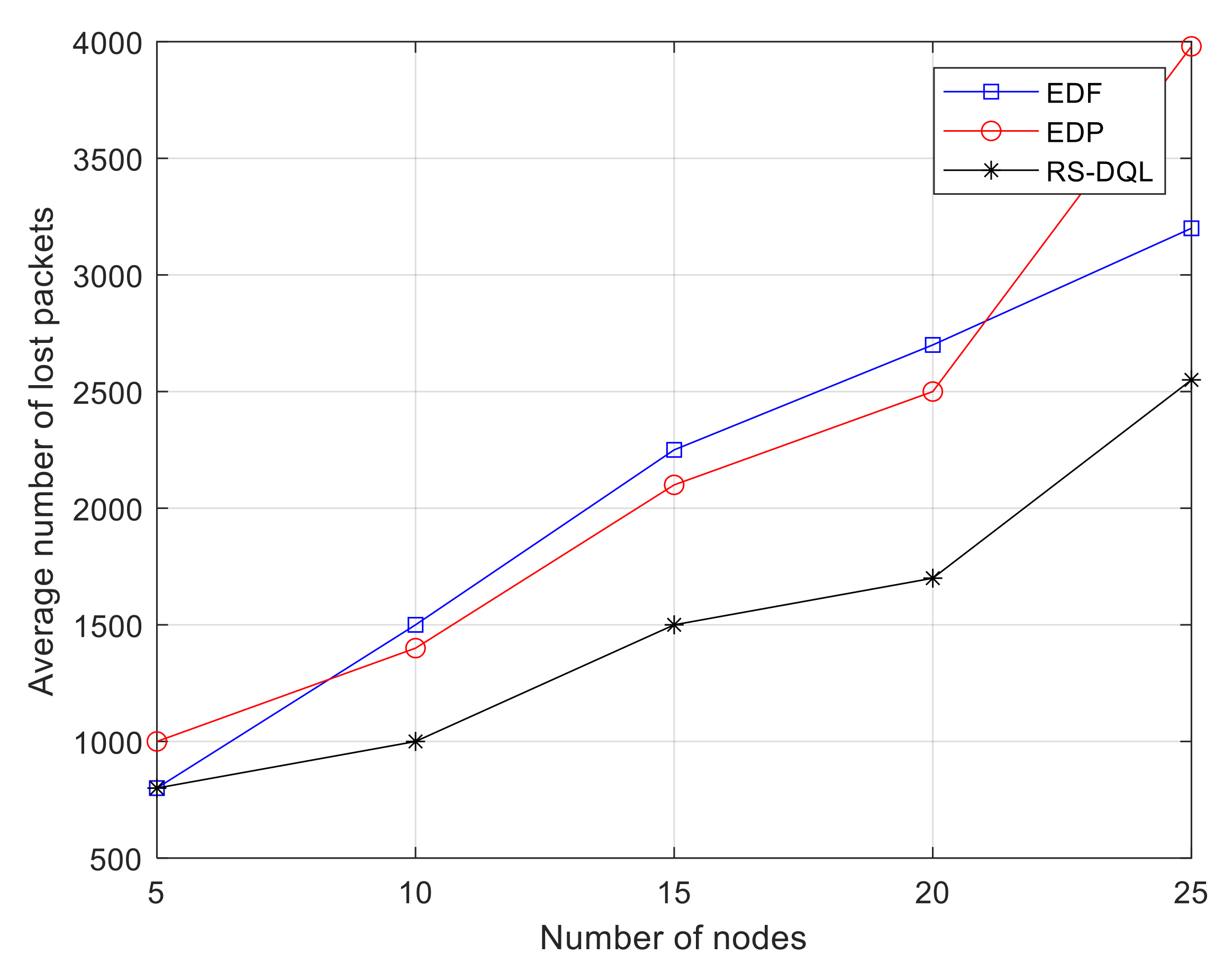
Figure 8 considers the changes of packet loss of the three algorithms in WSNs as the number of nodes gradually increases from 5 to 25. At this point, the generation period of sensor node data is a random value between 1.5 times and 3.5 times the total node hops. As the number of nodes increases, the number of lost packets of the EDF algorithm changes almost linearly. However, the EDP algorithm is not stable. With the increase of sensor nodes to 20, the increase of packet loss of this algorithm is significantly more than the other two algorithms. This indicates that the algorithm has inferior performance in WSNs with a large number of nodes and random deadlines. The RS-DQL algorithm is stable, and the number of lost packets is always the smallest, and the increase rate of lost packets is relatively stable.

It is worth noting that although the simulation results in this paper are based on the topology in Figure 1, the strategies proposed in this paper are also applicable to other structures. When the topology structure of the network changes, the conflict interference matrix of Figure 3 needs to be calculated according to the topology structure. Then, the network is retrained according to the process in Section 3.4, and the algorithm proposed in this paper can be used in the new topology after the training is completed.

The RS-DQL algorithm proposed in this paper obtains the most urgent data through the state-behavior description relationship of neural network in its Q-learning part. According to the network topology and data urgency, the concurrent node set based on the most urgent data is determined, so as to obtain the optimal action selection strategy. In the reward function formulation part, the goal is to transmit as much data as possible in WSNs to the destination node within its deadline. Consider the influence of factors such as communication constraints between nodes, data remaining deadline and remaining hops, and give reward and punishment feedback after the agent performs the action. In the deep learning part, a DQN network model is built. The SAE network model is used to establish the mapping relationship between state and behavior. The data transmission slot scheduling strategy of sensor nodes is obtained through DQN network model training.

5. Conclusions

This paper mainly studies the data transmission scheduling strategy in WSNs. It proposes a real-time data transmission scheduling algorithm for WSNs based on deep Q-learning in the case of parallel data transmission in wireless sensor networks. The proposed algorithm solves the data transmission scheduling problem of WSNs with strict deadlines and minimizes the number of lost packets. The deep Q-learning method is introduced into the field of WSNs, and its network performance is improved and optimized.

However, there are still problems to be studied in the future. The construction and training of deep learning model is very critical and challenging. Although the SAE network model built in this paper can improve the network performance of WSNs after training, the DQN network model used is relatively simple. In the follow-up research, we can consider optimizing the DQN network model, and there is more research work for the setting of relevant parameters. In addition, the simulation experiment part of this paper was realized by simulation on the computer side. It uses a relatively ideal network environment, which deviates from the characteristics of the actual application scenario. In the future, hardware equipment can be used to further improve the simulation part.