A Novel Approach for the Implementation of Fast Frequency Control in Low-Inertia Power Systems Based on Local Measurements and Provision Costs

Abstract

Transitioning towards carbon-free energy has brought severe difficulties related to reduced inertia in electric power systems. Regarding frequency stability, low-inertia systems are more sensitive to disturbance, and traditional frequency control is becoming insufficient to maintain frequency within acceptable limits. Consequently, there is a necessity for faster frequency support that can be activated before the primary frequency control and that can decelerate further frequency decay. This paper proposes a local control strategy for a multi-stage fast frequency response (FFR) provided as an ancillary service that considers the location of the disturbance and the distribution of system inertia. The novelty of the presented control strategy is the ranking of FFR resources by price, which takes the economic component into consideration. The proposed control is simple, based only on RoCoF measurements that trigger the activation of FFR resources. Its advantage over other methods is the ability to adapt the FFR resource response to the disturbance without complex calculations and the ability to ensure a bigger response closer to the disturbance, as well as in low-inertia parts of the system. In that way, there is a bigger activation of resources in the parts of the system that are more endangered by disturbances, which, as a result, minimizes the propagation of the disturbance’s impact on system stability. The applicability of the presented method is demonstrated in a simple 3-area power system and IEEE 68-bus system implemented in MATLAB/Simulink. The results show that the proposed control enables the largest response closer to the disturbance, thus mitigating the propagation of the disturbance. Furthermore, the results confirm that the proposed control enables lower provision costs and more support in low-inertia areas that are more vulnerable to disturbances.

1. Introduction

The increasing integration of converter-connected renewables, along with phasing out of coal-fired power plants, contributes to a decrease in power system inertia. Reduced inertia diminishes the ability of an electric power system (EPS) to withstand frequency deviations after a disturbance [1,2]. As a result, large frequency deviations and, consequently, high values of the Rate of Change of Frequency (RoCoF) can cause cascading outages that can lead to a system blackout [1]. Additionally, frequency deviations are not simultaneous and equally distributed across the EPS [3]. Therefore, a large disturbance can potentially trigger the islanding of part of a system, especially in the case of a non-uniformly distributed inertia [4]. Large and fast changes in frequency after a disturbance are particularly common in naturally isolated power systems that have a high share of solar and wind farms, such as Ireland [5], the United Kingdom [6] and South Australia [7]. Problems of this kind are expected to become even more critical with current decarbonization ambitions [8]. The conventional primary frequency control (PFC), provided by synchronous generators, is no longer fast enough to reliably limit frequency deviations in low-inertia systems [9,10,11,12,13]. For this reason, it is necessary to consider new solutions for frequency control that can be adapted to the power system with a large share of power electronics devices, and this was the initial incentive for our paper.

Some solutions suggest limiting the share of non-synchronous generation, i.e., the constraint that refers to the minimum required inertia [9], or reducing the size of the largest generation unit [11] to ensure stable power system operation. Although these applications can keep the frequency within the allowed limits, they are not cost-effective or environmentally favorable. Another solution is seen in new frequency control ancillary services from converter-connected resources, such as energy storage [14], PVs [15], wind turbines [16], HVDC [17], demand responses [18], etc. Those resources can change active power output quickly, within less than one second from disturbance event detection [19].

In [16,20,21], frequency control is modelled as a typical droop-based frequency response, where active power support is proportional to frequency deviation and increases with time as frequency declines. Although these controls provide an active power response faster than the synchronous machine primary controller, the response is the smallest immediately after a disturbance, and it has a smaller contribution towards restraining the frequency nadir [22].

References [23,24,25] propose synthetic inertia (SI) control strategies that provide active power support that is proportional to the RoCoF. Consequently, the delivered frequency response of SI decreases with time as the RoCoF decreases after the disturbance. These types of control are mimicking a natural response and inherent feature of a conventional synchronous generator. Nevertheless, they do not effectively utilize the fast response capability of fast-acting resources, since the output active power changes and the energy support provided in the timeframe before the frequency reaches the minimum is smaller than it is in the case of static active power output.

Contrary to SI and droop-based frequency control, or a combination of both [26], the control strategy in this paper proposes static fast frequency response (FFR) which is triggered at a certain RoCoF level, instead of using a dynamic frequency response that is proportional to the RoCoF or a frequency deviation. The proposed static FFR delivers constant power in reference to the RoCoF level in a timeframe before the frequency reaches nadir. Similar static FFR is used by TSOs in the UK [6] and Ireland [27].

On the other hand, for the TSOs, it is more convenient to engage FFR services at a lower cost, assuming a merit order system. Therefore, we included the prioritization component to ensure lower provision costs of FFR. On the economic side, FFR control strategies are mostly aimed at maximizing the profit of the FFR service providers [28,29], or at economic dispatch simultaneously minimizing the cost of reserve services [30,31]. However, refs. [30,31] it considers only costs of reserve allocating but does not address the costs of the deployed reserve in the case of a disturbance. It should be noted that FFR control strategies are designed to provide frequency support quickly, and therefore it is difficult to be coordinated in that way to provide FFR in a cost-efficient way. To fill this research gap, we propose a multi-stage FFR control strategy that ranks reserves based on the provision cost. The novelty of the proposed solutions lies in the fact that the control strategy prioritizes the use of low-cost reserves in the case of a less severe disturbance. It activates the low-cost reserve first and enables TSO to reduce reserve provision cost in the case of less severe disturbances.

Although the need for FFR in low inertia systems has been widely recognized, the existing papers mostly focus on strategies for dispatching specific types of energy sources as well as on the analyses of the size and allocation of different FFR resources, as shown in [14,15,16,17,18,19]. In this paper, the authors investigate the FFR control strategy independently from the specific technology of service providers. The closest paper related to the presented paper is [32], in which the authors propose the design of a control strategy for FFR ancillary service to be provided by a range of different resources. The design of the control strategy presented in [32] relies on WAMC system infrastructure, and, although it can deploy FFR in a coordinated and optimized manner, it is also a complex and high-cost solution (WAMS program equipment, measurement RTUs, etc.). Decisions on FFR deployment are performed in real time and therefore rely on information about EPS states and communication infrastructure. Likewise, we have proposed FFR deployment; however, the control strategy boils down to using local measurements of the RoCoF to avoid the need for placing new communication infrastructure. Moreover, the multi-stage approach allows the deployed active power support to be proportional to the size of disturbance, and it prioritizes the use of a low-cost FFR reserve with no calculations in real time, which presents an advantage over that which is presented in [32].

Until this point, we have explained the research area and the need for further research as the EPS becomes less responsive to frequency drops. We further elaborate on the main advantages of the presented method over the references in the literature above [16,20,21,23,24,25,32]:

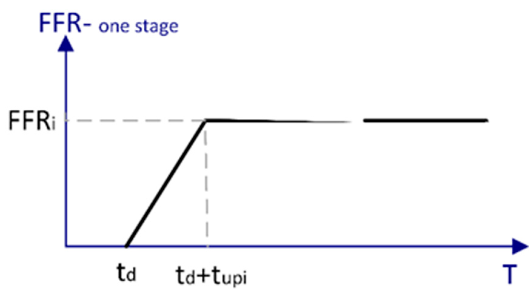
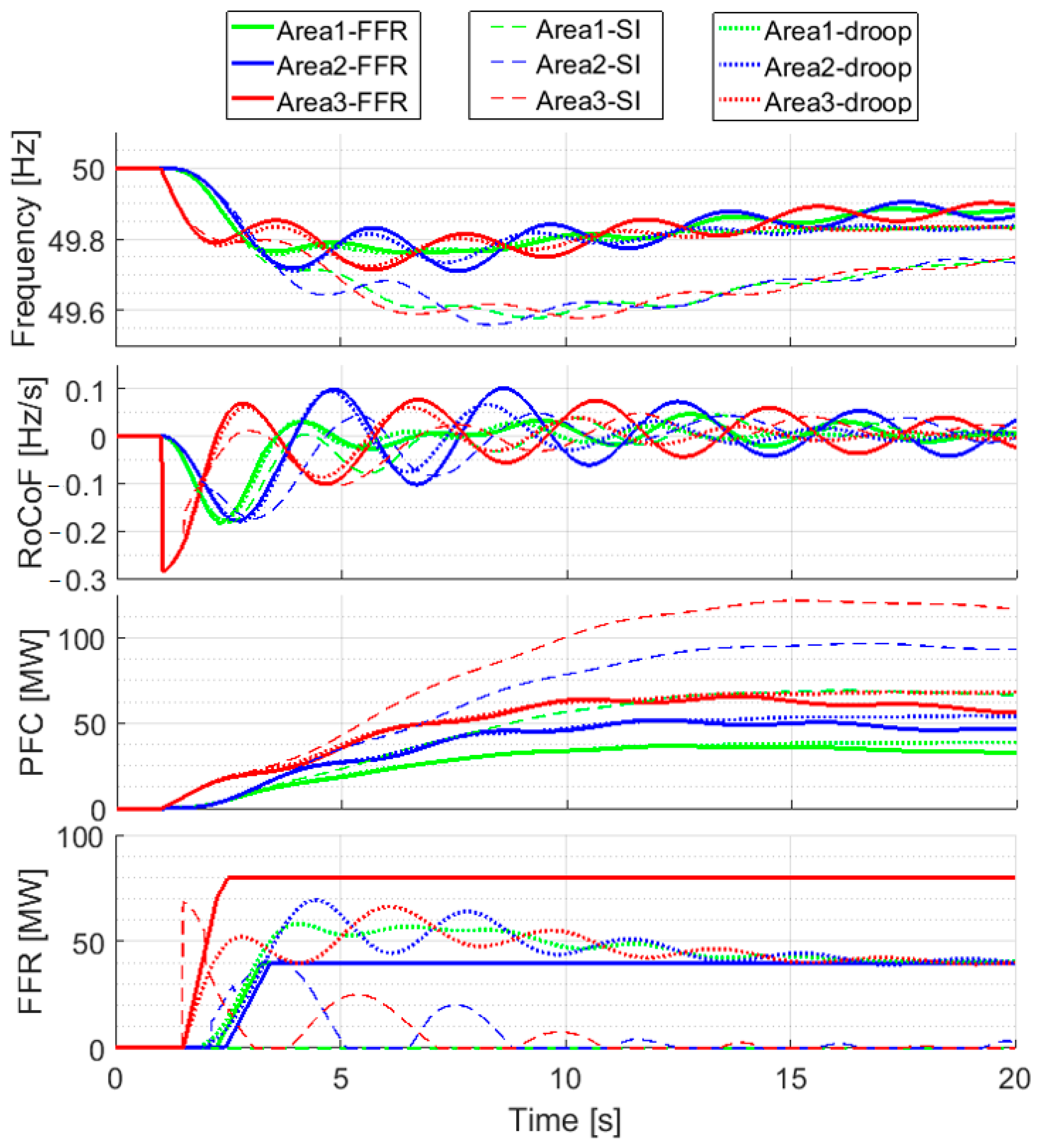
• Contrary to SI and droop-based frequency control, the proposed FFR control delivers constant power in reference to the RoCoF level. Therefore, it effectively utilizes the fast response capability of fast-acting resources and has a bigger contribution towards restraining the frequency nadir.
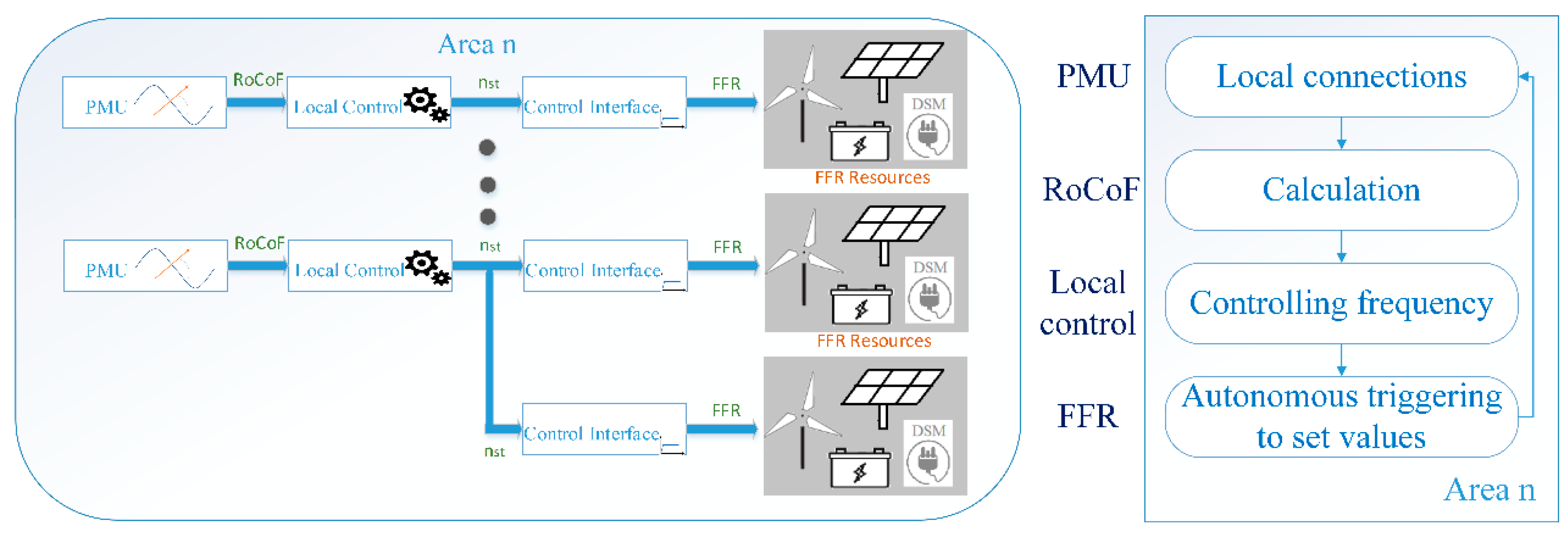
• The proposed frequency control strategy uses only local measurements of the RoCoF. This eliminates the need for placing new and additional communication infrastructure. Most importantly, unpredictable time delays due to data transmissions are avoided, resulting in an even faster and more reliable response of FFR.
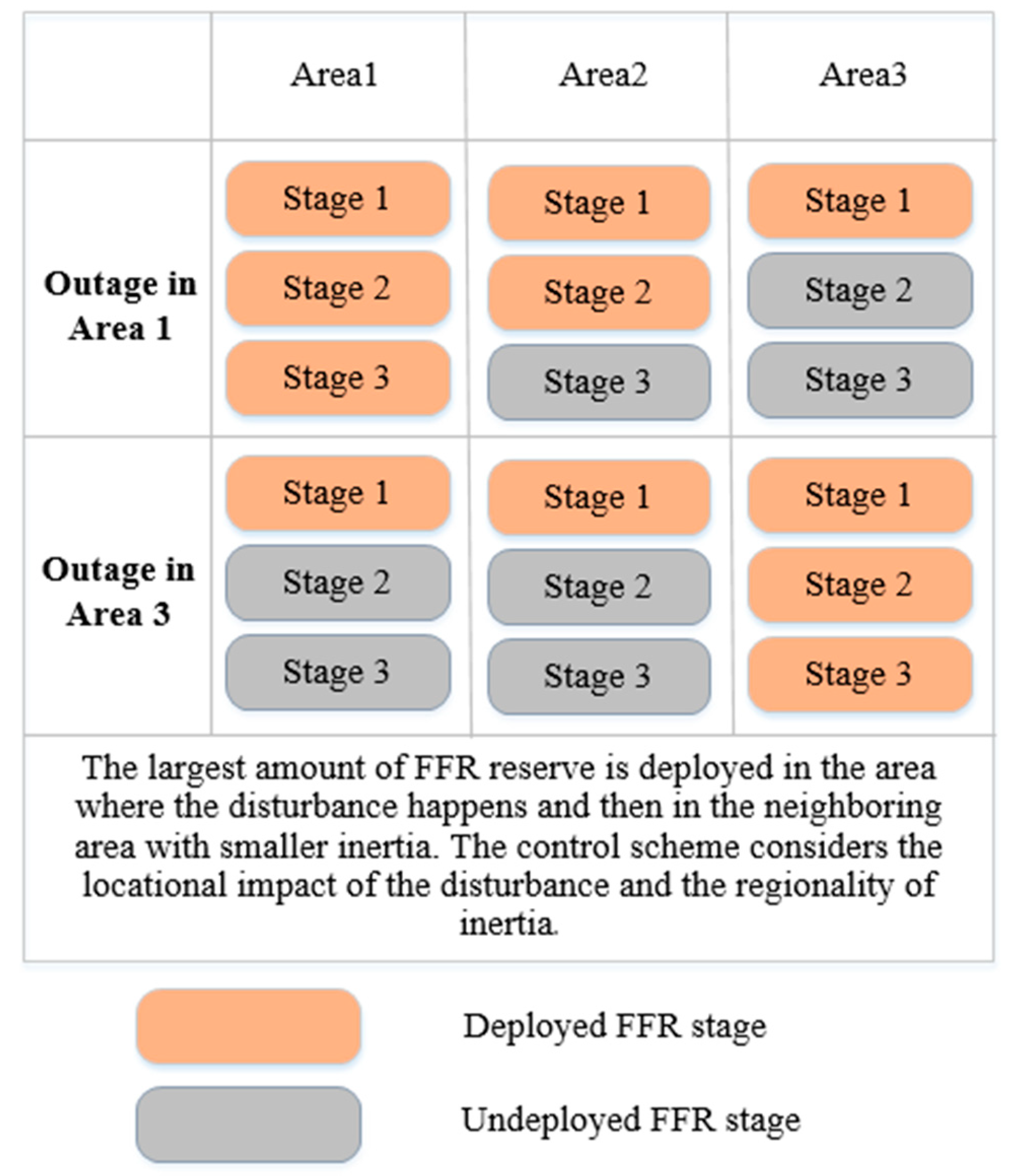
• During the transient period after a disturbance, frequency drops and the RoCoF have the largest values near the location of the disturbance and in low-inertia areas. Consequently, the FFR reserve, which is triggered by locally measured RoCoF, is most deployed in the area where the disturbance occurred, which retains disturbance propagation.
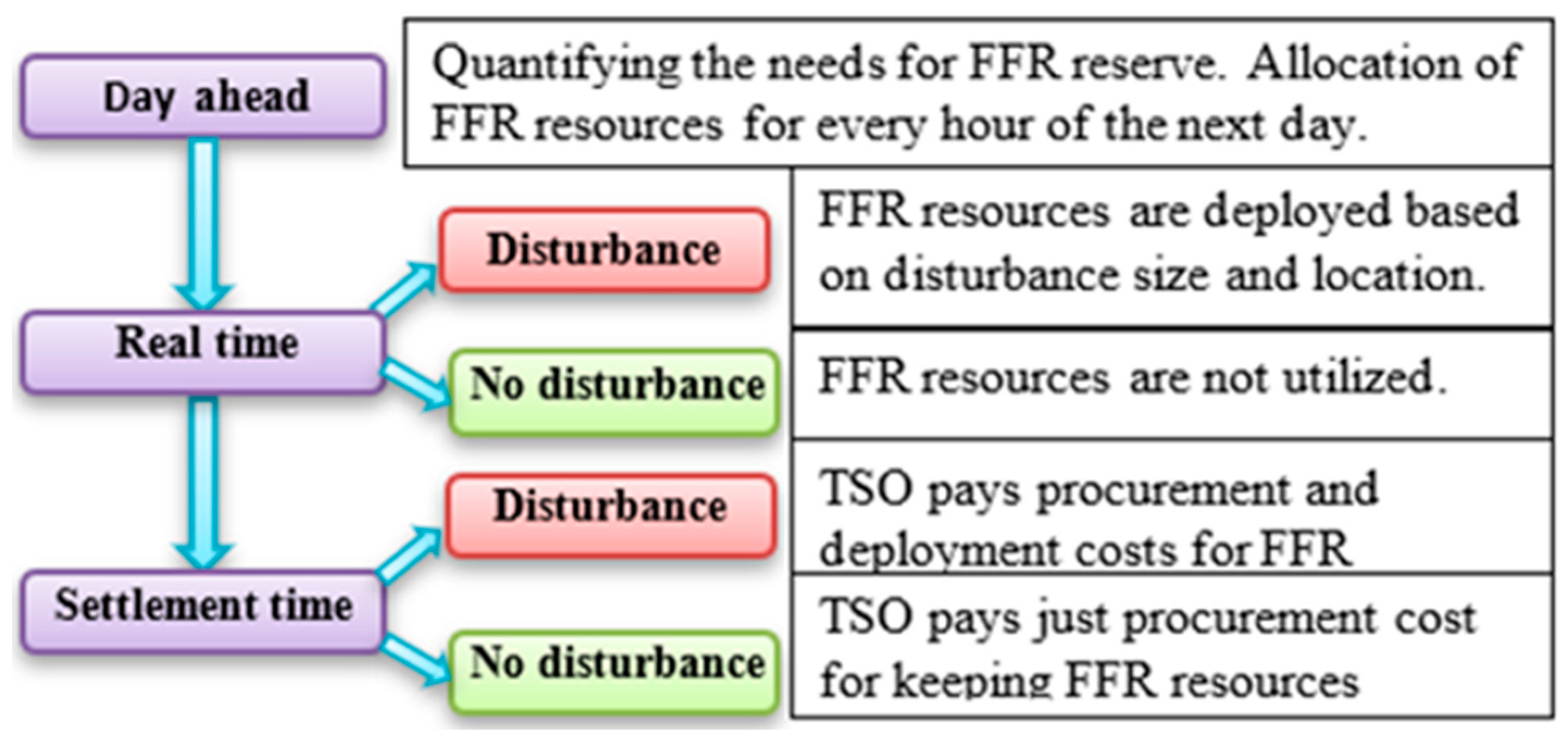
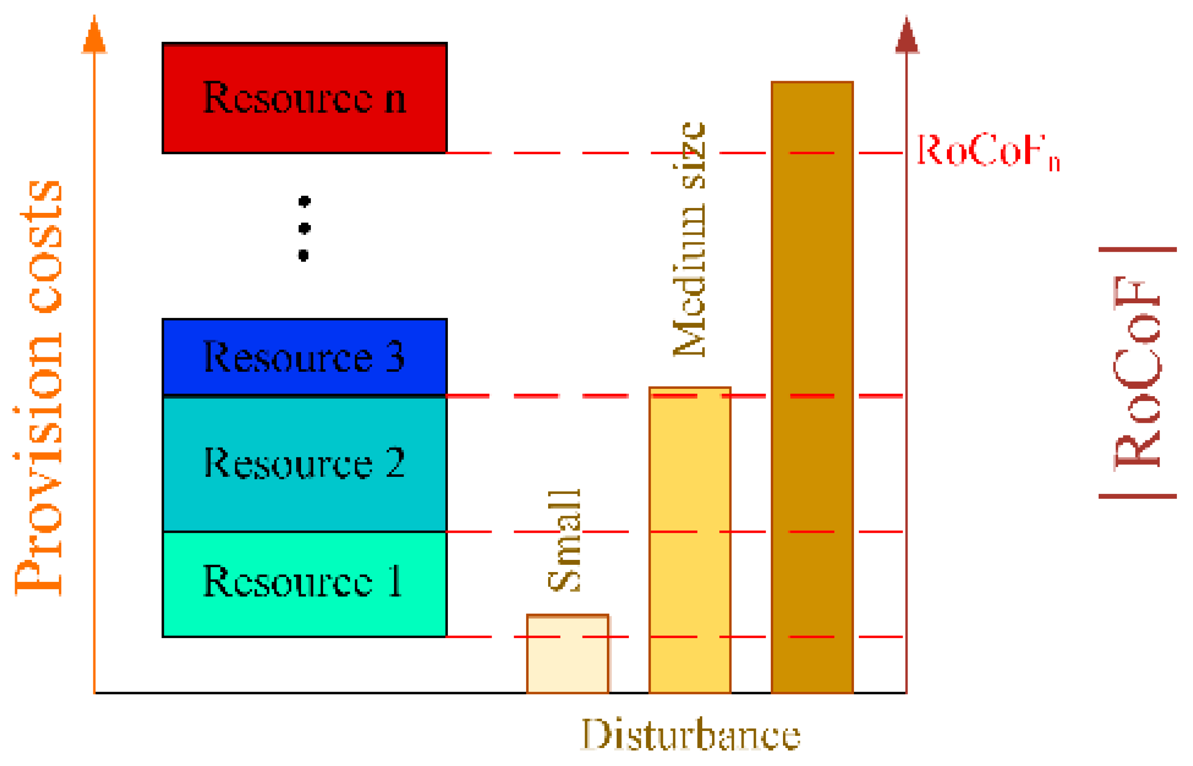
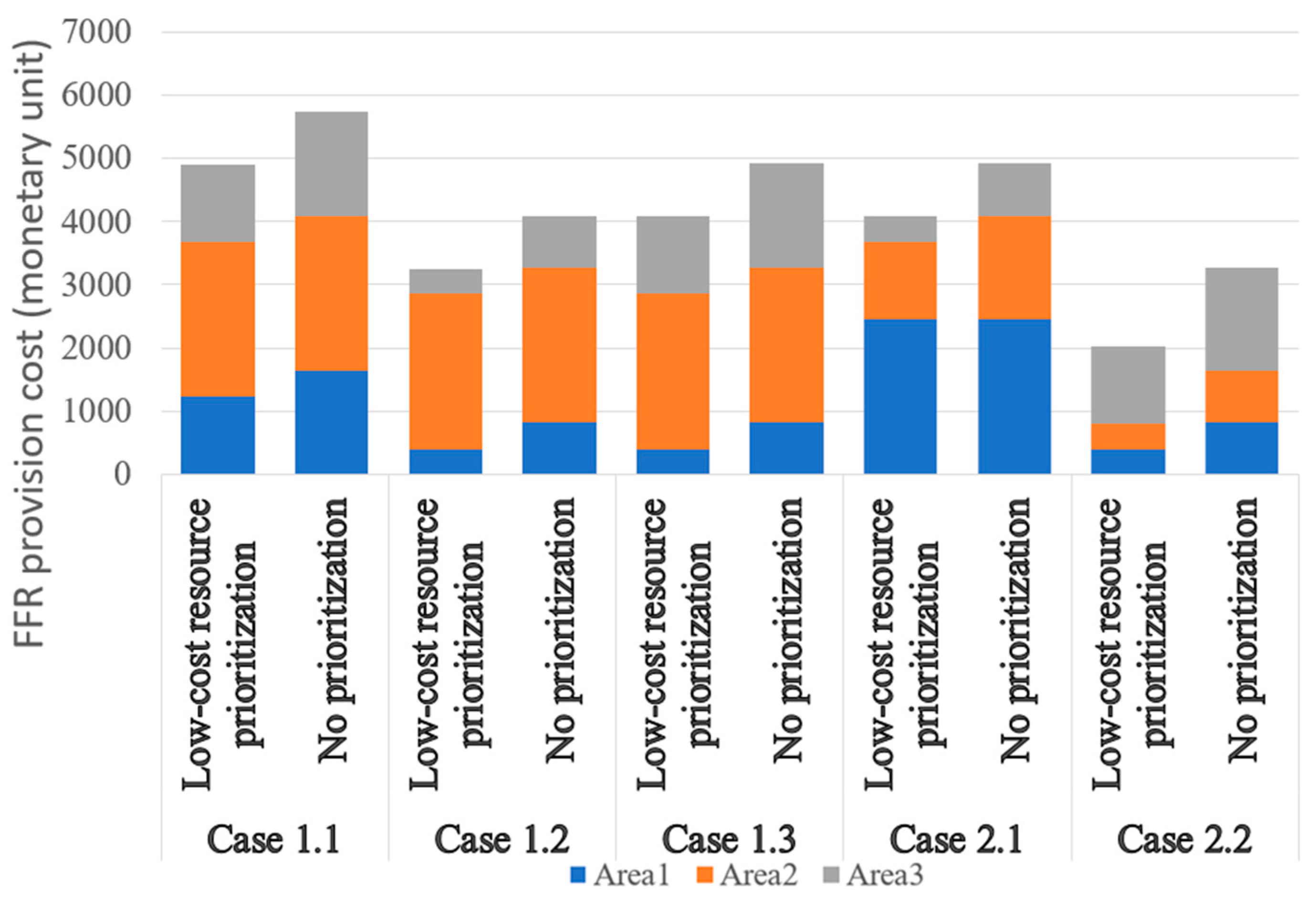
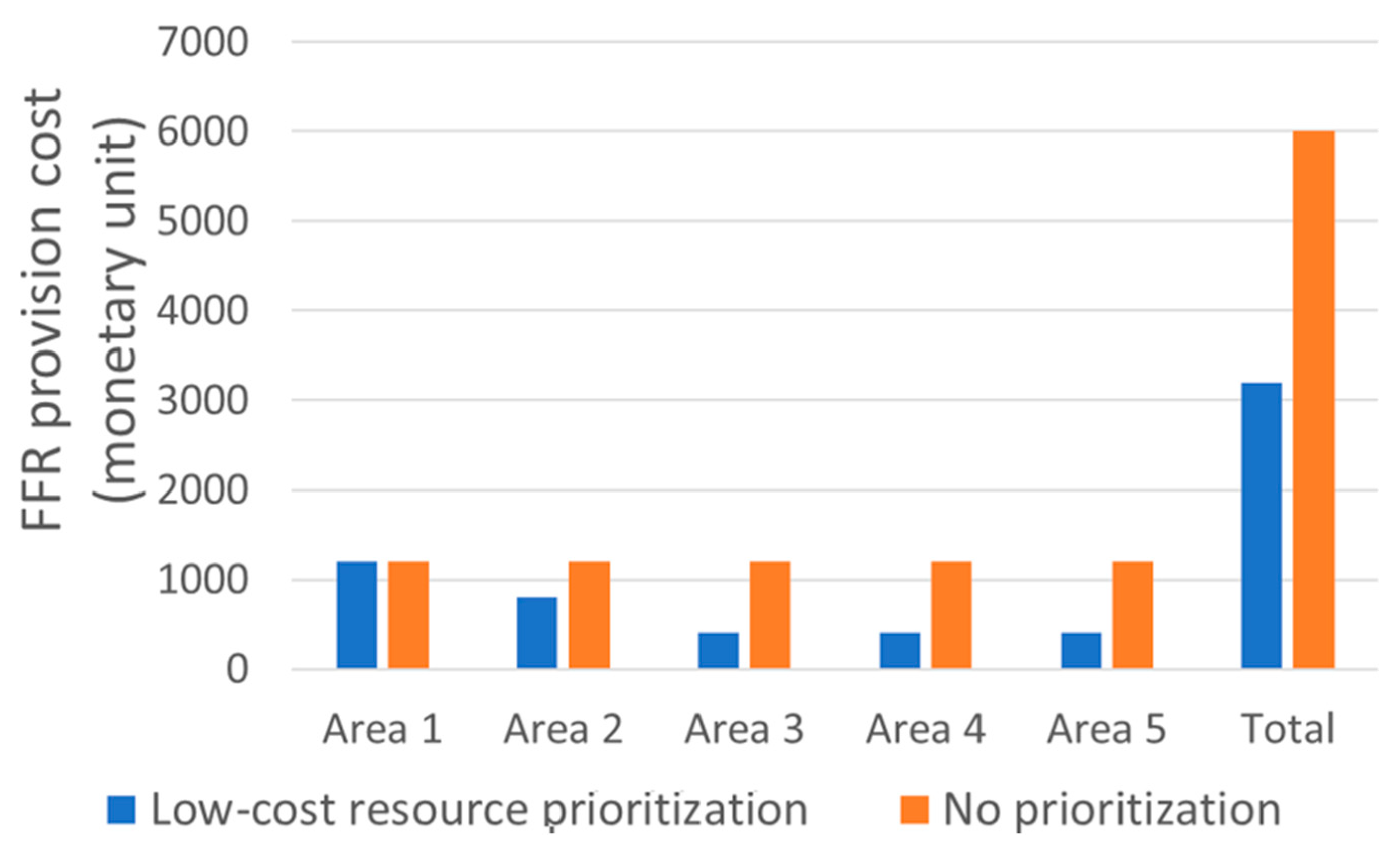
• The proposed multi-stage FFR control strategy ranks reserves based on the provision cost and prioritizes the use of low-cost reserves in case of less severe disturbances. The multi-stage approach gives priority to the low-cost FFR reserve in the case of less critical disturbances and enables TSO to reduce reserve provision costs.

To summarize, the proposed control concept relies on local measurements only and does not need communication infrastructure. Therefore, this solution supports simple and low-cost implementation. The multi-stage principle is introduced as a simple way to deploy reserves proportional to disturbance and to reduce deployment costs for FFR ancillary service. The proposed FFR control scheme considers the non-uniform distribution of inertia in the system and the location of the disturbance. The novelty of the proposed solution lies in the fact that the control strategy can rank different kinds of FFR resources based on location and performance and can prioritize the use of low-cost reserves in the case of less severe disturbances. Its advantage over other methods is the ability to adapt FFR resource response to the disturbance without complex calculations and to minimize the propagation of the disturbance’s impact on system stability.

The proposed FFR control strategy is beneficial for:

• System operators: From an economic perspective, the proposed control strategy reduces provision costs, since the deployed FFR reserves are proportional to the size of the disturbance, and low-cost FFR resources are prioritized. From a technical perspective, the FFR control strategy deploys more reserves in parts of the system that are more affected by disturbances and thus contributes more to frequency stability.
• Consumers: Since the operational costs are mapped to the consumers through the cost of electricity, reduced frequency reserve costs decrease consumer expenses.
• Service providers: The proposed control solution favors FFR resources located in more vulnerable areas (low inertia areas), which can motivate investors to invest in FFR resources in locations that contribute more to system stability. This market-oriented solution leads to efficient investment decisions that can contribute towards a more resilient system.

This paper is organized as follows. Firstly, a theoretical background with a mathematical model is provided. Afterward, the paper proposes the methodology for the FFR control strategy. Then, case studies are described, followed by simulation results and discussion. Finally, closing remarks and future work are presented in the Section 5 and 6.

2. Theoretical Background

This section aims to provide a theoretical foundation that can lead to the basic conclusions of how the FFR control strategy should be designed. For the sake of simplicity, the dynamic model of a two-area system is presented, and the model can be generalized for different configurations of an n-area system. A simplified linearized model of a two-area system can be described by differential equations [33]:

$$\frac{d\mathsf{\Delta }{f}_1}{dt}=\frac{1}{2\times H_1}\left(-K_1^D\mathsf{\Delta }{f}_1-\mathsf{\Delta }P-\mathsf{\Delta }{p}_{12}\right),$$

(1)

$$\frac{d\mathsf{\Delta }{f}_2}{dt}=\frac{1}{2\times H_2}\left(-K_2^D\mathsf{\Delta }{f}_2+{\alpha }_{12}\mathsf{\Delta }{p}_{12}\right),$$

(2)

where Δf₁ and Δf₂ are the relative frequency deviations from the nominal frequencies in areas 1 and 2, respectively, α₁₂ is the areas’ base power ratio and H₁ and H₂ correspond to equivalent inertia constants of areas. The coefficients K₁^D and K₂^D represent the damping coefficient of areas 1 and 2, respectively. The tie-line load flow change Δp₁₂ between areas 1 and 2, following the disturbance ΔP in area 1, can be expressed as:

$$\mathsf{\Delta }{p}_{12}=m_s\times \mathsf{\Delta }{\theta }_{12},$$

(3)

where m_s corresponds to the synchronizing power coefficient, defined as:

$$m_S={\frac{d{P}_{12}}{d{\theta }_{12}}|}_{{\theta }_{{12}_0}}=\frac{U_1^{\prime }{U}_2^{\prime }}{X_{12}^{\prime }}\cos {\theta }_{12},$$

(4)

In Equation (4), U₁′ and U₂′ represent bus voltages at the ends of the tie-line, X₁₂′ is the tie-line reactance and θ₁₂ is the phase angle difference at the ends of the tie-line. The synchronizing power coefficient is inversely proportional to the length of the connecting line. For weakly coupled areas (longer tie-line), m_s has a smaller value.

Equation (3) can be expressed as:

$$\frac{d\mathsf{\Delta }{p}_{12}}{dt}=m_s\left(\mathsf{\Delta }{f}_1-\mathsf{\Delta }{f}_2\right),$$

(5)

A system of first-order differential Equations (1), (2) and (5) represents the dynamic model of a two-area interconnected power system. This simplified model does not include a change in generator power output due to the primary frequency response, since the time interval of interest for FFR is only a few seconds after a disturbance. The adopted assumption is reasonable because the generators providing primary response services need time to ramp up and increase their power output. FFR is expected to be activated in one second after a disturbance.

For simplicity, and without significant loss of generality, it was adopted that α₁₂ = 1 and K₁^D/H₁ ≈ K₂^D/H₂, which provides the possibility of finding analytical solutions to the system of differential equations.

With the assumption that the frequencies in areas 1 and 2 are equal to the nominal value before the disturbance, the frequency responses have the following analytical form:

$$\Delta f_1=\left(\frac{H}{4H_1^2\delta }-\frac{1}{4H_1\delta }\right)\mathsf{\Delta }P\left(1-e^{-2\delta t}\right)-\frac{H}{2H_1^2\omega }\mathsf{\Delta }P{e}^{-\delta t}\sin \omega t,$$

(6)

$$\Delta f_2=-\frac{H}{4H_1{H}_2\delta }\mathsf{\Delta }P\left(1-e^{-2\delta t}\right)+\frac{H}{2H_1{H}_2\omega }\mathsf{\Delta }P{e}^{-\delta t}\sin \omega t,$$

(7)

In expressions (6) and (7), symbol H represents equivalent inertia constants of a two-area system, defined as:

$$H=\frac{H_1{H}_2}{H_1+H_2} ,$$

(8)

ω is the frequency of inter-area oscillations:

$$\omega =\sqrt{\frac{m_s}{2H}-{\left(\frac{K_1^D}{4H_1}\right)}^2},$$

(9)

where Δ represents a damping coefficient of inter-area oscillations, defined as:

$$\delta =\frac{K_1^D}{4H_1} .$$

(10)

Considering the fact that the tie-line load flow change Δp₁₂ at the initial moment is equal to zero, the initial value of the RoCoF in area 1, where the disturbance occurred, can be calculated using Equation (1), and it depends only on the magnitude of the disturbance and the inertia of that area:

$${RoCo{F}_1}_0=\frac{\Delta P}{2\times H_1},$$

(11)

The initial value of the RoCoF in area 2, based on Equation (2), is equal to zero.

The RoCoF in area 1 is the largest in the initial moment (frequency declines after a disturbance and the RoCoF has a negative value, but we used the terms that are the largest and the maximum related to the absolute value of RoCoF), and the largest value of the RoCoF in area 2 and the moment when it occurs depend on inertia distribution, the value of the synchronizing power coefficient (distance from the location of the disturbance) and the damping coefficient. The maximum values of the RoCoF in area 1 and area 2 and in the moment when it occurs, depending on inertia distribution, are presented in Figure 1. If area 2 has smaller inertia than area 1, the maximum value of the RoCoF in area 2 is greater than in the case when area 2 has bigger inertia than area 1. Low-inertia area 2 is also affected by the disturbance sooner than the high-inertia area, which is identically distant from area 1.

Figure 2 shows the maximum absolute value of the RoCoF in area 1 and area 2, as well as the moment this value occurs depending on area distance, i.e., the value of synchronizing power coefficient. As seen in Figure 2, in a weaker-connected system, the difference in the maximum values of the RoCoF in areas 1 and 2 is larger than in a stronger-connected system, and it takes more time to reach the highest value of the RoCoF in area 2, as well. The results demonstrate that more distant areas are affected by the disturbance later and with less intensity than the closer ones.

The influence of the dumping coefficient on the maximum values of the RoCoF is negligible and therefore is not shown here.

The difference in the frequency responses of areas 1 and 2 is dictated by inter-area oscillations, and these differences enable spatially dependent local frequency control. In the short period immediately after the disturbance, there is still no significant effect of primary frequency control, and accordingly, the turbine regulator is omitted in the considered model. Moreover, the existence of a power system stabilizer does not affect the differences in frequency responses in the time frame of a few seconds immediately after the disturbance. Therefore, further analysis can be limited to the evaluation of the influence of synchronizing power coefficients and inertia distribution as key factors influencing the frequency and amplitude of inter-area oscillations.

The frequency of inter-area oscillations, depending on inertia distribution, and synchronizing power are shown in Figure 3; Figure 4, respectively. The graphics show that, in the case of weak interconnection, the inter-area frequencies are lower compared to the case of strong interconnection, in which areas are less distant. Lower inter-area frequencies are also experienced in the case when area 2 has bigger inertia than area 1.

The values of the RoCoF in areas 1 and 2 for different frequencies of inter-area oscillations are presented in Figure 5; Figure 6, respectively. With smaller frequencies of inter-area oscillations, there are greater differences in the values and time delays of the areas’ RoCoF, whereas with higher frequencies of inter-area oscillations, RoCoF changes are transmitted much faster in other parts of the system. The FFR control strategy can use these delays in the appearance of the RoCoF; therefore, the fastest and largest FFR is performed in the area where the disturbance occurred, before activating FFR in other areas. The obtained results indicate that, shortly after the disturbance, frequency and RoCoF differ more in the less connected areas, and it takes more time for the frequency to become uniform in the entire interconnection.

Such results are in favor of the FFR that is triggered by the RoCoF value because the resources that are closer to the disturbance respond sooner. The analysis also confirms that the neighboring area of lower inertia is affected by the disturbance sooner and that the RoCoF is higher compared to the neighboring area of higher inertia. This conclusion is positive from the perspective of FFR activation because resources in low-inertia parts of the system, which are also more endangered by disturbances, are dispatched more quickly and in greater numbers.

3. A Novel Approach for the Implementation of Fast Frequency Control in Low-Inertia Power Systems Based on Local Measurements and Provision Costs

The conclusions from the previous section indicate that differences in frequency responses in different parts of the system, within the first few seconds following the disturbance, allow spatially dependent activation of FFR that is based only on local RoCoF measurements. Therefore, FFR service providers located in different nodes do not need to exchange information and can act completely independently. Consequently, this eliminates the need for placing new communication infrastructure and enables prompt responses, as there are no unpredictable time delays due to data flow. Since the control decision is made on the resource side, the delays are determined only by the FFR response delay, the limitations of the control loops and the FFR resource itself. In the worst case, when the measurement is not performed at the connection point of the FFR service provider, the delays that must also be anticipated relate to the transmission of the RoCoF signal from the nearest measurement point in the system to the FFR service provider itself. With this concept, it is also easy to integrate new FFR service providers in different nodes. An overview of the FFR control strategy for one of the areas of the power system is illustrated in Figure 7. As shown in Figure 7, the area can have many different FFR resources (energy storage, PVs, wind turbines, demand response, etc.) located in different nodes of the area. Each FFR resource gets RoCoF measurements from the nearest PMU device, and the same PMU device can be used for more than one FFR resource. FFR reserves are divided into stages that are or are not dispatched, depending on the RoCoF value obtained by the associated PMU device and the defined threshold levels for FFR stage activation.

Each resource providing the FFR has one local controller and PMU device connected at the same or close connection point. The transmission network is divided into coherency zones (areas) that experience similar frequency behavior during disturbances (Figure 8). To this end, the necessary step in designing the FFR control scheme is to determine coherent areas based on the analysis of system dynamics.

In this case, coherence is related to the PMU measurements and not to the generators’ behavior, so the coherence can be measured by the time delay between the occurrence of the RoCoF maximum at the measurement points in the system. This criterion defines a coherent zone as an area in which these differences are less than the given values. The identification of a cluster of busses with similar frequency behavior following a disturbance in the system is presented in [34] using a coherency identification technique based on a Wide Area Measurement System that is robust in the presence of noise in the measured signal. In this way, the spatial distribution of resources that are expected to be activated after a disturbance in some part of the system is defined. The FFR reserves in the area of the disturbance are activated immediately. The FFR reserves in other areas are activated later or not activated at all, since they may experience delays in RoCoF behavior compared to the RoCoF in the area of the disturbance. In addition, it should be considered that the activation of the FFR reserve in the area of the disturbance immediately after the event dynamically reduces the need for FFR activation in other areas. In this way, the reserve closer to the disturbance is predominantly used and thus reduces changes in power flows in the system as well as the stability problems that accompany them. At this point, it must be stressed that we can give a basis to determine the significance to FFR resources by activation closer to the disturbance, and this can be further used in frequency deviation optimization procedures, such as in [32]. This is an additional value of this paper.

The total required FFR control reserves in the system are determined for the case of the most critical disturbance to keep the frequency above the defined limit. To adjust the required level of activated reserves in less critical situations, FFR resources are apportioned in N_st stages that are triggered at different values of the RoCoF. Stage FFR_i is triggered if the RoCoF value is greater than RoCoF_i, and it is fully deployed after time t_upi after the activation. t_d is the time needed for reliable measurements of the RoCoF and the delay in FFR onset. The provision of the FFR is assumed to linearly increase with time until it reaches a constant value (Figure 9):

$$FFR\left(t\right)={{\displaystyle \sum }}_{i=1}^{N_{st}}FF{R}_i\left(t\right) ,$$

(12)

$$FF{R}_i\left(t\right)=\{\begin{array}{cc}0& RoCoF\left(0_{+}\right)<RoCo{F}_i\\ FF{R}_i^a\left(t\right)& RoCoF\left(0_{+}\right)\ge RoCo{F}_i\end{array},$$

(13)

$$FF{R}_i^a\left(t\right)=\{\begin{array}{cc}0& t<t_d\\ \frac{FF{R}_i}{t_{u{p}_i}}\times \left(t-t_d\right)& t_d\le t\le t_{u{p}_i}\\ FF{R}_i& t>t_{u{p}_i}+t_d\end{array}+t_d,$$

(14)

Although a smaller number of FFR stages provides simpler control that is easier to implement, a larger number of FFR stages frequency support that is more tailored to the disturbance. The number of stages is limited by the requirement that the FFR control should be fast and that all stages should be activated well before the frequency reaches nadir (usually of the order of a few seconds). On the other hand, the requirements of selectivity of multi-stage control are determined by the differences in frequency responses of individual parts of the system conditioned by inter-area oscillations. The difference between the stages is the FFR ramp-up rate and the RoCoF threshold value for activation. The first stage is activated at the lowest RoCoF threshold value, and it is the slowest one. The second FFR stage is activated at a higher value of RoCoF, and it is faster, i.e., it takes less time to reach the full capacity of the allocated stage reserve than the first stage. Each following stage is activated at higher RoCoF values, and each stage is faster than the previous one. The last FFR stage is the fastest one, and it is triggered by the highest RoCoF value. In this way, the multi-stage solution provides that, in the case of smaller disturbances and smaller values of RoCoF as well, slower (and assuming cheaper) FFR reserves are dispatched because the frequency stability is less compromised.

The number of FFR stages is not uniform, and it varies depending on the location of the resource and the volume of the existing reserve. In areas with low inertia, the number of degrees should be greater, as such locations are more sensitive to disturbances. RoCoF threshold levels are pre-defined based on a day-ahead dispatch plan. The number of stages and thresholds is defined by the TSO, and a comprehensive evaluation of those values is out of the scope of this paper. A detailed assessment of the power system may inspire practical criteria for the definition of threshold values and corresponding reserves to be activated.

Although the total FFR reserve in the system is determined based on the most critical expected disturbance in the whole system, the reserve in each area is determined based on the desired share in covering the expected critical event in the area. Each area has a targeted amount of response and a defined sequence for FRR resources to be deployed. Having multiple stages dispatched at different values of RoCoF is the way to define the order in which FFR resources are dispatched.

The RoCoF threshold value for the last stage of FFR in the area is determined considering the expected magnitude of the disturbance in the area and the inertia constant of the area, using Equation (11). The RoCoF value obtained by this expression is the maximum expected RoCoF for disturbance in that area, as shown in Figure 1; Figure 2. The RoCoF threshold value for the last stage of FFR in the area should be slightly less than the expected maximum RoCoF, provided that all FFR stages (full reserve) are dispatched in the case of the most critical disturbance. The optimal RoCoF threshold values for other stages of FFR should be calculated with day-ahead scheduling and reserve planning, and they require detailed system data and a list of potential outages. For each potential disturbance in that area, the frequency response should be analyzed for the forecasted operating state, and the maximum RoCoF as well as the needed FFR reserve should be obtained. Using the statistical analyses, the optimal RoCoF threshold values for other stages can be calculated to provide FFR support that is suitable to the size of the disturbance. It should be pointed out that RoCoF threshold values can be adjusted on an hourly basis to provide the most adequate response for possible disturbances, since the operating state and inertia distribution vary over time. Nevertheless, the simple method used when RoCoF threshold values are chosen to be equidistant can also provide a response that is relative to the size of the disturbance, since the maximum RoCoF is proportional to the size of the disturbance (Equation (11)).

Based on analyses provided in the previous section, the proposed multi-stage FFR control strategy that is triggered by RoCoF ensures that more FFR reserves can be activated in systems with less inertia as well as in the area closer to disturbance. It also provides that, in the strongly coupled parts, the simultaneous activation of the reserve ensures more even distribution of frequency support.

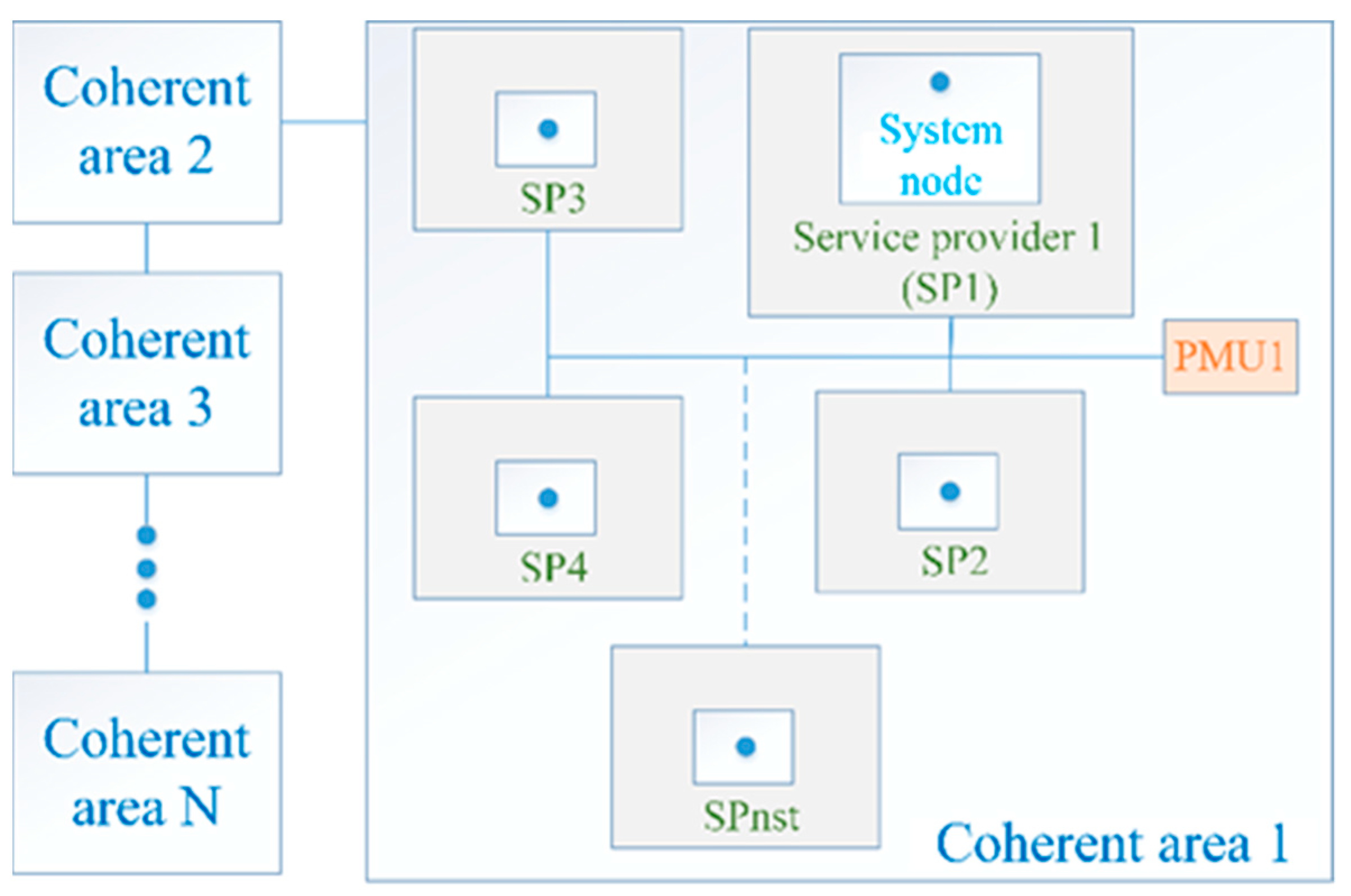
Potential FFR Market Structure That Enables Ranking FFR Resources Based on Reserve Provision Costs

FFR service markets must be designed and the cost of provided service should be determined through this market mechanism. It is important to design a proper FFR control strategy to ensure system security first and then to base market structures on that foundation. The market design should allow TSOs to pay for the reservation of reserve capacities. Participants offer a capacity price bid and a mileage price bid, and then the system operator credits the participants. In such an arrangement, winning resources are obligated to provide FFR service when called upon, in return for a fixed revenue stream. Payments can also include the energy delivered element if the FFR resource is utilized. Figure 10 shows the timeline and cost associated with the FFR service. In day-ahead planning, TSO quantifies the needs for FFR reserve and allocates the FFR resources for every hour of the following day. During real-time operations, FFR resources are deployed in the case of a disturbance; otherwise, they are not utilized. If a disturbance happens, the TSO pays the procurement and deployment costs for FFR service in settlement time; if not, the TSO pays just procurement costs for keeping FFR resources reserved. A market organized in this way allows the TSO to prioritize the appropriate FFR resources depending on the price for energy delivered. FFR provision cost can be used as a criterion to rank FFR resources in a merit order system based on an ascending order of price, prioritizing resources that are less expensive; therefore, the TSO can reduce costs for FFR control ancillary service. Having a multi-stage approach instead of a one-stage approach provides more suitable FFR support proportional to the size of the disturbance, but it also has economic benefits. The proposed multi-stage FFR control strategy in which different stages are triggered at different values of RoCoF enables the incorporation of a merit order system by assigning different FFR reserves to the stage based on its rank (Figure 11). Less expensive FFR reserves are prioritized and are activated at lower RoCoF values, and they are dispatched in the case of less critical disturbances. More expensive FFR reserves are dispatched at higher RoCoF values only in the case of severe disturbances. In this way, the TSO can cut costs related to FFR provision.

4. Case Studies and Simulation Results

The performance of the proposed FFR control strategy is validated through computer-based dynamic simulations of a simple three-area power system and an IEEE 68-bus system. A three-area power system model is used to test the performance of the FFR in a multi-area system for different grid strengths and different levels and regionalities of inertia. The simulations performed using this system are intended to give basic insight into the spatial activation of FFR after a disturbance and to provide an indication of the influence of FFR resource location. Furthermore, the simulations on the IEEE 68-bus system should confirm the applicability of the proposed control strategy in complex power systems.

The system and frequency responses in various scenarios were simulated using MATLAB/Simulink. It should be noted that the secondary frequency control to restore system frequency to nominal values is not of relevance in these analyses and was not implemented in the simulations. This service is usually activated within 2–15 min after the frequency deviation, and the FFR is an emergency service that ensures that frequency does not collapse after a severe contingency. Therefore, only primary frequency control is implemented by applying a corresponding droop coefficient to the generator model. It should be emphasized that the activation times of the FFR provider were not considered, and time delays only relate to the length of measurement windows, which are the same in every simulation and are equal to 500 ms. At this point, we did not consider the impact of different delays imposed by PMU measurements or the noisy impact of the derivative action to obtain the RoCoF. Regarding FFR resource capabilities, the ramp-up rate is demonstrated to be the most important one, and the response delay does not appear to be very significant [22].

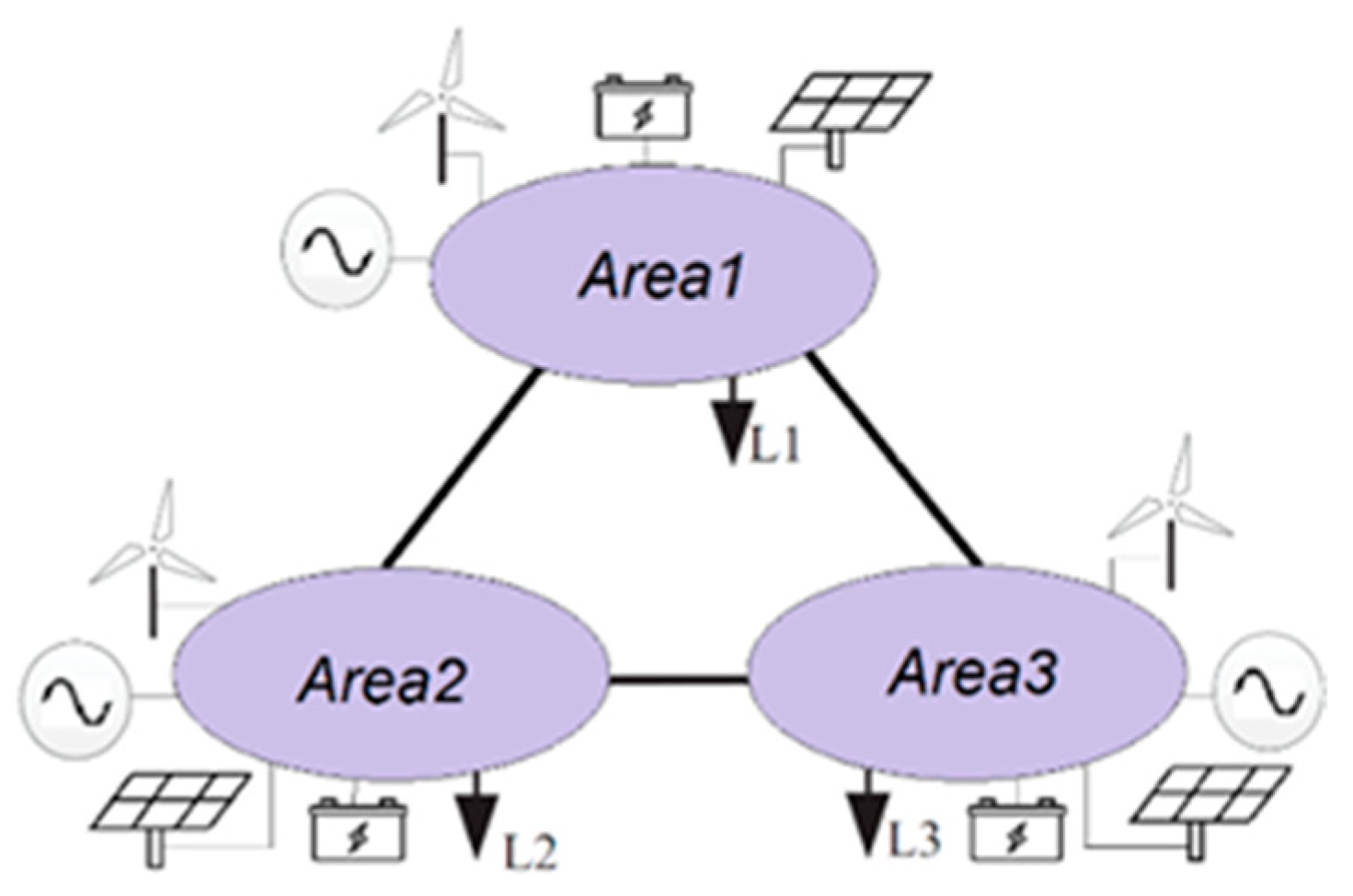
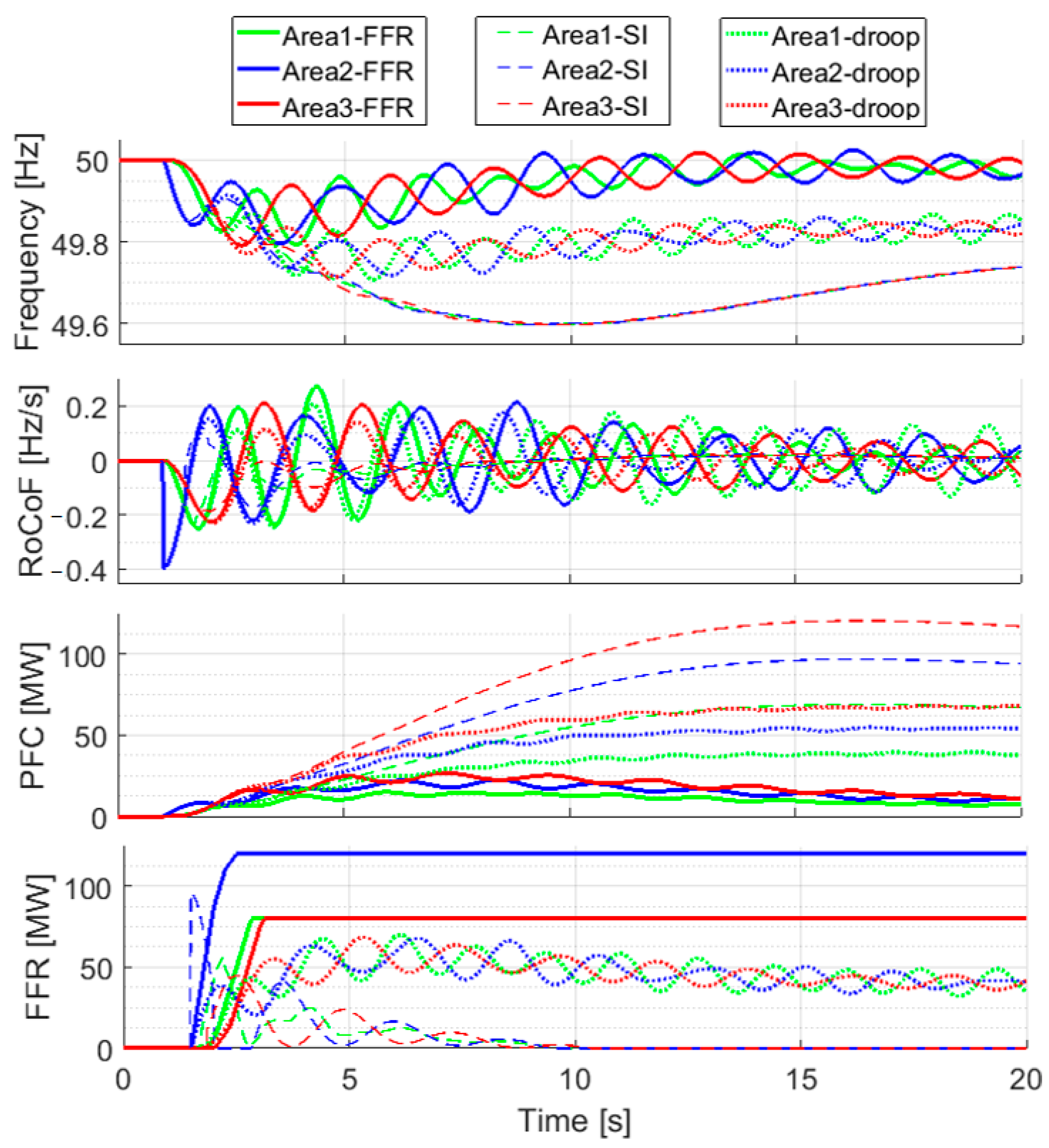
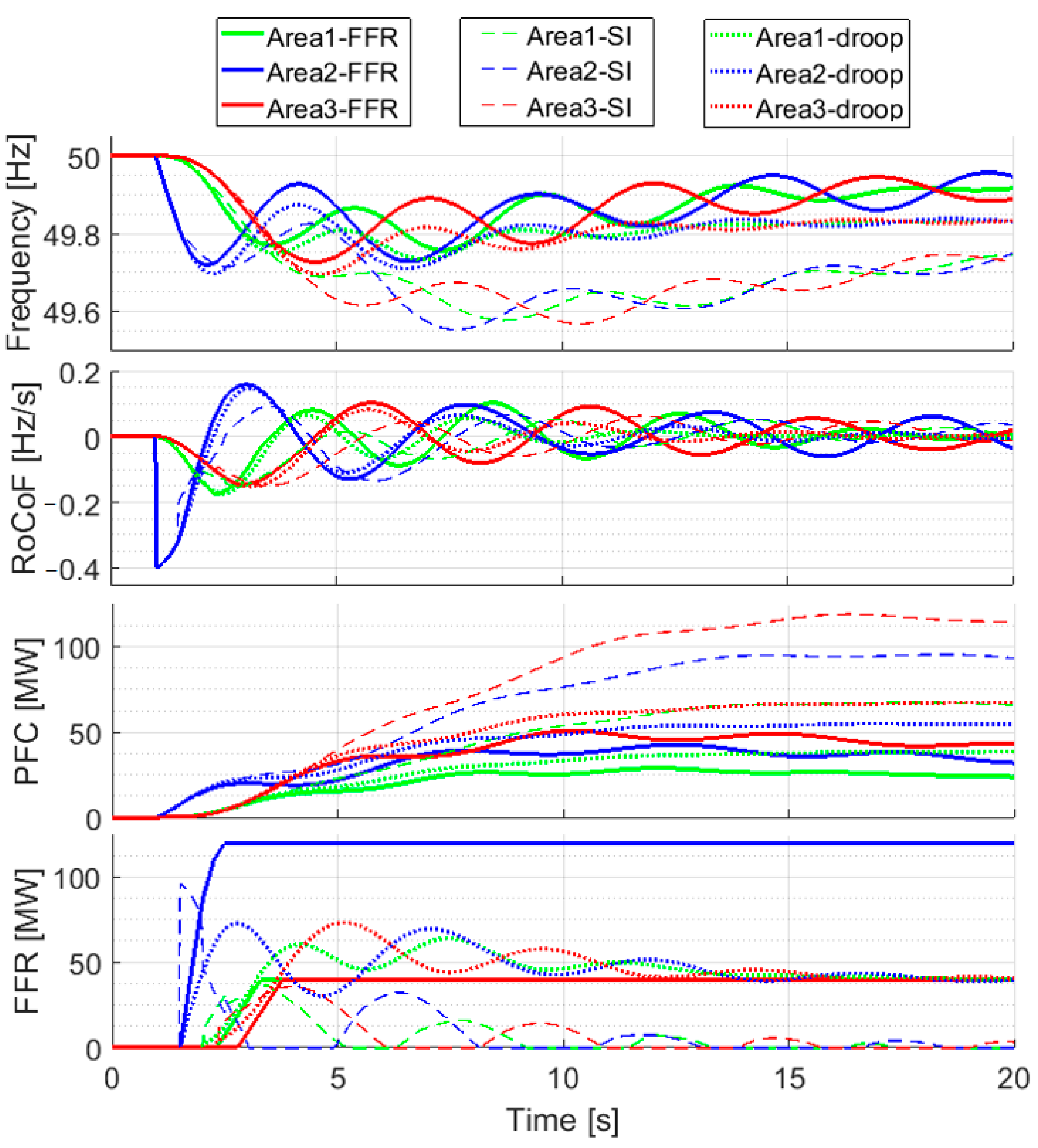
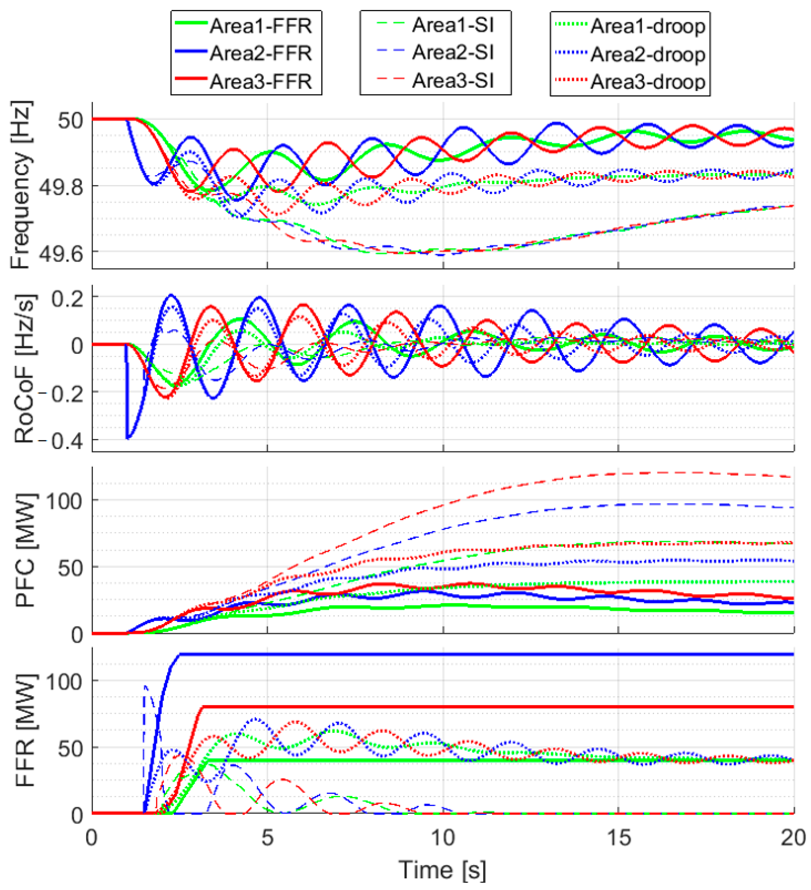
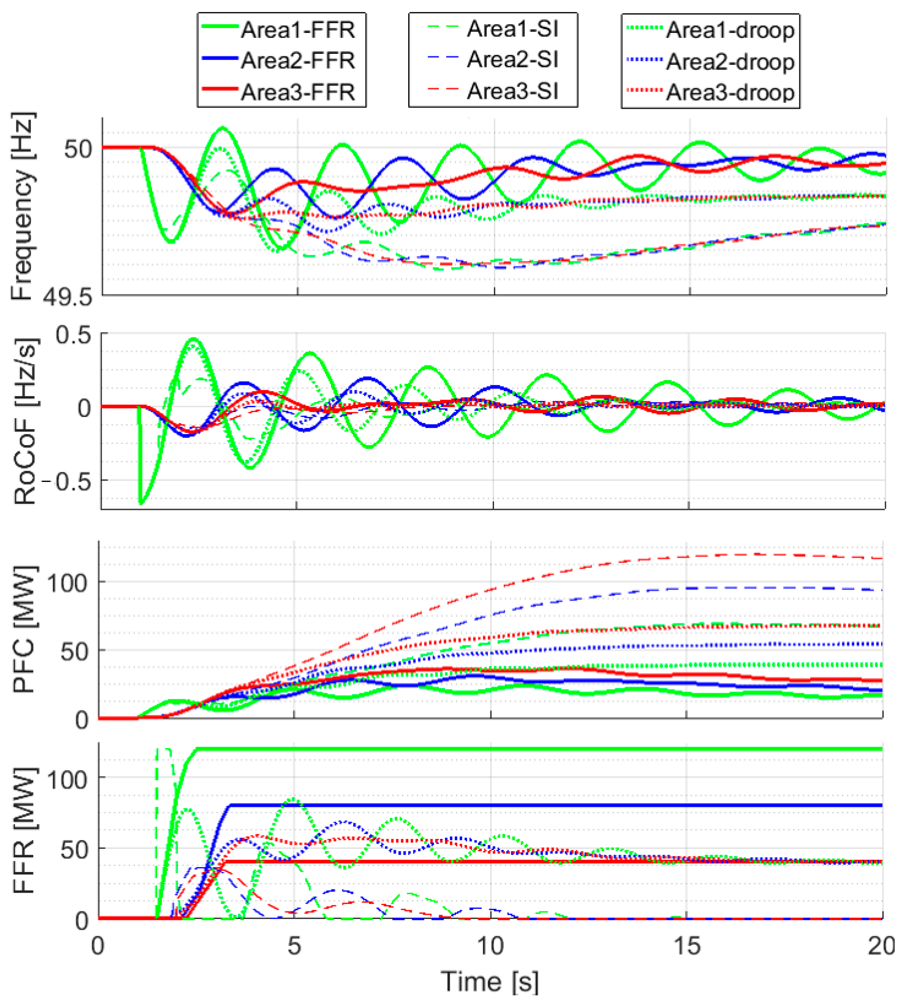
4.1. Simulations on a Simple Three-Area System

A generic three-area test system was created, as displayed in Figure 12. Each area has aggregated synchronous generation, non-synchronous generation, load and FFR and is represented as a low-order System Frequency Response (SFR) model [35]. The test system was created to be representative of a future low-inertia system considering the heterogeneous distribution of inertia in the system. Area1 represents a low-inertia part of the system where non-synchronous generation comprises 70% of the load, and Area2 has a 50% share of non-synchronous generation, whereas Area3 has a 30% share.

The important parameters for each area are given in

Table 1. Three-area test system data.

Area	Demand [GW]	FFR [MW]	Inertia [s]
Area1	4	120	3
Area2	4	120	5
Area3	4	120	7

. Without the loss of generality, it was adopted that all areas have the same demand and the same amount of FFR reserves. The modelled FFR is representative of an aggregation of multiple FFR services, and, in this step, the focus is not on the resource providers and characteristics of response as response delay, ramp-up rate and FFR capacity. It should be noted that the number of FFR stages and RoCoF threshold values are not of significant importance in these studies. In practical circumstances, the number of stages and RoCoF threshold values should be determined based on the system state before a disturbance. The difference between the stages is the FFR ramp-up rate. In the simulations, different provision costs were incorporated within different ramp-up rates, assuming that a slower reserve costs less, as shown in

Table 2. Multi-stage FFR parameters.

FFR Stage	Activated at RoCoF [Hz/s]	Fully Available in [s]	Provision Price [€/MWs]
1	0.1	1	1
2	0.2	0.75	2
3	0.3	0.5	3

. The first stage activates at the lowest value of the RoCoF, and it takes more time to reach the full capacity of the allocated stage reserve, whereas the last FFR stage is the fastest one. In this way, the multi-stage solution provides that, in the case of smaller disturbances and smaller values of the RoCoF as well, slower (cheaper) FFR reserves are dispatched because the frequency stability is less compromised. It should be pointed out that the RoCoF threshold value for the last stage of FFR is defined based on Equation (11), according to the largest magnitude of the expected disturbance in that area and the inertia of that area. RoCoF threshold values for other stages of FFR are chosen to be equidistant since the precise definition of the optimal RoCoF threshold values require comprehensive analyses of frequency response for all potential disturbances, and this will be conducted in further research. Moreover, the number of FFR stages was arbitrarily chosen, and it was guided by the assumption that it was large enough to show the selectivity of the FFR reserve and the advantages of the multi-stage method and yet not too large to make the results clearer.

To investigate the influence of distance from the location of the disturbance on FFR, three system configurations were developed:

• Case 1.1: Strongly coupled areas;
• Case 1.2: Weakly coupled areas;
• Case 1.3: Different lengths of connection lines.

It should be noted that the term Strong/Weak grid in the manuscript is related to grid strength with respect to strongly/weakly coupled grids. Strongly coupled grids have shorter connection lines, and areas are electrically closer compared to weak grids, where areas are more electrically distant.

The relevant values are presented in

Table 3. Simulation data for determining the impact of grid strength.

Case	1–2 Line Length [p.u.]	1–3 Line Length [p.u.]	2–3 Line Length [p.u.]	Size of Disturbance [MW]	Location of Disturbance
1.1	1	1	1	320	Area2
1.2	5	5	5	320	Area2
1.3	5	3	1	320	Area2

. Configurations differ in line lengths, and the same disturbance was simulated in the medium-inertia area.

Figure 13 shows a 3-area test system response in the case of a disturbance in Area2, when the grid is strong, i.e., the connecting lines are short. The RoCoF was the largest in the area of disturbance, and it was equal to 0.400 Hz/s. Area1 and Area3 experienced the disturbance later, and the largest RoCoF values happened half a second later, which were equal to 0.246 Hz/s and 0.227 Hz/s, respectively. The frequency nadir was the biggest in Area1, where the frequency reached 49.79 Hz but was very similar in other areas. Regarding the amount of activated FFR reserves, in Area2, where the disturbance happened, three stages of FFR were dispatched, whereas in neighboring areas only two were dispatched. Nevertheless, SI and droop control resulted in lower frequencies compared to the proposed multi-stage FFR control. Moreover, droop control does not recognize the location of the disturbance and provides a similar response in all areas. SI control provides the biggest support in the area of disturbance, but its support diminishes fast, since the RoCoF sets off towards zero after a disturbance. As a result, primary frequency control is dispatched more in the case of SI as well droop control.

The test system response in the case of an identical disturbance when the areas were weakly coupled is shown in Figure 14. The RoCoF was the largest in the area of the disturbance, and it was equal to 0.400 Hz/s. Area1 and Area3 experienced the disturbance afterwards, and the largest RoCoF values happened about one second later, which were equal to 0.174 Hz/s and 0.143 Hz/s, respectively. The frequency nadir was the biggest in Area2, where the frequency reached 49.72 Hz. Regarding the amount of activated FFR reserves, in Area2, where the disturbance happened, three stages of FFR were dispatched, whereas in neighboring areas only one was dispatched. Comparing cases 1.1 and 1.2, it can be concluded that, although the size and location of the disturbance were the same in both studies if the grid was stronger, areas’ frequency responses were more similar. On the other hand, a weaker grid resulted in greater differences in frequency responses from individual areas. As a result, less FFR reserves were dispatched, and the area of the disturbance took over greater responsibility in maintaining the frequency within the limits. It can be concluded that grid strength did not affect the initial RoCoF value in the area of the disturbance, but it greatly affected RoCoF values in the neighboring areas. In the case of a strong connection, RoCoF values in neighboring areas were closer to RoCoF values in the disturbance area, whereas in the case of a weak connection, RoCoF values differed more because areas were further from the disturbance. Delays due to weak connecting lines were greater, and activating the FFR in the area affected by the failure “reduced” the disturbance that other systems see until the moment of the dispatch of their FFR resource. Moreover, when compared with SI and droop control, the multi-stage FFR control enables better frequency response. The biggest advantage of the proposed control is that it recognizes the location of the disturbance and provides the biggest response in the area of the disturbance, in contrast to SI and droop control in which frequency support is similar in each area.

The system response in the case when areas are not equally distant is shown in Figure 15. The RoCoF was the largest in Area2 with a value of 0.400 Hz/s. Area1 and Area3 experienced the disturbance later, and the largest RoCoF values were equal to 0.174 Hz/s and 0.222 Hz/s, respectively. Although Area3 represents the high-inertia part of the system, it experienced higher RoCoF values compared to low-inertia Area1 because it was closer to the disturbance. Regarding the amount of activated FFR reserves, in Area2, where the disturbance happened, three stages of FFR were dispatched. In Area3, which was closer, two stages were deployed, whereas in Area1, which was farther, only one was deployed. Simulations confirm that the proposed FFR control strategy considered the locational impact of the disturbance and dispatched more reserves in areas that were electrically closer to the disturbance. Similar to cases 1.1 and 1.2, SI and droop control were not able to recognize the locational impact of disturbances and provided a similar response in all areas. Furthermore, SI and droop control resulted in lower frequencies compared to the proposed multi-stage FFR control, which can be critical in the case of large disturbances.

To investigate the potential effects of nonuniform inertia distribution in the grid on FFR, two simulations were performed:

• Case 2.1: Disturbance in a low-inertia area;
• Case 2.2: Disturbance in a high-inertia area.

The performed disturbances in different areas are of the same size, and all transmission lines connecting areas have the same length. Detailed data about the analyzed scenarios are given in

Table 4. Simulation data for determining the impact of inertia distribution.

Case	Size of Disturbance [MW]	Location of Disturbance
2.1	320	Area1
2.2	320	Area3

.

Figure 16 shows a 3-area test system response in the case of a disturbance in a low-inertia area. The RoCoF and the frequency nadir were the largest in the low-inertia area, and Area2 and Area3 experienced the disturbance later. Adequate FFR reserves were dispatched later than they were in the area of disturbance. The maximum RoCoF in Area1 occurred immediately after the disturbance, and it was equal to 0.667 Hz/s. In Area2 and Area3, the largest RoCoF values happened about one second later, and they were equal to 0.204 Hz/s and 0.177 Hz/s, respectively. The minimum frequency in Area1 was 49.66 Hz, whereas in Area2 and Area3 the frequency reached 49.76 Hz and 49.78 Hz, respectively. Regarding the amount of activated FFR reserves, in Area1, where the disturbance occurred, three stages of FFR were dispatched. In Area2, two were activated, whereas in Area3 only one was activated. Area2 had smaller inertia than Area3 and therefore was more sensitive to the disturbance in the neighboring area, although they were equally distant from the disturbance. These results were expected, since the low-inertia area was more sensitive to the disturbance. On the other hand, neither SI nor droop control recognized the distribution of inertia, and as a result, they did not deploy more reserves in low-inertia parts of the system. The simulations show the dominance of the proposed multi-stage FFR control over SI and droop control in the case of nonuniform inertia distribution, as it deploys more reserves in more vulnerable parts of the systems.

The system response in the case of a same-sized disturbance in the high-inertia area is shown in Figure 17. The RoCoF was the largest in the area of the disturbance, and the largest amount of reserve was dispatched there. The maximum RoCoF in Area3 occurred immediately after the disturbance, and it was equal to 0.286 Hz/s. In Area1 and Area2, the largest RoCoF values happened about one second later, and they were equal to 0.182 Hz/s and 0.178 Hz/s, respectively. The minimum frequency in Area3 was 49.72 Hz, whereas in Area1 and Area2, the frequency reached 49.76 Hz and 49.71 Hz, respectively. Although the system and disturbance size were the same as they were in Case 2.1, a different amount of reserve was dispatched because the disturbance happened in a high-inertia area. However, for both cases, the frequency nadir of all areas was very similar. Concerning the initial RoCoF value in the disturbance area in cases 2.1 and 2.2., it can be concluded that the RoCoF was larger in the low-inertia area. Regarding RoCoF values in the neighboring areas, they were also larger when the disturbance happened in the low-inertia area. It can be concluded that, if the disturbance happens in the low-inertia part of the system, it has bigger consequences on system frequency stability compared to the same-sized disturbance in the high inertia part of the system. Therefore, more FFR reserves should be deployed. Simulations confirm that the implemented FFR control strategy considers the heterogeneity of power system inertia and dispatches more reserves in the areas with low inertia that are more vulnerable to disturbances (Figure 18). In regard to SI and droop control, the results are similar to those of Case 2.1. They did not consider inertia distribution and provided similar frequency responses in all areas. Moreover, they resulted in lower frequencies compared to the proposed control. In conclusion, the results show that the proposed multi-stage FFR control provides a better and more adequate frequency response compared to SI and droop control.

On the economic side, Figure 19 shows the total provision costs when FFR stages are ranked in merit order based on resource provision costs compared to the case when there is no prioritization of low-cost resources. The provision costs of the FFR service during the event is reduced when applying low-cost resource prioritization.

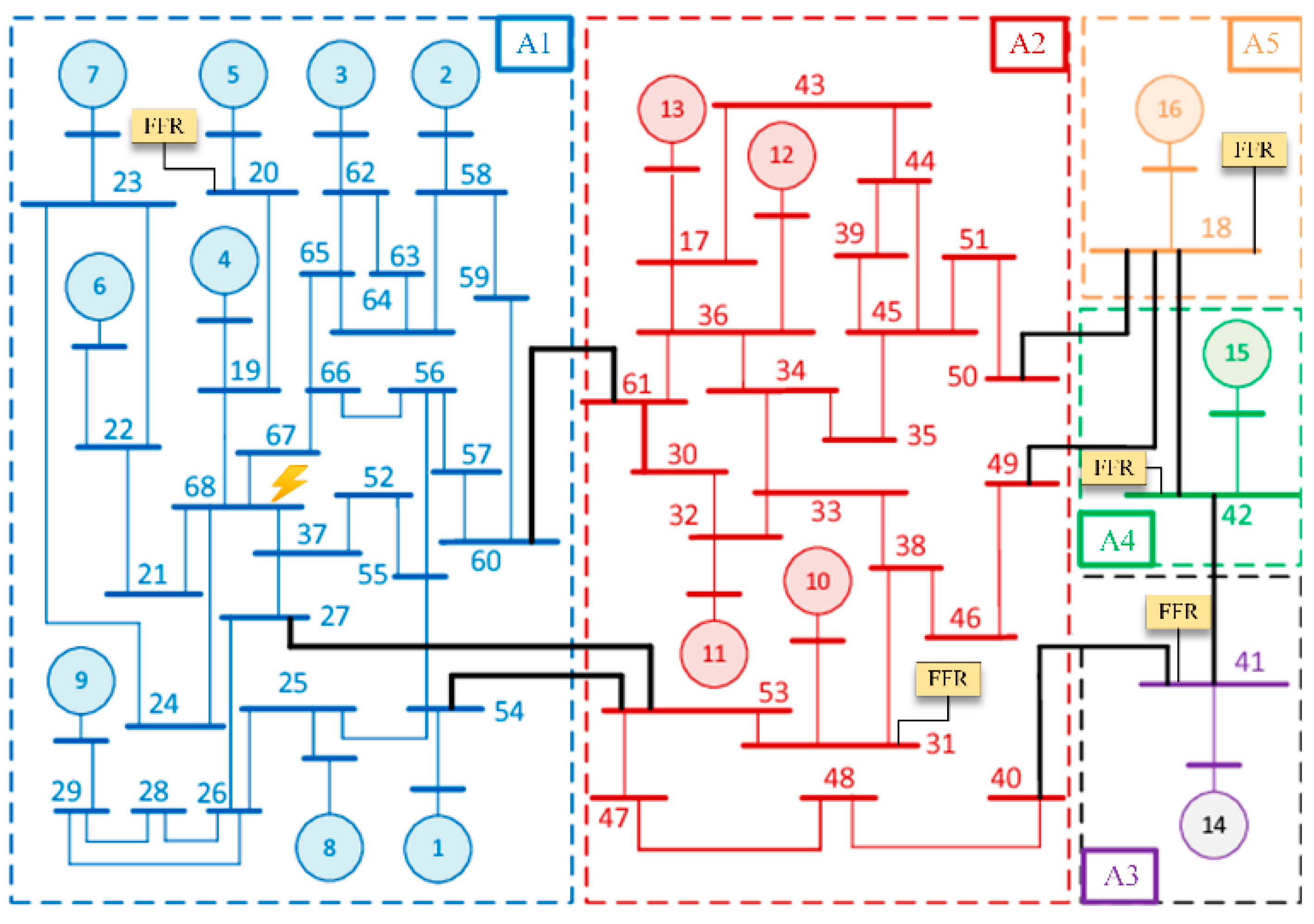
4.2. Simulations on an IEEE 68-Bus System

The IEEE 68-bus system consists of five well-connected areas (A1-A5), and it is a standard test system for dynamic stability analysis [36,37]. Area 1 represents the New England system, area 2 is the system of New York and areas 3, 4 and 5 are represented by an equivalent generator. The state described in [37] was selected as the initial operating state. The load disturbance, which is equivalent to 5% of the total system load, was simulated at bus 68. Two scenarios were considered: the baseline scenario without FFR, and the scenario with three-stage FFR of a capacity of 0.1% of the total system load, implemented in each area. The adopted parameters for the FFR are identical to those in the previous subsection (Table 2), and the FFR providers are connected at buses 20, 31, 41, 42 and 18 (Figure 20).

Figure 21 shows the frequency response after disturbance in Area 1. The solid lines show the frequencies measured at generator buses in the scenario without FFR, whereas the dashed lines show the frequencies at the same buses when FFR is implemented in each area. It can be seen that the generators that belong to the same area have similar frequency behaviors after the disturbance and therefore belong to the same coherent zone. When comparing the generator frequencies for both scenarios, it can be noticed that the frequency deviations are smaller when the FFR is implemented. These results show that the proposed FFR control strategy provides better frequency values compared to the base case.

Figure 22 shows RoCoF values measured at generator buses. The RoCoF is the highest at buses that are close to the disturbance location, and the maximum RoCoF decreases as it goes farther from the disturbance. Moreover, the maximum value of RoCoF is reached later if the bus is farther from the disturbance.

As a direct consequence, the FFR is activated first in the area where the disturbance occurrs, as shown in Figure 23. Moreover, all stages of the FFR are dispatched in Area 1, since the RoCoF values are the highest there. The FFR reserves in Area 2, which are closest to the area where the disturbance occurrs, are activated next. The moments of activation of the FFR in areas 3, 4 and 5 are very similar. Area 3 is electrically more distant to the location of disturbance than areas 4 and 5, and therefore the FFR is activated a little later than it is in areas 4 and 5. In regard to the number of activated FFR stages, in Area 1 where the disturbance happens, all three stages of the FFR are dispatched. In Area 2, which is closer to the disturbance, two stages are dispatched, whereas in areas 3, 4 and 5, only one stage of FFR is dispatched. This confirms that the proposed FFR control strategy considers the locational impact of the disturbance and dispatches more reserves in areas electrically closer to the disturbance. In this way, further propagation of the disturbance through other parts of the system is decreased and slowed down, as shown in Figure 24. The active power flow change on interconnecting lines between Areas 1 and 2 is less when the proposed FFR control strategy is implemented. Therefore, the effects of the disturbance are localized in the area responsible for the generation-load mismatch.

Figure 25 shows the total provision costs when the FFR stages are ranked in merit order based on resource provision costs, compared to the case when there is no prioritization of low-cost resources. The provision cost of the FFR service during the event is reduced when applying low-cost resource prioritization.

5. Conclusions

This paper addresses the frequency stability issue in a low-inertia power system. It proposes a simple design of an FFR control strategy that relies on local measurements of RoCoF and does not need communication infrastructure. As such, it represents a low-cost solution and also avoids time delays due to data transmission. Moreover, by setting a threshold to the measured RoCoF value, the proposed control strategy enables rapid detection of critical frequency events, well before the frequency value drops below the set threshold limit, which consequently enables timely activation of the fast frequency response. The multi-stage principle is introduced as a simple way to deploy reserves proportional to the disturbance and to reduce deployment costs for the FFR ancillary service while respecting the spatial characteristics of the available reserve. The proposed FFR control scheme considers the non-uniform distribution of inertia in the system and the location of the disturbance. By having several stages that are activated at different values of RoCoF, it has been achieved that most reserves are activated closer to the disturbance and in low-inertia parts of the system, which, as a result, minimizes the propagation of the disturbance’s impact on system stability. Furthermore, the novelty of the proposed solutions lies in the fact that this control strategy can rank different kinds of FFR resources based on location and performance and can prioritize the use of low-cost reserves in the case of less severe disturbances. In this way, the economic aspect is also included. Basic insight into the spatial activation of fast frequency control after a disturbance is obtained by simulations on a simple three-area system. The simulations confirm that the implemented FFR control strategy considers the heterogeneity of power system inertia and locational impact of the disturbance, and it dispatches more reserves in areas with low inertia that are electrically closer to the disturbance. Simulations on the IEEE 68-bus system confirm the applicability of the proposed control strategy and verify that the implemented FFR decreases and slows down further propagation of the disturbance through other parts of the system.

6. Future Work

Future work will include the validation of the proposed control strategy using a real-time HIL platform and different FFR resources. Moreover, a detailed method for determining threshold levels of multi-stage FFR activation will be developed, as well as a comprehensive calculation of the amount and number of stages of FFR reserves in different areas. These analyses require detailed system data and a list of potential outages and should be conducted with day-ahead scheduling and reserve planning. Furthermore, an assessment of the locational impact of FFR reserves based on contributions to frequency stability will be also investigated in future research. A method to valorize fast frequency support procurement by different FFR resources will be proposed as a result of these analyses.

References

1. Federico, M.; Florian, D.; Gabriela, H.; David, J.H.; Gregor, V. Foundations and challenges of low-inertia systems (Invited Paper). In Proceedings of the 20th Power Systems Computation Conference (PSCC 2018), Dublin, Ireland, 11–15 June 2018; pp. 1–25. [Google Scholar]
2. Jingyang, F.; Hongchang, L.; Yi, T.; Frede, B. On the inertia of future more-electronics power systems. IEEE J. Emerg. Sel. Top. Power Electron. 2019, 7, 2130–2146. [Google Scholar]
3. Adrees, A.; Milanović, J.V.; Mancarella, P. Effect of inertia heterogeneity on frequency dynamics of low-inertia power systems. IET Gener. Transm. Distrib. 2019, 14, 2019. [Google Scholar] [CrossRef]
4. Wilson, D.; Yu, J.; Al-Ashwal, N.; Heimisson, B.; Terzija, V. Measuring effective area inertia to determine fast-acting frequency response requirements. Int. J. Electr. Power Energy Syst. 2019, 113, 1–8. [Google Scholar] [CrossRef]
5. EirGrid/SONI, Ensuring a Secure, Reliable and Efficient Power System in a Changing Environment, June 2011. Available online: http://www.eirgridgroup.com/site-files/library/EirGrid/Ensuring-a-Secure-Reliable-and-Efficient-Power-System-Report.pdf (accessed on 10 January 2022).
6. National Grid ESO, The Enhanced Frequency Control Capability (EFCC) Project Closing down Report, April 2019. Available online: https://www.nationalgrideso.com/document/144566/download (accessed on 10 January 2022).
7. Australian Energy Market Operator, Future Power System Security Program—Progress Report, August 2016. Available online: https://www.aemo.com.au/Electricity/National-Electricity-Market-NEM/Security-and-reliability/-/media/823E457AEA5E43BE83DDD56767126BF2.ashx (accessed on 10 January 2022).
8. Hong, Q.; Khan, M.A.U.; Henderson, C.; Egea-Àlvarez, A.; Tzelepis, D.; Booth, C. Addressing frequency control challenges in future low-inertia power systems: A great britain perspective. Engineering 2021, 7, 1057–1063. [Google Scholar] [CrossRef]
9. O’Sullivan, J.; Rogers, A.; Flynn, D.; Smith, P.; Mullane, A.; O’Malley, M. Studying the maximum instantaneous non-synchronous generation in an Island system-frequency stability challenges in Ireland. IEEE Trans. Power Syst. 2014, 29, 2943–2951. [Google Scholar] [CrossRef] [Green Version]
10. EirGrid/SONI, All Island TSO Facilitation of Renewables Studies, Jun 2010. Available online: http://www.eirgridgroup.com/site-files/library/EirGrid/Facilitation-of-Renewables-Report.pdf (accessed on 10 January 2022).
11. Australian Energy Market Operator, Power System Security Guideline, January 2022. Available online: https://aemo.com.au/-/media/files/electricity/nem/security_and_reliability/power_system_ops/procedures/so_op_3715-power-system-security-guidelines.pdf?la=en (accessed on 10 February 2022).
12. Ulbig, A.; Borsche, T.S.; Andersson, G. Impact of low rotational inertia on power system stability and operation. IFAC Proc. Vol. 2014, 47, 7290–7297. [Google Scholar] [CrossRef] [Green Version]
13. Nesje, B. The Need for Inertia in the Nordic Power System. Master’s Thesis, NTNU, Trondheim, Norway, 2015. [Google Scholar]
14. Mir, A.S.; Senroy, N. Intelligently controlled flywheel storage for enhanced dynamic performance. IEEE Trans. Sustain. Energy 2019, 10, 2163–2173. [Google Scholar] [CrossRef]
15. Nanou, S.I.; Papakonstantinou, A.G.; Papathanassiou, S.A. A generic model of two-stage grid-connected PV systems with primary frequency response and inertia emulation. Electr. Power Syst. Res. 2015, 127, 186–196. [Google Scholar] [CrossRef]
16. Fu, Y.; Zhang, X.; Hei, Y.; Wang, H. Active participation of variable speed wind turbine in inertial and primary frequency regulations. Electr. Power Syst. Res. 2017, 147, 174–184. [Google Scholar] [CrossRef]
17. Rakhshani, E.; Remon, D.; Cantarellas, A.M.; Garcia, J.M.; Rodriguez, P. Modeling and sensitivity analyses of VSP based virtual inertia controller in HVDC links of interconnected power systems. Electr. Power Syst. Res. 2016, 141, 246–263. [Google Scholar] [CrossRef]
18. Muhssin, M.T.; Cipcigan, L.M.; Obaid, Z.A.; L-Ansari, W.F.A. A novel adaptive deadbeat-based control for load frequency control of low inertia system in interconnected zones north and south of Scotland. Int. J. Electr. Power Energy Syst. 2017, 89, 52–61. [Google Scholar] [CrossRef]
19. Karbouj, H.; Rather, Z.H.; Flynn, D.; Qazi, H.W. Non-synchronous fast frequency reserves in renewable energy integrated power systems: A critical review. Int. J. Electr. Power Energy Syst. 2019, 106, 488–501. [Google Scholar] [CrossRef]
20. Zecchino, A.; Prostejovsky, A.M.; Ziras, C.; Marinelli, M. Large-scale provision of frequency control via V2G: The Bornholm power system case. Electr. Power Syst. Res. 2019, 170, 25–34. [Google Scholar] [CrossRef]
21. Asvapoositkul, S.; Fradley, J.; Preece, R. Incorporation of active power ancillary services into VSC-HVDC connected energy sources. Electr. Power Syst. Res. 2020, 189, 106769. [Google Scholar] [CrossRef]
22. Hong, Q. Fast frequency response for effective frequency control in power systems with low inertia. J. Eng. 2019, 2019, 1696–1702. [Google Scholar] [CrossRef]
23. Eriksson, R.; Modig, N.; Elkington, K. Synthetic inertia versus fast frequency response: A definition. IET Renew. Power Gener. 2018, 12, 507–514. [Google Scholar] [CrossRef]
24. Zhu, J.; Booth, C.D.; Adam, G.P.; Roscoe, A.J.; Bright, C.G. Inertia emulation control strategy for VSC-HVDC transmission system. IEEE Trans. Power Syst. 2013, 28, 1277–1287. [Google Scholar] [CrossRef] [Green Version]
25. Chakravorty, D.; Chaudhuri, B.; Hui, S.Y.R. Rapid Frequency Response from Smart Loads in Great Britain Power System. IEEE Trans. Smart Grid 2017, 8, 2160–2169. [Google Scholar] [CrossRef] [Green Version]
26. Ortega, Á.; Milano, F. Combined frequency and RoCoF control of converter-interfaced energy storage systems. IFAC-PapersOnLine 2019, 52, 240–245. [Google Scholar] [CrossRef]
27. EirGrid, S. DS3 Programme Operational Capability Outlook 2016. 2015. Available online: https://www.eirgridgroup.com/site-files/library/EirGrid/DS3-Operational-Capability-Outlook-2016.pdf) (accessed on 10 January 2022).
28. Pusceddu, E.; Zakeri, B.; Gissey, G.C. Synergies between energy arbitrage and fast frequency response for battery energy storage systems. Appl. Energy 2021, 283, 116274. [Google Scholar] [CrossRef]
29. Bao, P.; Zhang, W.; Cheng, D.; Liu, M. Hierarchical control of aluminum smelter loads for primary frequency support considering control cost. Int. J. Electr. Power Energy Syst. 2020, 122, 106202. [Google Scholar] [CrossRef]
30. Papadogiannis, K.A.; Hatziargyriou, N.D. Optimal Allocation of Primary Reserve Services in Energy Markets. IEEE Trans. Power Syst. 2004, 19, 652–659. [Google Scholar] [CrossRef]
31. Hao, L.; Ji, J.; Xie, D.; Wang, H.; Li, W.; Asaah, P. Scenario-based unit commitment optimization for power system with large-scale wind power participating in primary frequency regulation. J. Mod. Power Syst. Clean Energy 2020, 8, 1259–1267. [Google Scholar] [CrossRef]
32. Hong, Q. Design and validation of a wide area monitoring and control system for fast frequency response. IEEE Trans. Smart Grid 2020, 11, 3394–3404. [Google Scholar] [CrossRef] [Green Version]
33. Ćalović, M.S. Advanced automatic generation control with automatic compensation of tie-line losses. Electr. Power Compon. Syst. 2012, 40, 807–828. [Google Scholar] [CrossRef]
34. Ariff, M.A.M.; Pal, B.C. Coherency identification in interconnected power system—An independent component analysis approach. IEEE Trans. Power Syst. 2013, 28, 1747–1755. [Google Scholar] [CrossRef] [Green Version]
35. Anderson, P.M.; Mirheydar, M. A low-order system frequency response model. IEEE Trans. Power Syst. 1990, 5, 720–729. [Google Scholar] [CrossRef] [Green Version]
36. Canizares, C. Benchmark Systems for Small-Signal Stability Analysis and Control; Technical Report; IEEE Power and Energy Society: Manhattan, NY, USA, 1 August 2015. [Google Scholar]
37. Singh, A.K.; Pal, B.C. IEEE PES Task Force on Benchmark Systems for Stability Controls Report on the 68-Bus, 16-Machine, 5-Area System; Technical Report; IEEE PES Task Force on Benchmark Systems for Stability Controls: Manhattan, NY, USA, 3 December 2013. [Google Scholar]
Figure 1. The maximum values of RoCoF in areas depending on inertia distribution.
Electronics 11 01776 g001
Figure 2. The maximum values of RoCoF in areas depending on area distance.
Electronics 11 01776 g002
Figure 3. The frequency of inter-area oscillations depending on inertia distribution.
Electronics 11 01776 g003
Figure 4. The frequency of inter-area oscillations depending on the synchronizing power coefficient.
Electronics 11 01776 g004
Figure 5. The value of RoCoF in area 1 for different frequencies of inter-area oscillations.
Electronics 11 01776 g005
Figure 6. The value of RoCoF in area 2 for different frequencies of inter-area oscillations.
Electronics 11 01776 g006
Figure 7. Overview of FFR control scheme and the diagram flow of the novel approach implementation.
Electronics 11 01776 g007
Figure 8. Representation of the transmission network divided into coherency areas.
Electronics 11 01776 g008
Figure 9. The provision of FFR in one stage.
Electronics 11 01776 g009
Figure 10. Timeline and cost associated with FFR service.
Electronics 11 01776 g010
Figure 11. Dispatch of FFR resources based on provision cost.
Electronics 11 01776 g011
Figure 12. Three-area test system.
Electronics 11 01776 g012
Figure 13. Three-area test system response in the case of a disturbance in Area2—Strong grid—Case 1.1.
Electronics 11 01776 g013
Figure 14. Three-area test system response in the case of a disturbance in Area2—Weak grid—Case 1.2.
Electronics 11 01776 g014
Figure 15. Three-area test system response in the case of a disturbance in Area2—Different line lengths—Case 1.3.
Electronics 11 01776 g015
Figure 16. Three-area test system response in the case of a disturbance in a low-inertia area—Case 2.1.
Electronics 11 01776 g016
Figure 17. Three-area test system response in the case of a disturbance in the high-inertia area—Case 2.2.
Electronics 11 01776 g017
Figure 18. FFR deployment for different location of the disturbance.
Electronics 11 01776 g018
Figure 19. Provision costs of FFR service.
Electronics 11 01776 g019
Figure 20. IEEE 68-bus system.
Electronics 11 01776 g020
Figure 21. Frequencies at generator buses after disturbance in Area 1.
Electronics 11 01776 g021
Figure 22. The RoCoF at generator buses after disturbance in Area 1.
Electronics 11 01776 g022
Figure 23. FFR in different areas.
Electronics 11 01776 g023
Figure 24. Active power flow on lines connecting Area 1 and Area 2.
Electronics 11 01776 g024
Figure 25. Provision costs of FFR service for the IEEE 68.
Electronics 11 01776 g025