Article

Research on Orbital Angular Momentum Multiplexing Communication System Based on Neural Network Inversion of Phase

1
Periodical Agency of Chongqing University of Technology, Chongqing University of Technology, Chongqing 400054, China
2
School of electrical and Electronic Engineering, Chongqing University of Technology, Chongqing 400054, China
*
Author to whom correspondence should be addressed.
Electronics 2022, 11(10), 1592; https://doi.org/10.3390/electronics11101592
Submission received: 20 April 2022 / Revised: 12 May 2022 / Accepted: 13 May 2022 / Published: 17 May 2022
(This article belongs to the Special Issue Mechatronic Control Engineering)

Abstract

:
An adaptive optical wavefront recovery method based on a residual attention network is proposed for the degradation of an Orbital Angular Momentum multiplexing communication system performance caused by atmospheric turbulence in free-space optical communication. To prevent the degeneration phenomenon of neural networks, the residual network is used as the backbone network, and a multi-scale residual hybrid attention network is constructed. Distributed feature extraction by convolutional kernels at different scales is used to enhance the network’s ability to represent light intensity image features. The attention mechanism is used to improve the recognition rate of the network for broken light spot features. The network loss function is designed by combining realistic evaluation indexes so as to obtain Zernike coefficients that match the actual wavefront aberration. Simulation experiments are carried out for different atmospheric turbulence intensity conditions, and the results show that the residual attention network can reconstruct the turbulent phase quickly and accurately. The peaks to valleys of the recovered residual aberrations were between 0.1 and 0.3 rad, and the root means square was between 0.02 and 0.12 rad. The results obtained by the residual attention network are better than those of the conventional network at different SNRs.

1. Introduction

Orbital Angular Momentum (OAM) has become an object of research as one of the means to improve the transmission efficiency of optical communication [1]. Recently, stable data transmission at the Tbit/s level has been achieved in the laboratory by multiplexing OAM beams [2]. OAM multiplexed communication can be combined with polarization multiplexing and wavelength division multiplexing to enhance the transmission rate [3]. The transmission rate can be further improved by combining OAM multiplexing with Multiple Input Multiple Output (MIMO) spatial multiplexing techniques [4]. In addition, for OAM multiplexing-based Free Space Optical Communications (FSO) systems, MIMO equalization techniques can be utilized. A constant-mode blind equalization algorithm is used to improve the BER degradation in OAM multiplexing systems due to atmospheric turbulence [5]. It can also be combined with optimal mode selection strategies to ensure the communication quality at high-speed communication [6]. However, in FSO systems, the atmospheric refractive index variations due to atmospheric turbulence cause random amplitude undulations as well as phase distortions in the atmospherically transmitted laser beam, resulting in degradation of the performance of the FSO system [7].
Adaptive Optics (AO) technology can achieve an improved performance of communication systems by correcting the dynamic wavefront aberrations of the beam [8]. In AO, wavefront-free detection AO systems can directly use the light intensity information to design control algorithms that generate the control signals required by the wavefront corrector, i.e., wavefront reconstruction based on the aberrated light intensity image [9]. Classical wavefront reconstruction methods for wavefront-free detection include the Gerchberg–Saxton (GS) phase recovery algorithm, stochastic parallel gradient descent algorithm, simulated annealing algorithm, and genetic algorithm [10], which mostly need to be solved by iterative computation and are difficult to achieve real-time wavefront reconstruction.
Recently, deep learning techniques have been widely used in AO. Deep learning-based wavefront-free detection aims to use the light intensity image captured by the charge coupled device (CCD) camera as the input of a neural network and the wavefront aberration or Zernike coefficient as the output; then, the output is transformed into the control signal, and finally, the deformation mirror is controlled to achieve wavefront correction. Paine et al. [11] applied a deep learning approach to the point expansion function to achieve wavefront reconstruction. Tian et al. [12] recovered the wavefront based on a deep neural network model to address the problem of too many iterations of existing search algorithms. These studies showed the effectiveness of deep neural network models, and to reduce the computational complexity, Nishizaki et al. [13] estimated wavefront Zernike coefficients directly from a single light intensity image by using a convolutional neural network model and improved the network estimation performance by preprocessing. Zhai et al. [14] also used a convolutional neural network model to reduce the computation time. Ma et al. [15], inspired by the phase difference approach, proposed to use the light intensity maps in the focal and out-of-focus planes as the input to the neural network and output of the wavefront Zernike coefficients. Ma et al. [16] also explored the effect of the consistency of the training data on the wavefront recovery performance. Wu et al. [17] also used a convolutional neural network to establish a mapping of the real image to its Zernike coefficients based on the idea of phase difference. Zhang et al. [18] used residual networks to obtain wavefront Zernike coefficients and verified the robustness of deep residual networks.
The above literature shows that deep convolutional neural networks have shown better performance than traditional wavefront detection algorithms in wavefront-free detection AO systems, but they still suffer from inadequate perception and representation of light spot features. As the number of network layers deepens, gradient disappearance, explosion and overfitting are prone to occur, making it difficult to accomplish real-time accurate reconstruction tasks. Too many pooling operations can also lead to the loss of small target information, resulting in excessive reconstruction errors.

2. Vortex Beam Atmospheric Transport Model

The schematic diagram of the OAM state multiplexed communication system with wavefront correction is shown in Figure 1. The system starts with n path independent messages transmitted using binary signals, and then, it passes through an optical modulator for baseband signal modulation, modulating each user’s message onto a Gaussian optical carrier and then loading the OAM mode using different OAM mode converters. The next n path OAM state signals are multiplexed by optical intensity superposition and distorted by optical intensity distortion after atmospheric turbulence. To reduce the effects of mode crosstalk and turbulence, wavefront correction techniques are introduced to improve the received optical quality. Afterward, the OAM light is transformed back to Gaussian light by OAM state demultiplexing and inverse converters, and finally, the signal is demodulated into a binary signal by an optical demodulator.
In free-space optical communication, the vortex beam has a continuous spiral wavefront compared to an ordinary beam, and the phase has uncertainty in the direction of beam propagation, where the phase singularity is. The Laguerre–Gauss (LG) beam in the vortex beam is a representative beam, and its light field expression in free space is shown in the following equation [19].
u p l ( r , φ , z ) = 2 p ! π ( p + | l | ) ! 1 w ( z ) [ 2 w ( z ) ] | l | × L p | l | [ 2 r 2 w 2 ( z ) ] exp [ r 2 w 2 ( z ) ] × exp ( i l φ ) exp [ i k r 2 z 2 ( z 2 + z 0 2 ) ] × exp [ i ( 2 p + | l | + 1 ) arctan ( z z 0 ) ]
where p denotes the radial index of the LG beam; r is the radial distance from the spatial point to the transmission axis; φ is the azimuth angle; w ( z ) = w 0 1 + ( z / z 0 ) 2 , w 0 is the beam waist radius; L p | l | is the Laguerre polynomial, l is the topological charge of the vortex beam, which can be taken as an integer; k = 2 π / λ is the wavenumber; and z 0 = k w 0 / λ is the Rayleigh distance.
When the light wave passes through multiple phase screens, only the phase changes while the amplitude remains the same. Under the Rytov approximation, the expression for the optical field at a transmission distance of Δ z can be obtained, as shown in the following equation [20].
u ( r , φ , z i + 1 ) = 1 { { u ( r , φ , z i ) exp [ i ϕ ( r , z i ) ] } exp [ i ( k x 2 + k y 2 ) Δ z 2 k ] }
where 1 and denote the Fourier inverse transform and Fourier transform, respectively; ϕ ( r , z i ) denotes the atmospheric turbulence phase screen function; k x and k y denote the number of spatial waves in x and y directions, respectively, and k = k x 2 + k y 2 + k z 2 .
Therefore, only the phase screen model of atmospheric turbulence needs to be simulated to calculate the magnitude of the optical field at the receiving end. In this paper, the Zernike polynomial defined by Noll is chosen to model the turbulent phase screen ϕ ( r ) , which can be expressed by the following equation.
ϕ ( r ) = i a i Z i
{ Z e v e n i = n + 1 R n m ( r ) 2 cos ( m θ ) , m 0 Z o d d i = n + 1 R n m ( r ) 2 sin ( m θ ) , m 0 Z i = n + 1 R n 0 ( r ) , m = 0
R n m ( r ) = s = 0 ( n m ) / 2 ( 1 ) s ( n s ) ! s ! [ ( n + m ) / 2 s ] ! [ ( n m ) / 2 s ] ! r n 2 s
where r and θ are polar coordinates. n and m are the radial and angular steps, respectively; they are always integers and satisfy the following condition: m n , n | m | = e v e n .
The first term of the Zernike polynomial represents the translation, which has no effect on the image imaging quality. Higher-order polynomials, which can represent higher-frequency components, are therefore disregarded in this paper, and a polynomial of order 36 is selected to generate a realistic atmospheric turbulence phase screen.
Denoting the ith input signal as x i ( t ) , each signal will piggyback on the corresponding OAM mode, so the output signal of each OAM state is denoted as X i T x = x i ( t ) u i ( r , φ , z ) . The n-way signal multiplexing yields the following equation.
X m u x T x = i = 1 n x i ( t ) u i ( r , φ , z )
After atmospheric transmission, assuming that the mode crosstalk and noise are independent of each other during transmission, the received signal can be expressed as the following equation.
Y m u x T x = i = 1 n x i ( t ) u i ( r , φ , z ) + n ( t )
where u i = u i × exp ( j ϕ ) denotes the beam after atmospheric turbulence.
In demultiplexing, the interference of external factors destroys the orthogonality between the vortex beams and causes mode crosstalk; the information of its kth path can be expressed by the following equation.
y k ( t ) = Y m u x T x , u k ( r , φ , z ) = i = 1 n x i ( t ) u i ( r , φ , z ) u i * ( r , φ , z ) r d r d φ + n ( t ) u i * ( r , φ , z ) r d r d φ = x k ( t ) u i ( r , φ , z ) u i * ( r , φ , z ) r d r d φ + i = 1 , i k n x i ( t ) u i ( r , φ , z ) u i * ( r , φ , z ) r d r d φ + n ( t ) u i * ( r , φ , z ) r d r d φ

3. Residual Hybrid Attention Network Model

3.1. Residual Network Model

Continuously increasing the depth of the network is not only easy to overfit but also very easy to obtain a local optimal solution, and the convolution operation will lead to differences in the extracted features between pixels that are originally connected due to the difference in the perceptual field size, resulting in a large reconstruction aberration. To address the above problems, this paper uses the idea of layer-hopping connection to construct a constant mapping of feature maps, which enables the later layers to learn the residuals of the network and reduce the risk of overfitting. Combined with global contextual information, an attention mechanism is added to establish connections between features and increase the wavefront reconstruction ability of the network. The wavefront reconstruction system based on the residual network is shown in Figure 2.
The backbone network is the ResNet50 model, which first transforms the input light intensity map into a feature image by 7 × 7 downsampling convolution, which is followed by a maximum pooling operation to reduce the parameters of the feature map. The hybrid attention module is then embedded into the ResNet model to fully capture the feature information. Dropout is added to prevent overfitting, and finally, the three-dimensional feature map is mapped to the one-dimensional feature map by the fully connected layer, and the final output is the Zernike coefficient corresponding to the wavefront aberration in the input light intensity map.

3.2. Hybrid Attention Structure

To compensate for the limited sensory field of deep ResNet and the lack of cross-channel interaction, this paper adds a spatial attention (SA) mechanism and channel attention (CA) mechanism to the network, whose main architecture is derived from the dynamic Selective Kernel Neural Networks (SKNet) [21]. The information related to the feature mapping is mainly extracted by convolution operation, and the residual hopping structure is added to reasonably allocate computational resources to the model according to the importance of the input features. By integrating the spatial attention module and the channel attention module, a hybrid attention mechanism model was constructed. The structure is shown in Figure 3.
For spots of different sizes in the light intensity image, the scale of the features varies equally. If convolution kernels of the same size are used, the ability to express the feature information of small spots gradually becomes weaker, leading to an increase in reconstruction aberration error. To address this, this paper uses SKNet, a multi-scale feature extraction network, to enable the model to enhance the representation of shallow features, which facilitates the regression of smaller targets in the network and allows the model to focus more on the targets themselves.
SKNet can be divided into three parts: decomposition, fusion and selection. In the decomposition part, convolutional kernels of different sizes are selected for feature mapping operations. Although the multi-branch structure can tap richer semantic information and enhance the expressiveness of the network, it also increases the difficulty of network training. Therefore, a two-way network structure of 3 × 3 and 5 × 5 size is chosen in this paper, which is represented by the following equation.
U ˜ = f 3 × 3 ( X ) R h × w × C
U ^ = f 5 × 5 ( X ) R h × w × C
where X R h × w × C is the input feature map and f represents the convolution operation so that not only the feature representation of the high and low-frequency parts of the light intensity image can be obtained through the multi-branch structure, but also, too many network branches can be avoided to cause training difficulties in convergence. The 5 × 5 convolution uses the null convolution operation.
In the fusion part, the feature maps are summed by the summation operation control, and then, s is obtained by global average pooling the information carried by each channel of the statistical convolution layer, and finally, feature dimensionality reduction is performed to obtain z . The overall process is shown in the following equation.
U = U ˜ + U ^
s = g p ( U ) = 1 h × w i = 1 h j = 1 w U ( i , j )
z = f c ( s ) = δ ( ( W s ) )
where g p is the global pooling operation, f c is the fully connected operation, δ is the Rectified linear unit (Relu), is the Batch Normalization layer, W s R d × C , d = max ( C / r , L ) denotes the feature dimension after full connection, r is the compression factor, and L denotes the minimum value of d . The global attention module is used to integrate deep and shallow features to alleviate the problem of losing information of smaller spots caused by the low resolution of deep features.
For the selection part, the softmax function is used to calculate the weight distribution of each channel. The calculation is shown in the following equation.
a c = e A c z e A c z + e B c z , b c = e B c z e A c z + e B c z
V = a · U ˜ + b · U ^ , a c + b c = 1
where a and b are soft attention weight matrices for the two channels, respectively.
The amount of high-frequency information is further reduced due to the presence of pooling layers, resulting in a weaker representation of deep features for small targets. In this paper, we introduce a spatial attention mechanism to weight the features of the target region and find the connection between features in the network so that the feature extraction network selectively focuses on the target region containing important information. The final output matrix is calculated as shown below.
V ˜ = σ ( f 5 × 5 ( c [ a v g ; max ] ) )
Y = V · V ˜
where c denotes the splicing operation, σ is the sigmoid activation function. a v g and max denote the average pooling operation and the maximum pooling operation performed along the channel axis, respectively. Unlike channel attention, spatial attention can distinguish high and low-frequency information, which is complementary to channel attention [22], and feature maps optimized for spatial information can effectively express the feature similarity between pixel points, and spatial attention can be a good way to obtain contextual semantic information.

3.3. Loss Function

To make the reconstruction of Zernike coefficient of wavefront aberration more reasonable, this paper combines the commonly used wavefront evaluation metrics to improve the loss function of the network. The commonly used AO system evaluation metrics are peak to valley (PV) and root mean square (RMS); PV is used to represent the difference between the highest and lowest points of the wavefront, and RMS characterizes the deviation of the measured beam wavefront compared to the ideal wavefront [23], and its formula is shown below.
P V = max ( Δ ϕ ( ρ , θ ) ) min ( Δ ϕ ( ρ , θ ) )
Y = V · V ˜
where Δ ϕ is the wavefront aberration and Δ ϕ ¯ is its mean value. ρ and θ are the polar coordinates of the optical pupil surface.
It can be seen from the equation that the PV value does not reflect the wavefront information comprehensively, while the RMS value focuses more on the overall wavefront information, and combining the two can represent the wavefront situation more accurately. Therefore, the loss function of the combined MSE is shown below.
M S E = 1 N i = 0 N ( z a c t i z p r e i ) 2
= λ M S E M S E + λ P V P V + λ R M S R M S
where z a c t and z p r e are the actual and estimated Zernike coefficients, respectively, with length N , λ is the weight of each loss, is the weighted sum of each loss function, and the reduction in the loss function represents the improvement of the reconstruction accuracy.

4. Deep Learning-Based Wavefront Recovery Simulation Experiments

To verify the effectiveness of the residual attention network proposed in this paper, experimental simulations of vortex beam transmission are carried out to develop experimental simulations of wavefront recovery at different turbulence intensities. The vortex beam undergoes phase distortion after passing through atmospheric turbulence, as shown by Equation (6). The Zernike coefficient is not statistically independent but follows a Kolmogorov distribution, and its magnitude is related to the D / r 0 ratio, where D is the system aperture diameter and r 0 is the atmospheric coherence length. For systems with reception apertures up to 1 m [24], D / r 0 = 2 can represent weak turbulence, D / r 0 = 10 can represent medium turbulence, and D / r 0 = 20 can represent strong turbulence. The rest of the parameters [25] are set as shown in Table 1.
In addition, to make the experiment more reasonable, a range of ratios was set at an interval of 2 to D / r 0 = 2 ~ 20 . Each ratio generates 5000 sets of random Zernike coefficients and corresponding light intensity maps as training data. The ratio of the training set, validation set and test set is 8:1:1, the size of the training image is adjusted to 224 × 224 pixels, and the output of the network is 36 Zernike coefficients. To make the experimental comparison clearer, the next test will also generate the corresponding wavefront phase from the output Zernike coefficients for comparison and test the network accuracy from the residuals between the predicted phase and the true phase. The turbulence phase screen and light intensity distribution map shown in Figure 4 can be generated from Equation (3) and the parameters in Table 1. In Figure 4a–c, the phase screens of atmospheric turbulence simulated by Zernike coefficients at different turbulence intensities are represented in degrees, and the PV and RMS values in rad are shown in the figure, with larger values representing larger phase screen undulations and worse atmospheric conditions.
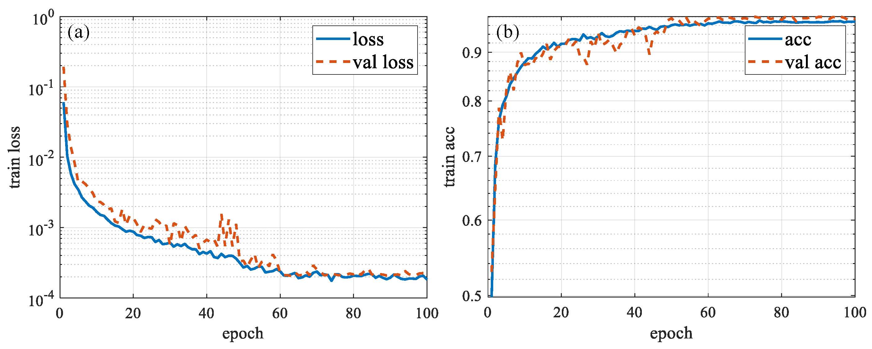
The experimental simulation environment uses the Keras deep learning library in Python language, and the offline training epoch is set to 100, and each batch size is set to 50. The adaptive learning rate Adam algorithm is used to set the initial learning rate to 0.001, and the learning rate decreases to 0.0001 when the network accuracy is not increased within 10 batches. The dropout layer is used in the fully connected layer to prevent network overfitting, and the tanh function is used as the network activation function. Through comprehensive evaluation of experiments, the weights of each part of the loss function in this paper are set to λ M S E = 1 , λ P V = 0.5 , λ R M S = 0 . 5 . The value of the loss function and the size of the accuracy rate in the training process are shown in Figure 5.
In Figure 5, the loss function in Figure 5a decreases as the number of iterations increases, and the accuracy rate in Figure 5b gradually increases, and finally, the overall accuracy rate can reach about 96%. The variation of loss value (val_loss) and accuracy value (val_acc) in the validation set is close to that in the training set, which indicates that the network structure is reasonably designed and there is no overfitting phenomenon, and its accuracy rate can reach about 97%.
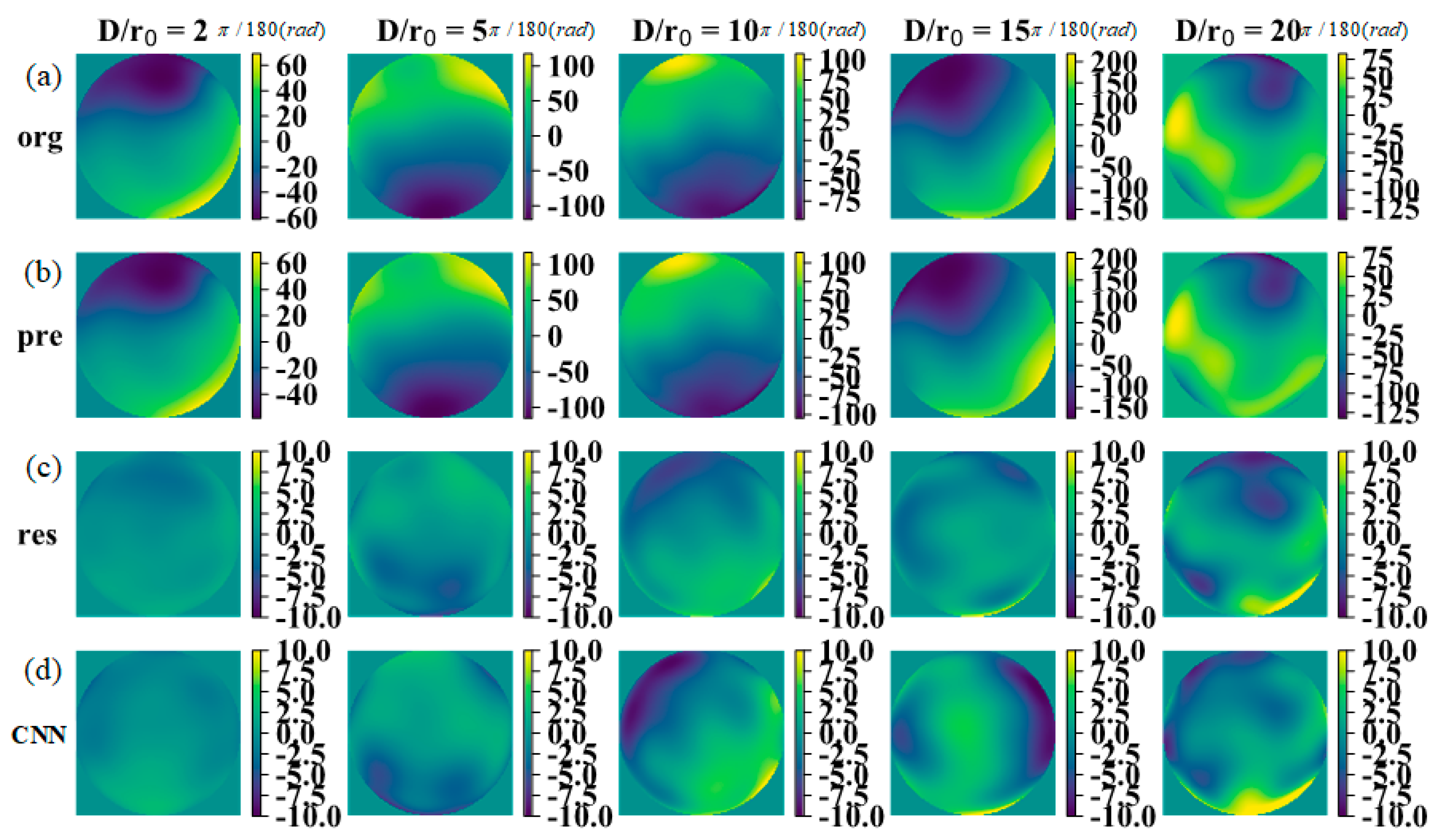
To verify the effectiveness and robustness of the residual attention network model, five sets of Zernike coefficients were randomly generated in the experiment at different turbulence intensities, and the corresponding phase screens were generated as shown in Figure 6a. The Zernike coefficients are predicted by the hybrid attention network model proposed in this paper, and the estimated results and their residual phases are shown in Figure 6b,c, and the results of the literature using CNN are shown in Figure 6d. It can be seen that the residuals predicted by the residual attention network model proposed in this paper have the smallest residuals, and the results predicted by the model using only convolutional neural networks are not accurate enough. The PV and RMS values of the residual phase are shown in Table 2. The aberrated phase residuals predicted by the method in this paper have smaller values and can obtain a more realistic phase screen compared to the previous work. Therefore, it can be seen from Figure 6 and Table 2 that the hybrid attention network has a good reconstruction effect at different turbulence intensities, and the recovered phase screen is similar to the actual phase screen. Figure 7 shows the comparison between the predicted Zernike coefficients and the actual coefficients for five different turbulence intensities, and it can be seen that the predicted results of the method in this paper are closer to the actual coefficients.
After reconstructing the wavefront based on the predicted Zernike coefficients, the correction of the turbulent phase can be achieved by loading an inverse phase wavefront to the distorted beam. To verify the effectiveness of the inverse phase of the residual attention network in the OAM multiplexed communication system, the topological charge of the fixed transmission beam is 1, −2, 3, and −5, the signal-to-noise ratio is set to 10, the modulation is quadratic phase-shift keying, and other conditions remain unchanged, and the experimental simulation is carried out under different turbulence intensities, the results of which are shown in Figure 8. It can be seen that the system BER increases as the turbulence intensity becomes stronger. Compared with the CNN network model, the system with the lowest BER after correction using the model in this paper, the system performance is not improved much after using the Gerchberg–Saxton phase recovery algorithm. The system without the phase correction algorithm has the highest BER, which is indicated by none in the figure, and it can be seen that the BER of the uncorrected signal hardly exceeds the Forward Error Correction (FEC) limit.
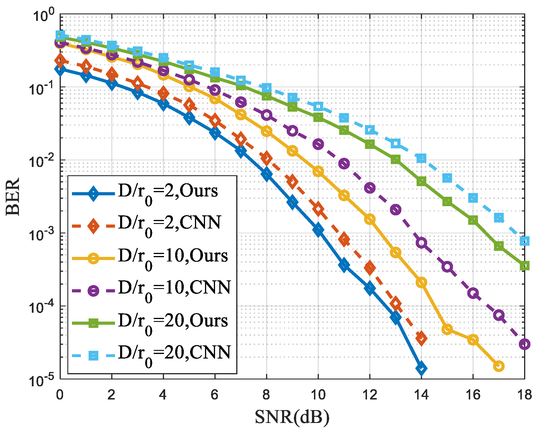
To verify the robustness of the residual attention network model, experimental simulations were performed at different signal-to-noise ratios and turbulence intensities, and the results obtained are shown in Figure 9. As can be seen from the figure, the BER increases as the turbulence intensity becomes stronger, but better results than the CNN network can be obtained using the model proposed in this paper at either turbulence intensity. At a BER of 10−3, this model has a performance gain of about 1 dB compared to the CNN model. As can be seen from the figure, the signal corrected by the residual attention model has better BER performance and can reach the FEC limit faster than the CNN model.
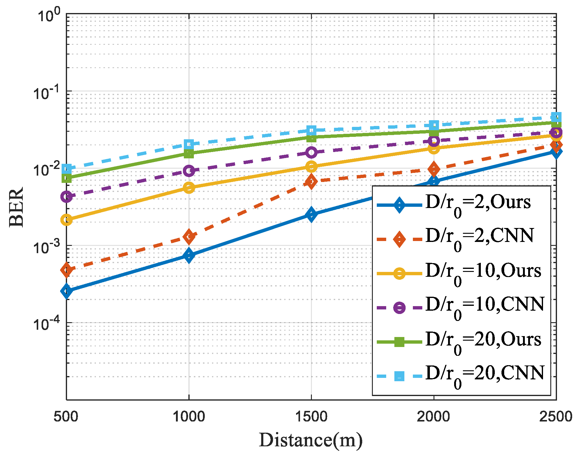
Distance is one of the key factors affecting the performance of optical communication systems, and the BER of the system grows with the increase in transmission distance. In the experiment, the same simulation conditions were set with a signal-to-noise ratio of 10 and no other conditions were varied, and the comparison was performed at different distances and turbulence intensities, and the results obtained are shown in Figure 10. From the figure, it can be seen that the turbulence effect becomes larger and the system performance becomes worse as the distance increases. At different turbulence intensities, the system corrected using the model in this paper has the lowest BER, which indicates the robustness of the model. As seen in the figure, the residual attention model can reach the FEC limit faster at an SNR of 10.
To verify the effectiveness of the hybrid attention structure proposed in this paper, several different models were trained in the experiments, including the base backbone network ResNet50, the network with CA added, the network with SA added, and the network with the hybrid attention structure added, and the accuracy and running time comparison results were obtained, as shown in Table 3.
Table 3 shows that the network with the added attention mechanism has the highest accuracy in reconstructing the Zernike coefficients and the hybrid attention structure has a higher accuracy of 97.3% compared to the single attention structure. In terms of the running time, the average value was taken after testing 1000 times, and it can be seen from the table that the computation time of the added attention network is all below 10 ms, which can meet the requirement of real-time wavefront correction, and the running time can continue to decrease with the increase in hardware performance. The running time of the hybrid attention structure is slightly longer than that of ResNet50, but the performance of the residual attention network proposed in this paper is the best after comprehensive accuracy is evaluated.

5. Conclusions

In this paper, we propose an inverse wavefront phase of the AO system combined with a residual attention network to achieve effective wavefront correction and thus reduce the system BER by addressing the problem of vortex beam distortion caused by atmospheric turbulence, which leads to the degradation of FSO communication quality. The trained model establishes an accurate mapping between the first 36th-order Zernike coefficients and the aberrated light intensity distribution. Experimental simulations were performed under different turbulence conditions, and the obtained wavefront residuals PV and RMS values showed an improvement over previous studies, indicating the strong robustness of the network. At a BER of 10−3, the residual attention network has a performance gain of about 1 dB compared to the CNN network. In the case of D / r 0 = 2 , PV = 0.094 rad, RMS = 0.018 rad; in the case of D / r 0 = 10 , PV = 0.236 rad, RMS = 0.085 rad; in the case of D / r 0 = 20 , PV = 0.335 rad, RMS = 0.122 rad. The predicted Zernike coefficients are similar to the actual coefficients, and the phases reconstructed by the coefficients are highly similar to the actual phases. The effectiveness of the hybrid attention network in the reconstructed wavefront phase task is then verified, with the highest accuracy with less increase in time complexity. The high accuracy, real-time performance, and flexibility of the residual attention network provide the practical application of deep learning in AO systems.

Author Contributions

Conceptualization, Y.C. and Z.Z.; methodology, Y.C. and Z.Z.; software, H.Q. and X.P.; validation Y.C., Z.Z., X.P., H.Q. and Y.W.; formal analysis, Z.Z.; investigation X.P.; resources, H.Q.; data curation, X.P.; writing—original draft preparation, Z.Z.; writing—review and editing, Z.Z.; project administration, Y.C.; funding acquisition, Y.C. All authors have read and agreed to the published version of the manuscript.

Funding

Project supported by the Education Commission Foundation of Chongqing (Grant No. KJ1500934), Science and technology project of Chongqing Education Commission (Grant No. KJ1709205), the graduate scientific research innovation project of Chongqing (Grant No. CYS18311), the basic and frontier research program of Chongqing (Grant No. cstc2015jcyjA40051), the Science and Technology Program of Chongqing Banan (Grant No. 2019TJ07) Science and Technology Research Youth Project of Chongqing Education Commission (Grant No. KJQN202101124).

Conflicts of Interest

The authors declare no conflict of interest.

References

  1. Zhu, L.; Xin, X.; Chang, H.; Wang, X.; Tian, Q.; Zhang, Q.; Gao, R.; Liu, B. Security enhancement for adaptive optics aided longitudinal orbital angular momentum multiplexed underwater wireless communications. Opt. Express 2022, 30, 9745–9772. [Google Scholar] [CrossRef]
  2. Zhang, J.; Liu, J.; Shen, L.; Zhang, L.; Luo, J.; Liu, J.; Yu, S. Mode-division multiplexed transmission of wavelength-division multiplexing signals over a 100-km single-span orbital angular momentum fiber. Photonics Res. 2020, 8, 1236–1242. [Google Scholar] [CrossRef]
  3. Huang, H.; Xie, G.; Yan, Y.; Ahmed, N.; Ren, Y.; Yue, Y.; Rogawski, D.; Willner, M.J.; Erkmen, B.I.; Birnbaum, K.M.; et al. 100 Tbit/s free-space data link enabled by three-dimensional multiplexing of orbital angular momentum, polarization, and wavelength. Opt. Lett. 2014, 39, 197–200. [Google Scholar] [CrossRef] [Green Version]
  4. Ren, Y.; Wang, Z.; Xie, G.; Li, L.; Cao, Y.; Liu, C.; Liao, P.; Yan, Y.; Ahmed, N.; Zhao, Z.; et al. Free-space optical communications using orbital-angular-momentum multiplexing combined with MIMO-based spatial multiplexing. Opt. Lett. 2015, 40, 4210–4213. [Google Scholar] [CrossRef] [PubMed]
  5. Huang, H.; Cao, Y.; Xie, G.; Ren, Y.; Yan, Y.; Bao, C.; Ahmed, N.; Neifeld, M.A.; Dolinar, S.J.; Willner, A.E. Crosstalk mitigation in a free-space orbital angular momentum multiplexed communication link using 4×4 MIMO equalization. Opt. Lett. 2014, 39, 4360–4363. [Google Scholar] [CrossRef] [PubMed]
  6. Wang, L.; Jiang, F.; Chen, M.-K.; Dou, H.; Gui, G.; Sari, H. Interference Mitigation Based on Optimal Modes Selection Strategy and CMA-MIMO Equalization for OAM-MIMO Communications. IEEE Access 2018, 6, 69850–69859. [Google Scholar] [CrossRef]
  7. Wang, A.; Zhu, L.; Deng, M.; Lu, B.; Guo, X. Experimental demonstration of OAM-based transmitter mode diversity data transmission under atmosphere turbulence. Opt. Express 2021, 29, 13171–13182. [Google Scholar] [CrossRef]
  8. Guo, Q.; Cheng, S.; Ke, X. Experimental Study of Large-amplitude Wavefront Correction in Free-space Coherent Optical Communication. Curr. Opt. Photonics 2021, 5, 627–640. [Google Scholar] [CrossRef]
  9. Yazdani, R.; Hajimahmoodzadeh, M.; Fallah, H. Adaptive phase aberration correction based on imperialist competitive algorithm. Appl. Opt. 2014, 53, 132–140. [Google Scholar] [CrossRef]
  10. Wang, X.; Yu, H.; Huang, Q.; Zhang, Z.; Zhou, Z.; Fu, Z.; Xia, P.; Wang, Y.; Jiang, X.; Yang, J. Polarization-independent fiber-chip grating couplers optimized by the adaptive genetic algorithm. Opt. Lett. 2021, 46, 314–317. [Google Scholar] [CrossRef]
  11. Paine, S.W.; Fienup, J. Machine learning for improved image-based wavefront sensing. Opt. Lett. 2018, 43, 1235–1238. [Google Scholar] [CrossRef] [PubMed]
  12. Tian, Q.; Lu, C.; Liu, B.; Zhu, L.; Pan, X.; Zhang, Q.; Yang, L.; Tian, F.; Xin, X. DNN-based aberration correction in a wavefront sensorless adaptive optics system. Opt. Express 2019, 27, 10765–10776. [Google Scholar] [CrossRef] [PubMed]
  13. Nishizaki, Y.; Valdivia, M.; Horisaki, R.; Kitaguchi, K.; Saito, M.; Tanida, J.; Vera, E. Deep learning wavefront sensing. Opt. Express 2019, 27, 240–251. [Google Scholar] [CrossRef] [PubMed]
  14. Zhai, Y.; Fu, S.; Zhang, J.; Liu, X.; Zhou, H.; Gao, C. Turbulence aberration correction for vector vortex beams using deep neural networks on experimental data. Opt. Express 2020, 28, 7515–7527. [Google Scholar] [CrossRef] [PubMed]
  15. Ma, H.; Liu, H.; Qiao, Y.; Li, X.; Zhang, W. Numerical study of adaptive optics compensation based on Convolutional Neural Networks. Opt. Commun. 2019, 433, 283–289. [Google Scholar] [CrossRef]
  16. Ma, H.; Jiao, J.; Qiao, Y.; Liu, H.; Gao, Y. Wavefront Restoration Method Based on Light Intensity Image Deep Learning. Laser Optoelectron. Prog. 2020, 57, 255–264. [Google Scholar]
  17. Wu, Y.; Guo, Y.; Bao, H.; Rao, C. Sub-Millisecond Phase Retrieval for Phase-Diversity Wavefront Sensor. Sensors 2020, 20, 4877. [Google Scholar] [CrossRef] [PubMed]
  18. Zhang, Y.; He, Y.; Ning, Y.; Sun, Q.; Li, J.; Xu, X. Deep learning method of far-field spot inversion wavefront phase. Infrared Laser Eng. 2021, 50, 278–287. [Google Scholar]
  19. Anguita, J.A.; Neifeld, M.A.; Vasic, B.V. Turbulence-induced channel crosstalk in an orbital angular momentum-multiplexed free-space optical link. Appl. Opt. 2008, 47, 2414–2429. [Google Scholar] [CrossRef]
  20. Zhang, Y.; Wang, P.; Guo, L.; Wang, W.; Tian, H. Performance analysis of an OAM multiplexing-based MIMO FSO system over atmospheric turbulence using space-time coding with channel estimation. Opt. Express 2017, 25, 19995–20011. [Google Scholar] [CrossRef]
  21. Li, X.; Wang, W.; Hu, X.; Yang, J. Selective kernel networks. In Proceedings of the 2019 IEEE/CVF Conference on Computer Vision and Pattern Recognition (CVPR), Long Beach, CA, USA, 15–20 June 2019; pp. 510–519. [Google Scholar] [CrossRef] [Green Version]
  22. Zagoruyko, S.; Komodakis, N. Paying more attention to attention: Improving the performance of convolutional neural networks via attention transfer. In Proceedings of the 5th International Conference on Learning Representations, (ICLR), Toulon, France, 24–26 April 2017. [Google Scholar]
  23. Zhai, X.; Cheng, Z.; Liang, Z.; Chen, Y.; Hu, Y.; Wei, Y. Computational ghost imaging via adaptive deep dictionary learning. Appl. Opt. 2019, 58, 8471–8478. [Google Scholar] [CrossRef] [PubMed]
  24. Liu, C.; Chen, S.; Li, X.; Xian, H. Performance evaluation of adaptive optics for atmospheric coherent laser communications. Opt. Express 2014, 22, 15554–15563. [Google Scholar] [CrossRef] [PubMed]
  25. Li, J.; Zhang, M.; Wang, D.; Wu, S.; Zhan, Y. Joint atmospheric turbulence detection and adaptive demodulation technique using the CNN for the OAM-FSO communication. Opt. Express 2018, 26, 10494–10508. [Google Scholar] [CrossRef] [PubMed]
Figure 1. Block diagram of OAM state multiplexed communication system with wavefront correction.
Electronics 11 01592 g001
Figure 2. Overall network structure.
Electronics 11 01592 g002
Figure 3. Structure diagram of hybrid attention.
Electronics 11 01592 g003
Figure 4. Turbulent phase distribution: (a) weak turbulence; (b) moderate turbulence; (c) strong turbulence.
Electronics 11 01592 g004
Figure 5. Loss function and accuracy of the model: (a) network loss function; (b) network accuracy.
Electronics 11 01592 g005
Figure 6. Comparison of the predicted turbulence phase with the actual phase: (a) actual phase; (b) predicted phase; (c) residual phase; (d) prediction results of the literature [12].
Electronics 11 01592 g006
Figure 7. Predicted Zernike coefficient versus actual.
Electronics 11 01592 g007
Figure 8. Comparison of BER of the system with different compensation methods.
Electronics 11 01592 g008
Figure 9. Comparison of system BER for different SNR and turbulence intensity.
Electronics 11 01592 g009
Figure 10. Comparison of system BER at different transmission distances.
Electronics 11 01592 g010
Table 1. Parameter of simulation.
ParameterValue
Laser   wavelength   λ 1550 nm
Width   of   the   phase   screen   D 0.3 m
Beam   waist   w 0 3 cm
Topological charge l3
Radial index p0
Transmission distance z1 km
Number of phase screens 10
Table 2. PV and RMS values of the residual phase at different turbulence intensities.
D / r 0 = 2 D / r 0 = 5 D / r 0 = 10 D / r 0 = 15 D / r 0 = 20
oursCNNoursCNNoursCNNoursCNNoursCNN
PV / r 0.0940.1330.1350.2310.2360.4850.1960.5420.3350.631
RMS / r 0.0180.0290.0510.0710.0850.1780.1020.2420.1220.344
Table 3. Comparison of accuracy and calculation time of different models.
ModelAccuracyTime/msEnhancement (%)
ResNet500.8857.34
ResNet50 + SA0.9218.584.07%
ResNet50 + CA0.9478.777.01%
ResNet50 + CA + SA0.9739.259.95%
Publisher’s Note: MDPI stays neutral with regard to jurisdictional claims in published maps and institutional affiliations.

