Deep Learning-Based Multiple Co-Channel Sources Localization Using Bernoulli Heatmap

Abstract

Multiple sources localization (MSL) has received considerable attention in scenarios of commercial, industrial, and defense areas. In this paper, a novel deep learning-based approach with observations of received signal strength (RSS) is proposed for the localization of multiple co-channel sources. The proposed method, named MSLocNet, formulates the MSL problem as a Bernoulli heatmap regression problem, solved by a fully convolutional network (FCN). The proposed MSLocNet enables simultaneous localization of variable numbers of sources, and exhibits better localization performance. Simulations, under complex environments with shadow fading, are conducted to validate the improved localization accuracy of the proposed method over other benchmark schemes. Moreover, experiments are carried out in a real environment to verify the feasibility of the proposed method.

1. Introduction

The localization of non-collaborative radiation sources is a major area of interest within the applications of cognitive radio networks, spectrum monitoring, and wireless sensor network (WSN) [1]. Non-collaborative localization systems can be classified as active or passive. Active localization technologies require reconnaissance equipment that emits electromagnetic signals, which is able to perform high-speed positioning in all weather conditions. However, the active localization system is easily recognized through its emission and subjected to targeted electronic interference. On the contrary, the passive localization system does not radiate signals and has been extensively applied in the global positioning system and WSN, due to its good concealment and strong anti-interference ability [2].

The passive localization technique copes with the measurements of electromagnetic signals such as time of arrival (TOA) [3], direction of arrival (DOA) [4,5], time difference of arrival (TDOA) [6], and received signal strength (RSS) [7,8]. The above measurements are obtained from sensors deployed over the region of interest (ROI). Among these measurements, RSS is easily obtained by commodity devices, which has aroused increasing attention. While TOA and TDOA require precise timing synchronization between sensors, and DOA must be obtained by an antenna array. Moreover, the angle and time-based algorithms are usually conditioned on free-space scenarios and are susceptible to severe multipath effects. Consequently, many researchers have studied RSS-based localization from different perspectives over the past decade, resulting in a large number of localization methods [7,8,9,10,11].

In early literature, the RSS-based algorithms are devoted to solving the single source localization (SSL) problem. For instance, the trilateration algorithm proposed in [9] is simple but suboptimal, and its accuracy is also limited. While the maximum likelihood estimation (MLE) based approaches [10,11] are more accurate, but suffer from a high computational complexity to exhaustively search for the globally optimal solution. Therefore, convex relaxations [12] and semidefinite programming [13] have been proposed to relax the MLE problem.

Recently, multiple sources localization (MSL) has gained more attention. MSL, more specifically, refers to multiple co-channel sources localization, where the RSS received by a sensor would be the superposition of multiple sources. This makes the MSL more challenging since the total received RSS needs to be divided into individual RSS received from different sources [14]. The method proposed in [15] also considers a multiple sources scenario, but it is not suitable for the co-channel case, since the RSS from each source is required by the sensor. Furthermore, the sparse Bayesian learning-based approaches have been proposed in [7,8] for the multiple co-channel sources localization problem. However, only the additive white Gaussian noise (AWGN) channel in the free space setting is considered in most of the above existing works.

Additionally, the localization of multiple co-channel sources also faces difficulties under log-normal shadow fading conditions. The signal and noise cannot be separated in the logarithmic domain, since the RSS value of each sensor is the sum of the probability of log-normal random variables. Furthermore, the moment generating function of log-normal random variables is not defined [16], the probability density function of the log-normal sum distributions cannot be precisely expressed [17]. Hence, classical estimation algorithms such as MLE and Bayesian estimation are not applicable [14].

In [18], a weighted least squares (WLS) method based on the unscented transformation is proposed to estimate the source position under shadow fading. However, for the MSL scenario, the WLS approach also assumes that the sensor can separate the RSS received from each source. The simultaneous power-based localization of the transmitters (SPLOT) method proposed in [19] first identified the existence region of each source, which corresponds to the local maximum of RSS measurements; then the SSL method is used in each local maximum region. However, SPLOT may exhibit many local maximums under complex radio propagation conditions (i.e., shadows), resulting in limited localization accuracy. A convolutional neural network (CNN) with fully connected layers, named DeepTxFinder, has been presented in [20] to regress coordinates directly. Nevertheless, the DeepTxFinder always suffers from overfitting due to lots of connections in the fully connected layers, thus hampering the generalization ability of the network. Moreover, due to the limitation of the fully connected layers, separate networks are required by different source numbers, leading to structural complexity and limiting the number of sources to be localized.

Deep-learning is a data-driven solver. During the construction of the training dataset and learning process, it is possible to consider the critical information of localization, such as the geographical environment and the propagation model. Motivated by the above observations, in this work, a deep-learning method based on Bernoulli heatmap regression is proposed, which adopts RSS measurements to estimate the locations of multiple co-channel sources under the log-normal shadow fading environment. Notably, Bernoulli heatmap regression has a wide range of applications in human pose estimation [21,22] and instance-aware human parsing [23], etc. In the above fields, the keypoint coordinates of human joints (e.g., left shoulder, right elbow) can be obtained by the predicted heatmap. Inspired by the task of human joint keypoint localization, the heatmap-based method named MSLocNet is proposed, which formulates the MSL problem as a Bernoulli heatmap regression problem, solved by a fully convolutional network (FCN). Significantly, the structure of the proposed MSLocNet is simplified with only one network to localize variable numbers of sources. Simulations under the complex environment with different shadow fading effects are carried out to demonstrate the superiority of the proposed method compared to other benchmark algorithms. Furthermore, a preliminary experiment is also conducted in a real environment to verify the feasibility of the proposed method.

This paper is organized as follows. Section 2 introduces the mathematical model for the multiple co-channel sources localization problem. In Section 3, the proposed method is introduced in detail. Section 4 reveals the results of the experiments. At last, Section 5 summarizes the whole paper.

Notations: In this paper, boldface lowercase letters such as $\mathit{a}$, $\mathit{b}$ denote vectors, and boldface uppercase letters such as $\mathbf{A}$, $\mathbf{B}$ denote matrices. $\mathbf{A}\in {\mathbb{R}}^{n\times m}$ denotes a $n\times m$ real matrix. $\mathbb{K}$ denotes a set of positive intergers. $\mathbf{A}(i,j)$ is the $(i,j)$-th entry of matrix $\mathbf{A}$. ${(·)}^T$ denotes the transpose operator. The ${∥·∥}_2$ denotes the $l_2$ norm of a vector, and $|·|$ denotes taking the absolute value.

2. Problem Formulation

Consider a two-dimensional rectangular area of length L and width W, which consists of $M\in \mathbb{K}$ radiation sources with unknown coordinates, and $N\in \mathbb{K}$ passive sensors with known coordinates. Let ${\mathit{t}}_{\mathit{m}}={(x_m,y_m)}^T$ and ${\mathit{s}}_{\mathit{n}}={({\mu }_n,{\nu }_n)}^T$ be the locations of the m-th radiation source and the n-th passive sensor, where $m=1,\cdots ,M$ and $n=1,\cdots ,N$. The radiation sources and passive sensors are randomly distributed in the ROI, as shown in Figure 1.

Numerous studies have shown that the shadow fading channel is widely used to establish a radio propagation model in wireless communication applications such as cellular communication, surface communication, and broadcast reception [24,25]. For the multiple co-channel sources scenario, assuming the log-normal shadowing path model, the RSS measurement received by the n-th sensor is a linear superposition of multiple signals from sources, as shown in Equation (1) [14].

$$\begin{array}{c}\hfill p_n^s=\sum _{m=1}^M{p}_m^t{g}_0{d}_{mn}^{-\gamma }{10}^{\frac{{ϵ}_{mn}}{10}},n=1,\cdots ,N\end{array}$$

(1)

where $p_m^t$ is the transmitted power of the m-th source; $g_0$ is the reference path-loss; $d_{mn}={∥{\mathit{t}}_{\mathit{m}}-{\mathit{s}}_{\mathit{n}}∥}_2=\sqrt{{(x_m-{\mu }_n)}^2+{(y_m-{\nu }_n)}^2}$ is the Euclidean distance between the m-th source and the n-th sensor; $\gamma$ is the path-loss exponent (PLE) with value between 2 and 6; ${ϵ}_{mn}$ represents the log-normal shadowing effects, which is modeled as zero-mean Gaussian random variables with variance ${\sigma }^2$, i.e., ${ϵ}_{mn}\sim \mathcal{N}(0,{\sigma }^2)$.

The RSS measurements collected from all sensors are N dimensional vector, ${\mathit{p}}^{\mathit{s}}={[p_1^s,\dots ,p_N^s]}^T$. Each $p_n^s$ defined in Equation (1), is the RSS measurement received at the n-th sensor. The vector ${\mathit{p}}^{\mathit{s}}$ is converted into a two-dimensional sensing matrix $\mathbf{S}\in {\mathbb{R}}^{L\times W}$, where the entry $\mathbf{S}(l,w)$ denotes the RSS measurement received by the sensor observed at location $(l,w)$. The sensing matrix $\mathbf{S}$ is normalized to $[0,1]$ by Min-Max normalization. The normalized sensing matrix $\tilde{\mathbf{S}}$ is defined as

$$\tilde{\mathbf{S}}=\frac{\mathbf{S}-min\left(\mathbf{S}\right)}{max\left(\mathbf{S}\right)-min\left(\mathbf{S}\right)}$$

(2)

3. Proposed Algorithm

In this work, a deep learning method based on a fully convolutional network is proposed for multiple co-channel sources localization under shadow fading. The details of the proposed method are presented below.

3.1. The Offline Training Phase

The proposed MSLocNet relies on Bernoulli heatmap-based supervised learning, which predicts whether each point in the heatmap is equal to 1. If it is equal to 1, the source is located at that point, otherwise, it is equal to 0. In this way, the MSL problem can be reformulated as a Bernoulli heatmap regression problem. The overall architecture of the proposed method is shown in Figure 2. During the training phase, MSLocNet is trained to learn a non-linear mapping function, denoted as $f(·)$, from the sensing matrix $\tilde{\mathbf{S}}$ to the Bernoulli heatmap, as shown in Equation (3)

$$\widehat{\mathbf{H}}=f(\tilde{\mathbf{S}};\mathrm{\Theta })$$

(3)

where $\mathrm{\Theta }$ is the trainable network parameters; the normalized sensing matrix $\tilde{\mathbf{S}}\in {\mathbb{R}}^{L\times W}$ is the input of the network; $\widehat{\mathbf{H}}\in {\mathbb{R}}^{L\times W}$ denotes the predicted heatmap which is the output of the network.

In more detail, the proposed MSLocNet method let $\overline{\mathbf{H}}(x,y)=1$ if the source is located at that point, and 0 otherwise. However, training a network to produce the highly localized activations (ideal delta functions) directly on a fine resolution spatial point is hard [21], as depicted in Figure 3a (for simplicity, an area of size 14 m × 14 m is illustrated). Hence, as depicted in Figure 3b, we assume a Bernoulli distribution in a region of radius R centered on the ground-truth coordinates of each source, ${\overline{\mathit{t}}}_{\mathit{m}}=({\overline{x}}_m,{\overline{y}}_m)$, $m=1,\cdots ,M$. Notice that using a low-resolution heatmap to represent coordinates may cause a quantization error, as shown in Figure 3c. Bernoulli heatmap is artificially generated by setting the points to 1 in a circle of radius R centered on the ground-truth location of each source. Namely, the target heatmap, represented as $\overline{\mathbf{H}}\in {\mathbb{R}}^{L\times W}$, is considered to be a 2D discrete Bernoulli distribution of radius R centered on each ground-truth location ${\overline{\mathit{t}}}_{\mathit{m}}$. The value on an arbitrary discrete heatmap point $(x,y)$ follows as

$$\overline{\mathbf{H}}(x,y)=\left\{\begin{array}{ccc}\hfill 1& ,\hfill & \hfill \sqrt{{(x-{\overline{x}}_m)}^2+{(y-{\overline{y}}_m)}^2}\le R\\ \hfill 0& ,\hfill & \hfill otherwise\end{array}\right.$$

(4)

where $({\overline{x}}_m,{\overline{y}}_m)$ is the ground-truth location of each source; R is the radius of the circle. If R is too small, the heatmap becomes sparse (mostly zero). $R=4$ is used in our simulation.

To train the network, we conduct supervised learning by comparing the predicted heatmap $\widehat{\mathbf{H}}$ with the target heatmap $\overline{\mathbf{H}}$. The loss function is the mean square error (MSE), which optimizes the pixel-wise similarity between the predicted heatmap and the target heatmap. Formally, the loss function is defined as

$$Loss=\frac{1}{K}\sum _{(x,y)}{(\widehat{\mathbf{H}}(x,y)-\overline{\mathbf{H}}(x,y))}^2$$

(5)

where $K=L\times W$ is the total number of pixels $(x,y)$ in the heatmap.

3.2. The Online Deployment Phase

During the online phase, as depicted in Figure 2, the well-trained MSLocNet accepts the newly collected sensing matrix $\tilde{\mathbf{S}}$ as the input of the network, and outputs the predicted heatmap $\widehat{\mathbf{H}}$. Then, the center of each Bernoulli region is estimated as the location of the source.

3.3. The Structure of the MSLocNet

The ResNet [26] is changed into an FCN by removing the fully connected layers and is used for the backbone network. In general, the network structure of the proposed MSLocNet contains two major parts: the down-sampling part and the up-sampling part, as shown in Figure 4a. The first part is the down-sampling part, which takes the sensing matrix $\tilde{\mathbf{S}}$ as input. The down-sampling part extracts features related to the localization task and outputs the down-sampled feature map. The second part is the up-sampling part, which up-samples the feature map, making the output heatmap have the same size as the input to avoid quantization errors. High-level feature maps have sufficient feature information, and low-level feature maps preserve the spatial location information of the input data. Therefore, the skip connection is added to fuse different level feature maps, which is an effective way to improve network performance. In our MSLocNet, the basic module is the convolution module, which consists of a convolutional layer, a batch normalization (BN) layer [27], and a rectified linear unit (ReLU) of activation, as shown in Figure 4b. In all convolution modules, we set the kernel size to 3, stride to 1, and padding to 1, keeping the size of the input and output of this layer the same.

The down-sampling part consists of five parts, namely conv-1, layer-1, layer-2, layer-3, and layer-4. The conv-1 is a convolution module as shown in Figure 4b, and the number of convolution kernels is set to 6. Layer-1∼Layer-4 are residual layers, and each residual layer is composed of two ResBlocks and one max-pooling layer. The detailed structure of ResBlock is shown in Figure 4c. The ResBlock introduces a shortcut directly connecting the input to the output, which solved the difficulty of deep network training [26]. The number of convolution kernels of layer-1, layer-2, layer-3, and layer-4 are set to 6, 12, 20, and 40, respectively. The max-pooling layer is used after the second residual block in each residual layer (layer-1 ∼ layer-4) with a kernel size of 2 and a stride of 1. The output feature maps of the conv-1, layer-1, layer-2, layer-3, and layer-4 in the down-sampling part are represented by ${\mathbf{D}}_{C_k\times L_k\times L_k}^{\mathbf{k}},k\in \{0,1,2,3,4\}$. $C_k$ denotes the number of channels of the feature map, which is equal to the number of convolution kernels used in the k-th layer. $L_k\times L_k$ is the size of the feature map.

The up-sampling part includes four up-sampling layers and one convolution module (i.e., conv-2). Each up-sampling layer fuses the high-level feature map and the low-level feature map through a skip connection, as shown in Figure 4d. In detail, the high-level feature map represents the output of the previous layer, and the low-level feature map represents the corresponding output in the down-sampling part. For example, in the “Up-sampling Layer-1”, the high-level feature map ${\mathbf{D}}_{C_4\times L_4\times L_4}^{\mathbf{4}}$ is passed through a convolution layer with a kernel size of $3\times 3$ (namely, Conv $3\times 3$), and then is up-sampled by using the bilinear interpolation. The low-level feature map ${\mathbf{D}}_{C_3\times L_3\times L_3}^{\mathbf{3}}$ is passed through a convolution layer with a kernel size of $1\times 1$. Finally, the element-wise multiplication is performed to obtain the up-sampled output feature map ${\mathbf{Up}}_{C_3\times L_3\times L_3}^{\mathbf{1}}$ (in Figure 4d, the symbol ⨂ means element-wise multiplication). The output of the current up-sampling layer is directly input to the next up-sampling layer.

3.4. Complexity Analysis

In this section, the complexity of the proposed method is investigated and compared with other methods in terms of floating-point operations (FLOPs). In a convolutional neural network, the complexity is $O\left({\sum }_{l=1}^D{F}_l^2{K}_l^2{C}_{l-1}{C}_l\right)$, where D is the number of layers, $F_l$ is the size of the output feature map, $K_l$ is the size of the convolution kernel (in our case, the size of the convolution kernel is 3), $C_{l-1}$ is the number of convolution kernels at the previous layer, and $C_l$ is the number of convolution kernels at the current layer ($F_l=(X_l-K_l+2\times padding)/stride+1$, where $X_l$ is the length of feature matrix). Hence, the FLOPs of the proposed method and DeepTxFinder [20] are $470.15$ million and $1331.82$ million, respectively. The complexity of WLS [18] is $O\left(L_1(N{k}^2+L_2{k}^3)\right)$, where $L_1$ and $L_2$ is the number of iterations to estimate PLE and locations, respectively; and $k=l_2+1$.

4. Numerical Results

In this section, simulations under log-normal shadow fading are carried out to illustrate the superiority of the proposed method compared with other schemes. In addition, an experiment is performed in a real environment to verify the feasibility of the proposed method. For the performance metric, the Root Mean Square Error (RMSE) is used, which is defined as

$$RMSE=\sqrt{\frac{1}{M}\sum _{m=1}^M{∥{\overline{\mathit{t}}}_{\mathit{m}}-{\widehat{\mathit{t}}}_{\mathit{m}}∥}_2^2}$$

(6)

where ${\overline{\mathit{t}}}_{\mathit{m}}$ and ${\widehat{\mathit{t}}}_{\mathit{m}}$ denotes the ground-truth and estimated locations for sources, respectively.

4.1. Simulation under Shadow Fading

A two-dimensional square region with the size of 320 m × 320 m for the simulations is considered. We deploy varying numbers of sources in the area, and the number of sources is 1∼3. The path loss model in Equation (1) is used, where the PLE is set to $3.5$, and the transmitted power is randomly drawn between $[1w,2w]$. We generate 5000 samples for each pair of $\{\sigma ,M\}$, where $\sigma \left(dB\right)\in \{1,2,3,4,5,6\}$ denotes the shadowing standard deviation, and $M\in \{1,2,3\}$ denotes the number of radiation sources. A total of 60% of the dataset is used for training and 40% for testing. Moreover, the localization performance of the proposed MSLocNet is evaluated under different sensor densities. For simplicity, the ROI is divided into grid cells, e.g., 1 m × 1 m. The sensors are randomly deployed in the center of these grid cells. If the sensors are deployed at finer coordinates, a denser grid will be required. In addition, the sensor density is calculated by dividing the number of sensors placed in the ROI by the total number of grid cells.

During the training process, the MSE loss function is used to calculate the error between the network output and the target. The proposed network is implemented by using the Pytorch framework and trained on a machine equipped with Nvidia Quadro RTX 4000 GPU and AMD R5-3600 CPU. The Root Mean Square Prop Optimization Algorithm (RMSProp) [28] is used to optimize the network. The batch size is set to 20 and we stop the whole training process after 100 epochs. The learning rate is set to 0.001.

To demonstrate the effectiveness of the proposed MSLocNet, the performance of the proposed MSLocNet is compared with three baselines: (i) the WLS method proposed in [18], is an alternating estimation procedure to alternatively estimate the location and the PLE; the initial estimate of $\gamma$, ${\widehat{\gamma }}_0$, is chosen as ${\widehat{\gamma }}_0=4.5$ (ii) the SPLOT method in [19], the threshold value for finding the local maximums is set to 0.6; the radius r of the confined area centered on the found local maximums are set to 4 and 6, respectively, (iii) the DeepTxFinder method in [20] is trained for 100 epochs; the learning rate is set to 0.001; and the RMSprop optimizer is used. To be fair, the results of SPLOT and WLS are averaged over 1000 independent runs under the same parameter settings; another deep-learning-based method, DeepTxFinder, uses the same dataset as the proposed method.

4.1.1. Impacts of Shadow Fading Strength

In this simulation, the impacts of shadowing standard deviation $\sigma$ on localization performance are investigated when the sensor density $\alpha =0.4\%$. The RMSE for different shadowing standard deviation $\sigma$ is presented in Figure 5, where $\sigma$ varies from 1 dB to 6 dB. As can be seen from Figure 5, the RMSE of all algorithms decreases (the localization accuracy increases) with the decrease in the strength of shadow fading. Furthermore, the proposed MSLocNet is superior to other schemes, which can work well even in the case of strong shadow fading. The RMSE of the proposed MSLocNet can be less than 4 m when the shadow standard deviation $\sigma$ is at 6 dB, which is much lower than SPLOT (r = 4), DeepTxFinder, and WLS. In addition, the localization error of the WLS method is lower than the SPLOT (r = 4) method and the DeepTxFinder method for small $\sigma$, but experiences degradation as $\sigma$ increases beyond 4 dB. Compared with DeepTxFinder, another deep-learning approach, the localization performance of the proposed method is much better, which can be attributed to the fact that the Bernoulli heatmap learning method does not directly regress coordinates and discards the fully connected layers, and the spatial generalization performance is better.

The examples of the predicted heatmap when the sensor density $\alpha =0.4\%$ and shadowing standard deviation $\sigma =4$ dB are shown in Figure 6, where the number of the radiation sources is 1, 2, and 3, respectively. Figure 6 shows MSLocNet can successfully localize variable numbers of sources simultaneously. The positions of the sources to be localized, correspond to the center of each Bernoulli region in the predicted heatmap.

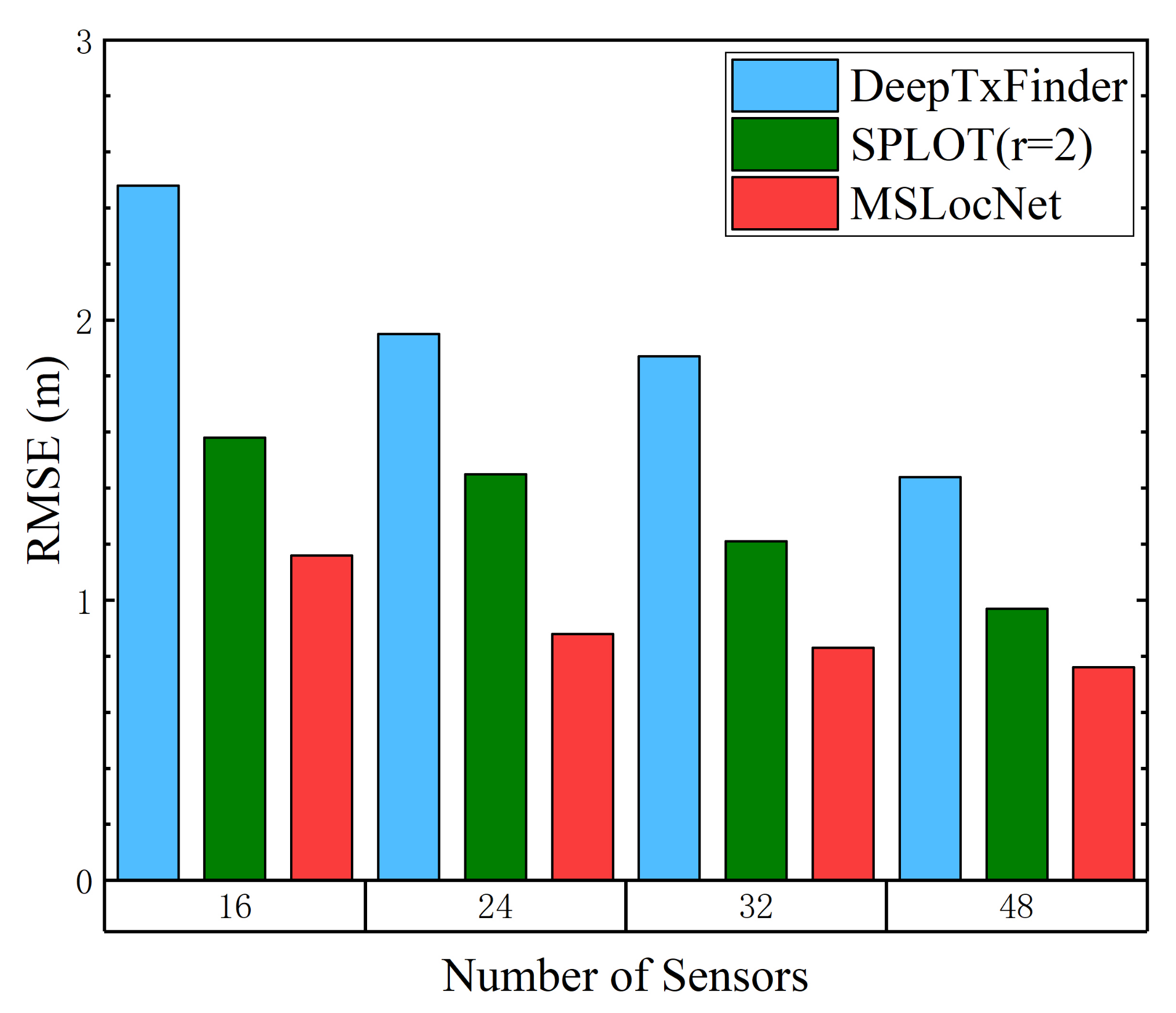
4.1.2. Effects of the Number of Sensors

In this section, the influence of sensor density $\alpha$ on localization performance is evaluated. The RMSE for different $\alpha$ when $\sigma =$ 4 dB are presented in Figure 7. It is observed that the RMSE of all algorithms decreases as the number of sensors increases, and can converge to accepted localization error in the order of a few meters with $0.25$∼$1\%$ sensor density. For a very low sensor density of 0.028%, all algorithms perform badly (in comparison with higher sensor densities), which is reasonable since less information is obtained, leading to greater uncertainty in the estimates. Although at low sensor density ($\alpha <0.0625\%$), there is no significant difference in performance between the proposed method and the other methods. When the sensor density is 0.028%, the RMSE of the SPLOT (r = 6) method is slightly lower than our proposed MSLocNet. However, as the sensor density increases, the localization performance of the proposed method is significantly improved. Except at the lowest sensor density (i.e., 0.028%), the proposed method exhibits the best localization performance compared to other methods, which means the proposed MSLocNet requires fewer sensors at the same RMSE level.

4.2. Real Experiment

To further verify the feasibility of the proposed method, a real experiment is carried out. The real experiment site with a size of 9 m × 9 m is shown in Figure 8. The experimental area is divided into 1 m × 1 m grid cells, and we collected the RSS in different grid cells. A total of 12 groups of data are collected, each with a source placed at a different location. An Agilent signal generator is used as the radiation source to transmit a single tone signal with a transmission frequency of 500 MHz and transmission power of 15 dBm. In our experiment, the radiation signal is collected by HackRF One, a software-defined radio (SDR) platform. The signal is downconverted and then sampled at a frequency of 8MSPS. The RSS is calculated by performing a Fast Fourier Transform (FFT) operation on the I/Q signals collected over a certain duration, where the duration time is set to 2 s. Both the transmitting and receiving antennas are omnidirectional antennas with a gain of 1 dBi.

Figure 9 shows the RMSE under the different number of sensors (by calculating the mean RMSE of 12 groups of data) when compared with the SPLOT method (the radius r of the confined area is set to 2) and the DeepTxFinder method. Similar to Section 4.1.2, the localization performance of all algorithms also increases as the number of sensors increases. Compared with the SPLOT (r = 2) method and DeepTxFinder method, the proposed MSLocNet exhibits better localization performance. In addition, the SPLOT (r = 2) method performs better than the DeepTxFinder method. Due to the large amount of parameters in the fully connected layers of DeepTxFinder, it is prone to overfitting, which makes its generalization performance poor. When the number of the sensor is 16, the RMSE of all algorithms is large than 1 m. However, as the number of sensors increases, the proposed MSLocNet outperforms the other schemes by a large margin. The RMSE of the proposed MSLocNet can reach less than 1 m when the number of sensors is more than 24, which preliminarily verifies the feasibility of the proposed method in the actual environment. Although, the log-normal shadow fading propagation model in Equation (1) can provide an approximation of the decay of electromagnetic energy. However, in a real-time electromagnetic environment, the measurements may not perfectly match the propagation model, which may lead to an increase in RMSE values over those obtained from simulated data. In addition, for practical use, more data from the real environment can be collected to retrain or fine-tune the network for better performance.

5. Conclusions

In this paper, the RSS-based multiple co-channel sources localization problem utilizing deep learning technology is investigated. The proposed method named MSLocNet formulates the MSL problem as a Bernoulli heatmap learning problem, which is to learn a non-linear mapping function from the input sensing data to a heatmap. The Bernoulli heatmap problem is solved by constructing a fully convolutional network. The proposed method can simultaneously localize variable numbers of sources using only one network. Simulation results under different shadow fading strengths illustrate that the proposed MSLocNet is superior to other benchmark schemes. Furthermore, a preliminary experiment in a real environment is performed to verify the feasibility of the proposed method. In the future, more rigorous analyses and comprehensive experiments will be conducted for practical application. Moreover, we plan to extend our approach to different propagation models and develop techniques to reduce training costs and optimize sensor deployment.

References

1. Saeed, N.; Nam, H.; Al-Naffouri, T.Y.; Alouini, M.S. A State-of-the-Art Survey on Multidimensional Scaling-Based Localization Techniques. IEEE Commun. Surv. Tutor. 2019, 21, 3565–3583. [Google Scholar] [CrossRef] [Green Version]
2. Zekavat, R.; Buehrer, R.M. Wireless Positioning Systems: Operation, Application, and Comparison; John Wiley & Sons: Hoboken, NJ, USA, 2019; pp. 3–23. [Google Scholar] [CrossRef]
3. Shen, H.; Ding, Z.; Dasgupta, S.; Zhao, C. Multiple Source Localization in Wireless Sensor Networks Based on Time of Arrival Measurement. IEEE Trans. Signal. Process. 2014, 62, 1938–1949. [Google Scholar] [CrossRef]
4. Zhang, Y.; Wu, Y.I. Multiple Sources Localization by the WSN Using the Direction-of-Arrivals Classified by the Genetic Algorithm. IEEE Access 2019, 7, 173626–173635. [Google Scholar] [CrossRef]
5. Hu, Y.; Abhayapala, T.D.; Samarasinghe, P.N. Multiple Source Direction of Arrival Estimations Using Relative Sound Pressure Based MUSIC. IEEE/ACM Trans. Audio Speech Lang. Process. 2021, 29, 253–264. [Google Scholar] [CrossRef]
6. Ye, X.; Rodríguez-Piñeiro, J.; Liu, Y.; Yin, X.; Pérez Yuste, A. A novel experiment-free site-specific TDOA localization performance-evaluation approach. Sensors 2020, 20, 1035. [Google Scholar] [CrossRef] [PubMed] [Green Version]
7. You, K.; Guo, W.; Peng, T.; Liu, Y.; Zuo, P.; Wang, W. Parametric Sparse Bayesian Dictionary Learning for Multiple Sources Localization with Propagation Parameters Uncertainty. IEEE Trans. Signal. Process. 2020, 68, 4194–4209. [Google Scholar] [CrossRef]
8. Tang, R.; Zhang, Q.; Zhang, W.; Ma, H. Sparse Bayesian multiple sources localization using variational approximation for Laplace priors. Digit. Signal Process. 2022, 126, 103460. [Google Scholar] [CrossRef]
9. Mazuelas, S.; Bahillo, A.; Lorenzo, R.M.; Fernandez, P.; Lago, F.A.; Garcia, E.; Blas, J.; Abril, E.J. Robust Indoor Positioning Provided by Real-Time RSSI Values in Unmodified WLAN Networks. IEEE J. Sel. Top. Signal Process. 2009, 3, 821–831. [Google Scholar] [CrossRef]
10. Patwari, N.; Hero, A.; Perkins, M.; Correal, N.; O’Dea, R. Relative location estimation in wireless sensor networks. IEEE Trans. Signal. Process. 2003, 51, 2137–2148. [Google Scholar] [CrossRef] [Green Version]
11. Coluccia, A.; Ricciato, F. On ML estimation for automatic RSS-based indoor localization. In Proceedings of the IEEE 5th International Symposium on Wireless Pervasive Computing 2010, Mondena, Italy, 5–7 May 2010; pp. 495–502. [Google Scholar] [CrossRef]
12. Tomic, S.; Beko, M.; Dinis, R.; Lipovac, V. RSS-based localization in wireless sensor networks using SOCP relaxation. In Proceedings of the 2013 IEEE 14th Workshop on Signal Processing Advances in Wireless Communications (SPAWC), Darmstadt, Germany, 16–19 June 2013; pp. 749–753. [Google Scholar] [CrossRef]
13. Tomic, S.; Beko, M.; Dinis, R. RSS-Based Localization in Wireless Sensor Networks Using Convex Relaxation: Noncooperative and Cooperative Schemes. IEEE Trans. Veh. Technol. 2015, 64, 2037–2050. [Google Scholar] [CrossRef] [Green Version]
14. Chu, Y.; You, K.; Guo, W. Multiple Sources Localization with Sparse Recovery under Log-normal Shadow Fading. arXiv 2021, arXiv:2105.15097. [Google Scholar]
15. Feng, C.; Valaee, S.; Tan, Z. Multiple target localization using compressive sensing. In Proceedings of the GLOBECOM 2009—2009 IEEE Global Telecommunications Conference, Honolulu, HI, USA, 30 November–4 December 2009; pp. 1–6. [Google Scholar] [CrossRef]
16. Heyde, C.C. On a property of the lognormal distribution. J. R. Stat. Soc. Ser. B Methodol. 1963, 25, 392–393. [Google Scholar] [CrossRef]
17. Fenton, L. The Sum of Log-Normal Probability Distributions in Scatter Transmission Systems. IRE Trans. Commun. Syst. 1960, 8, 57–67. [Google Scholar] [CrossRef]
18. Wang, G.; Chen, H.; Li, Y.; Jin, M. On Received-Signal-Strength Based Localization with Unknown Transmit Power and Path Loss Exponent. IEEE Wirel. Commun. Lett. 2012, 1, 536–539. [Google Scholar] [CrossRef]
19. Khaledi, M.; Khaledi, M.; Sarkar, S.; Kasera, S.; Patwari, N.; Derr, K.; Ramirez, S. Simultaneous power-based localization of transmitters for crowdsourced spectrum monitoring. In Proceedings of the 23rd Annual International Conference on Mobile Computing and Networking, Snowbird, UT, USA, 16–20 October 2017; pp. 235–247. [Google Scholar]
20. Zubow, A.; Bayhan, S.; Gawłowicz, P.; Dressler, F. DeepTxFinder: Multiple transmitter localization by deep learning in crowdsourced spectrum sensing. In Proceedings of the 2020 29th International Conference on Computer Communications and Networks (ICCCN), Honolulu, HI, USA, 3–6 August 2020; pp. 1–8. [Google Scholar] [CrossRef]
21. Papandreou, G.; Zhu, T.; Kanazawa, N.; Toshev, A.; Tompson, J.; Bregler, C.; Murphy, K. Towards accurate multi-person pose estimation in the wild. In Proceedings of the IEEE Conference on Computer Vision and Pattern Recognition, Honolulu, HI, USA, 21–26 July 2017; pp. 4903–4911. [Google Scholar]
22. Chen, Y.; Wang, Z.; Peng, Y.; Zhang, Z.; Yu, G.; Sun, J. Cascaded pyramid network for multi-person pose estimation. In Proceedings of the 2018 IEEE/CVF Conference on Computer Vision and Pattern Recognition, Salt Lake City, UT, USA, 18–22 June 2018; pp. 7103–7112. [Google Scholar] [CrossRef] [Green Version]
23. Zhou, T.; Wang, W.; Liu, S.; Yang, Y.; Van Gool, L. Differentiable multi-granularity human representation learning for instance-aware human semantic parsing. In Proceedings of the IEEE/CVF Conference on Computer Vision and Pattern Recognition, Nashville, TN, USA, 20–25 June 2021; pp. 1622–1631. [Google Scholar]
24. Uko, M.C.; Ukommi, U.S.; Ekpo, S.C.; Kharel, R. Area spectral efficiency of a macro-femto heterogeneous network for cell-edge users under shadowing and fading effects. Appl. Comput. Electromagn. Soc. J. 2016, 31, 1043–1047. [Google Scholar]
25. Cui, M.; Cha, H.; Tian, B. A propagation model for rough sea surface conditions using the parabolic equation with the shadowing effect. Appl. Comput. Electromagn. Soc. J. 2018, 33, 683–689. [Google Scholar]
26. He, K.; Zhang, X.; Ren, S.; Sun, J. Deep residual learning for image recognition. In Proceedings of the IEEE Conference on Computer Vision and Pattern Recognition, Las Vegas, NV, USA, 26 June–1 July 2016; pp. 770–778. [Google Scholar]
27. Ioffe, S.; Szegedy, C. Batch normalization: Accelerating deep network training by reducing internal covariate shift. In Proceedings of the International Conference on Machine Learning (ICML), Lille, France, 6–11 July 2015; pp. 448–456. [Google Scholar]
28. Hinton, G.; Srivastava, N.; Swersky, K. Neural Networks for Machine Learning Lecture 6a Overview of Mini-Batch Gradient Descent. 2012. Available online: https://www.cs.toronto.edu/~tijmen/csc321/slides/lecture_slides_lec6.pdf (accessed on 5 May 2022).
Figure 1. The scenario of multiple sources localization.
Electronics 11 01551 g001
Figure 2. Overview architecture for MSLocNet.
Electronics 11 01551 g002
Figure 3. (a) Heatmap with ideal delta functions; (b) heatmap with a region of radius R without quantization error; (c) heatmap with a region of radius R with quantization error.
Electronics 11 01551 g003
Figure 4. (a) MSLocNet structure; (b) convolution module; (c) ResBlock structure; (d) Upsampling layer structure (we observe that a five-layer model produces good results and tried adding more layers, but it did not lead to significant improvement).
Electronics 11 01551 g004
Figure 5. The RMSE for different σ .
Electronics 11 01551 g005
Figure 6. The examples of the predicted heatmap: (a) the number of radiation sources is 1; (b) the number of radiation sources is 2; (c) the number of radiation sources is 3.
Electronics 11 01551 g006
Figure 7. The RMSE for different α .
Electronics 11 01551 g007
Figure 8. The site of real experiment.
Electronics 11 01551 g008
Figure 9. The RMSE (m) for real data.
Electronics 11 01551 g009
Publisher’s Note: MDPI stays neutral with regard to jurisdictional claims in published maps and institutional affiliations.