A Novel Two-Stage Deep Learning Structure for Network Flow Anomaly Detection

Abstract

Unknown cyber-attacks have appeared constantly. Several anomaly detection techniques based on semi-supervised learning have been proposed to detect these unknown cyber-attacks. Among them, the Denoising Auto-Encoder (DAE) scheme performs better than others in accuracy but is not good enough in precision. This paper proposes a novel two-stage deep learning structure for network flow anomaly detection by combining the models of Gate Recurrent Unit (GRU) and DAE. By using supervised anomaly detection with a selection mechanism to assist semi-supervised anomaly detection, the precision and accuracy of the anomaly detection system are improved. In the proposed structure, we first use the GRU model to analyze the network flow and then take the outcome from the Softmax function as a confidence score. When the score is more than or equal to the predefined confidence threshold, the GRU model outputs the flow as a positive result, no matter the flow is classified as normal or abnormal. When the score is less than the confidence threshold, GRU model outputs the flow as a negative result and passes the flow to DAE model for flow classification. DAE then determines a reconstruction error threshold by learning the pattern of normal flows. Accordingly, the flow is normal or abnormal depending on whether it is under or over the reconstruction error threshold. A comparative experiment is performed using NSL-KDD dataset as benchmark. The results revealed that the precision using the proposed scheme is 0.83% better than DAE. The accuracy using the proposed approach is 90.21%, which is better than Random Forest, Naïve Bayes, One-Dimensional Convolutional Neural Network, two-stage Auto-Encoder, etc. In addition, the proposed approach is also applied to the environment of software defined network (SDN). By adopting our approach in SDN environment, the precision and F-measure are significantly improved.

1. Introduction

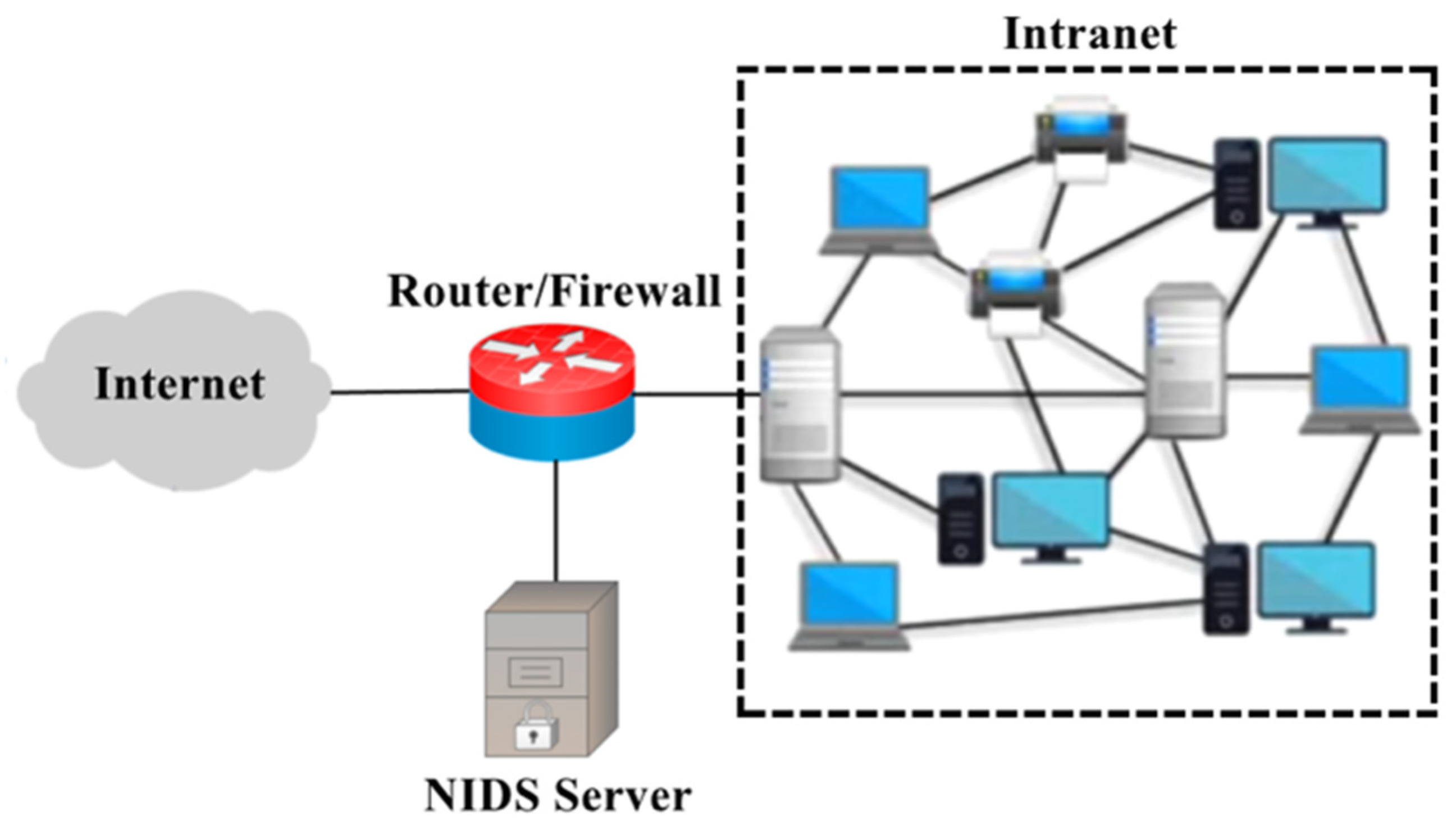
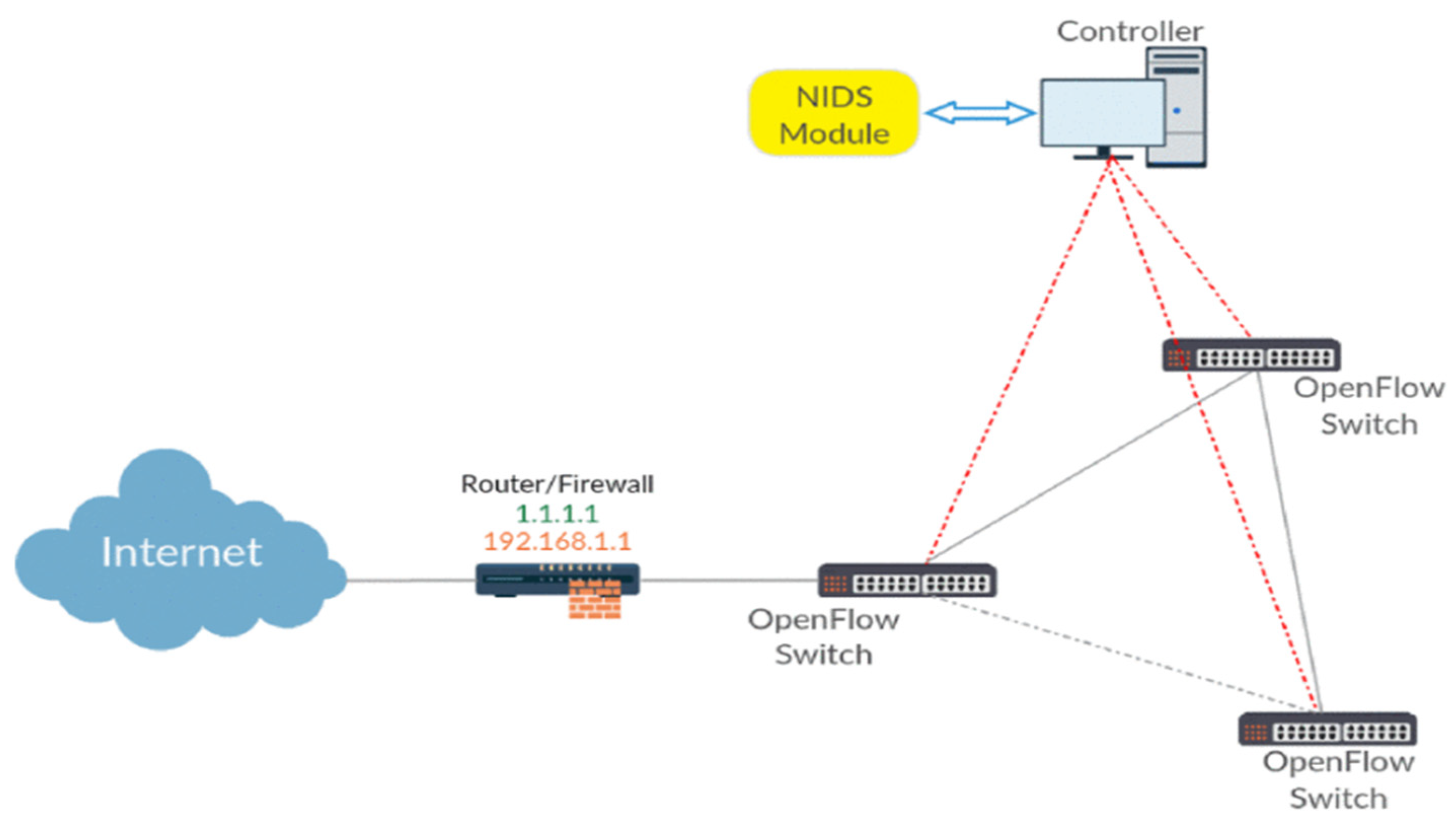
In recent years, due to the massive increase in the number of unknown attacks, the development of a network intrusion detection system (NIDS) that effectively resists unknown attacks is an important topic for the network administrator [1]. As shown in Figure 1, the NIDS server is deployed at the entrance of the connection between the Intranet and the Internet. It monitors the network packets flowing into the Intranet, analyzes statistical data collected from network flows, and uses detection mechanisms to determine if the flows are normal or abnormal. This method can help network managers find abnormal network conditions and then quickly take defensive measures.

The detection scheme of the NIDS can be divided into signature-based intrusion detection and anomaly-based intrusion detection. The former is currently the main detection scheme of commercial NIDS, such as Snort and Suricata. This scheme analyzes the patterns or behaviors of past attack flow samples by experts, writes the analysis results into the flow judging rules, and compares the incoming flow with features to determine whether it conforms to the attack behavior or not. With this scheme, the rate of misjudgment is low, but it is difficult to detect unknown network attacks. The latter uses machine learning or deep learning methods to train a classifier model through a mixture of abnormal and normal flows. This method is easier to detect unknown attacks, but the accuracy is low. On a real network, it is very difficult and time-consuming to label the flow types one by one. Under normal circumstances, most of the available flow samples belong to normal flow. To train the classifier from a small number of abnormal flow samples may cause poor classification results and a high misjudging rate. Unknown attacks easily evade the use of signature-based intrusion detection systems, causing harm to users. Based on the above situations, most researchers use anomaly-based intrusion detection as the detection scheme of NIDS.

V. Chandola et al. [2] pointed out that according to different learning methods, anomaly detection schemes are divided into three categories, supervised anomaly detection (SAD), semi-supervised anomaly detection (SSAD), and unsupervised anomaly detection (UAD). First, the SAD scheme uses supervised learning to train the detection model with labeled samples (marked with normal or abnormal flow). Typical examples of SAD mechanisms include common convolutional neural networks (CNN) [3,4], recurrent neural networks (RNN) [5], LSTM [6], decision trees, random forests, Bayesian classifiers, etc. The learning effect of SAD is very good, but due to the limited number of labeled samples, usually only limited abnormal states can be learned. Next, the SSAD scheme is only trained with samples of normal behavior. By learning the behavior patterns of samples with normal flow, it is highly sensitive to unknown abnormal flow. Typical examples of SSAD mechanisms include Auto-Encoder (AE) [7,8], One Class-SVM [9], and Denoising Auto-Encoder (DAE) [10]. Finally, the UAD mechanism directly trains using unlabeled flow samples. This method must assume that the number of normal flow samples in all flow samples is much larger than abnormal flow samples, and the behavior patterns of abnormal flow samples cannot be too similar to normal flow samples. Without the above premise, the model trained by this method will result in a higher misjudging rate.

As mentioned above, current research tends to use SSAD schemes as the detection model of NIDS. For those SSAD schemes, we perform an experiment and find that the overall accuracy of the DAE model is better than other approaches. We also find that although the overall accuracy of the DAE model is very high, the probability of judging normal flow as abnormal is also higher than that of the supervised model; that is, the precision of the DAE model is lower. To improve the overall accuracy and precision, this paper proposes a two-stage anomaly detection and judging structure by combining SAD and SSAD schemes. To pick our first-stage detection model, we first select two SAD schemes, Gate Recurrent Unit (GRU) [11] and One-Dimensional Convolutional Neural Network (1DCNN) [12], together with the DAE model to form a two-stage model and compare them in terms of accuracy. The experimental results show the overall accuracy of the GRU model is better. Therefore, we pick up the GRU model as our first-stage detection model.

In the proposed structure, we first use the GRU model to analyze the network flow and then take the outcome from the Softmax function as a confidence score. When the score is more than or equal to the predefined confidence threshold, the GRU model outputs the flow as a positive result, no matter whether the flow is classified as normal or abnormal. When the score is less than the confidence threshold, the GRU model outputs the flow as a negative result and passes the flow to the DAE model for flow classification. DAE then determines a reconstruction error threshold by learning the pattern of normal flows. Accordingly, the flow is normal or abnormal depending on whether it is under or over the reconstruction error threshold. We train and test the proposed system by using the benchmark dataset NSL-KDD [13]. In NSL-KDD dataset, the flow is divided into normal flow and abnormal flow, and 41 features are used for training. On the other hand, due to the rapid development of Software Defined Network (SDN) in recent years, we also apply the proposed structure in the SDN network and compare it with other IDS systems applied to SDN [14] by using the NSL-KDD dataset as the benchmark. Note that because of the characteristics of SDN environment, only nine features of the NSL-KDD dataset are selected to form the benchmark dataset.

The rest of this paper is organized as follows. Dataset used in this paper and related studies are given in Section 2. In Section 3, the proposed scheme is presented. Simulation and performance evaluation are given in Section 4. Finally, we give a conclusion.

2. Datasets and Related Studies

2.1. Datasets for NIDS

One of the more famous datasets in the field of NIDS is KDD 99 [15], which was used when the KDD Cup was held in 1999. In 2009, the NSL-KDD dataset was published by M. Tavallaee et al. [13], which improved the shortcoming of the KDD 99 dataset, which contains too many duplicate samples and removes the samples that are too easy to identify. It is currently one of the main datasets for evaluating the performance of NIDS. Its feature is that the test dataset contains attack flow that has not appeared in the training dataset. According to A. Aldweesh et al. [16], as shown in Figure 2, most current research uses KDD99 and NSL-KDD as a dataset for evaluating performance. Among them, NSL-KDD accounted for the majority. Therefore, this paper uses the NSL-KDD as the benchmark dataset.

In the NSL-KDD dataset, each sample is a flow sample collected through flow analysis. Like the KDD 99 dataset, it contains 41 features and 1 flow type name. In addition to normal flow, there are 39 types of attack flow. These attack types are divided into four classes: Denial of Service (DoS); Remote to Local (R2L); User to Root (U2R); and Probe. In the DoS class, the attacker forces the target machine to suspend the service in some way, such as occupying network bandwidth or consuming memory resources; thus that legitimate users cannot use the service and access resources. In the R2L class, the attacker steals the user’s password and personal information remotely against the target user’s own system vulnerabilities, or the password strength is too low. In U2R class, an attacker who has obtained a general user account has unauthorized access to root privileges. In the Probe class, the attacker monitors the network packets passing by the target machine to find information and vulnerabilities that are beneficial to the attack. The attack types of the NSL-KDD dataset are shown in

Table 1. The attack types of the NSL-KDD dataset.

Types	Attack Name
DoS	back, land, neptune, pod, sumrf, teardrop, apache2, mailbomb, processtable, udpstorm
R2L	ftp_write, guess_passwd, imap, multihop, phf, spy, warezclient, warezmaster, named, sendmail, snmpgetattack, snmpguess, worm, xlock, xsnoop
U2R	buffer_overflow, loadmodule, perl, rootkit, httptunnel, ps, sqlattack, xterm
Probe	ipsweep, nmap, portsweep, satan. mscan, saint

.

The features of the NSL-KDD dataset can be divided into three classes: Basic Features; Content Features; and Flow Features. The features and flow name of NSL-KDD dataset are sorted in order. Numbers 1 to 9 are the basic features, which are indicating the basic information of the packet header when connecting. For example, protocol_type is the network protocol used by the connection. Numbers 10 to 22 are content features, which are commonly used features in the field of NIDS. For example, num_failed_logins is the number of system connection login failures. The flow features are divided into time-based statistical features (No. 23 to No. 31) and host connection statistics-based features (No. 32 to No. 41). The last one, number 42, is the name of the flow type.

2.2. Related Studies

We mentioned in the introduction that an anomaly-based intrusion detection system can be divided into SAD, SSAD, and UAD. Due to the numerous research on NIDS, it is very difficult to find datasets and evaluation indicators that can compare all methods. Therefore, this paper collects multiple articles that use the NSL-KDD dataset as a benchmark with the accuracy results. These relevant pieces of research are included in the comparison in terms of accuracy.

Table 2. A variety of methods used the accuracy of the NSL-KDD test dataset.

Method	Type of Learning	Accuracy (%)
Decision Tree [13]	Supervised	81.07
Naïve Bayes [13]	Supervised	75.56
Random Forest [13]	Supervised	80.67
RNN [5]	Supervised	83.28
1DCNN [17]	Supervised	84.29
SAE + SMR [18]	Hybrid	88.39
SAE + SVM [19]	Hybrid	84.96
AE [7]	Semi-Supervised	88.28
DAE [7]	Semi-Supervised	88.65
SAE-AE [21]	Semi-Supervised	90.17

summarizes the accuracy results of different methods using the NSL-KDD dataset as a benchmark. The accuracy of traditional machine learning, such as decision tree (J48) [10], Naive Bayes classifier [13], and Random Forest [13] are 81.07%, 75.56%, and 80.67%, respectively. The accuracy of supervised deep learning 1DCNN [17] and RNN [5] are 83.28% and 84.29%, respectively. Q. Niyaz et al. [18] and M. Al-Qatf et al. [19] used Sparse Auto-Encoder (SAE) [20] to learn deep features and then trained with a supervised learning method; the results were 88.39% and 84.96 %, both using autoencoders for feature extraction. R.C.Aygun et al. [7] used Denoising Auto-Encoder (DAE) with an accuracy of 88.65%, which was the single semi-supervised anomaly detection model with the best accuracy found in the NSL-KDD test set for this study. M. Gharib et al. [21] proposed the two-stage auto-encoder architecture as the current best overall accuracy. This method uses the auto-encoder to learn the normal flow and evaluates the abnormal flow by calculating reconstruction errors. Some methods use more than two learning methods, such as M.Al-Qatf et al. [19] using unsupervised SAE with supervised Support Vector Machine (SVM). This paper also uses supervised GAU models with semi-supervised DAE. In order to facilitate the interpretation, the learning type was marked as a hybrid.

Moreover, D. Santhadevi and B. Janet [22] proposed an EIDIMA framework, which used machine learning techniques, an input vector databank, a decision-making module, and a subsample module for traffic categorization at edge devices. EIDIMA’s classification performance was assessed using the F1-Score, accuracy, recall, and precision. Devarakonda et al. [23] outlined and compared four AI methods to train two benchmark datasets—the KDD′99 and the NSL-KDD. Deswal et al. [24] provided a hybrid intrusion detection system that combined distinguished machine learning models such as convolution neural network (CNN), residual network, and multilayer perceptron. Their results revealed that deep CNN with higher accuracy of 0.93 on the NSL-KDD dataset. Sun et al. [25] proposed a deep convolutional neural network model based on Resnet (Residual Network) to solve the problem of insufficient detection ability of massive network intrusion data and a few attack samples for intrusion detection. They also used the NSL-KDD dataset as a benchmark dataset.

3. Two-Stage Deep Learning Structure for Network Flow Anomaly Detection

In order to improve the accuracy and precision of the DAE model, this paper uses a SAD model to assist the DAE model. Among several SAD models, the accuracy of GRU and 1DCNN models performed better than other approaches. For both models, we performed an experiment on them and found that the GRU model could improve the accuracy and precision simultaneously; thus, we chose the GRU model and DAE to form a two-stage deep learning anomaly detection structure. In the proposed structure, we first used the GRU model to analyze the network flow and then took the outcome from the Softmax function as a confidence score. When the score is more than or equal to the predefined confidence threshold, the GRU model outputs the flow as a positive result, no matter whether the flow is classified as normal or abnormal. When the score is less than the confidence threshold, the GRU model outputs the flow as a negative result and passes the flow to the DAE model for flow classification. DAE then determines a reconstruction error threshold by learning the pattern of normal flows. Accordingly, the flow was normal or abnormal depending on whether it was under or over the reconstruction error threshold. The two models add a hidden layer of two neurons when designing the neural network architecture to facilitate subsequent data visualization actions and facilitate the interpretation of researchers.

3.1. Data Preprocessing

Data preprocessing is a very important stage in machine learning. There are different data preprocessing schemes for the features of different data types. Usually, continuous features use feature scaling to scale different features into the same comparison interval, and discrete features use coding methods to classify different types of data. This paper applies Min-Max normalization for continuous features. It is assumed that a sample contains multiple continuous features, and different features have different numerical ranges. By scaling each feature to a fixed size, the training will not be biased for some features. The equation of Min-Max normalization is shown in Equation (1), where x is the actual value of a sample in the feature to be calculated; min(x) and max(x) are the minimum and maximum values of the features in the overall sample, respectively. The normalized value x′ is calculated by the Equation (1), which can compress the features of different sizes in the range of 0 to 1. With the Min-Max normalization, the data consistency is improved.

$${𝓍}^{\prime }=\frac{x-\min \left(𝓍\right)}{\max \left(𝓍\right)-\min \left(𝓍\right)}$$

(1)

Commonly used encoding methods include label encoding and one hot encoding. The label encoding will sequentially encode the newly emerging categories as integers from small to large. This method is fast and does not increase the number of features, but the labeled types are all in the same feature and presented as integers. The one-hot encoding separates each category in the feature into individual features. The disadvantage of one-hot encoding is that the number of features increases according to the number of types in the original feature, but it is easier to learn the content of the feature compared to label encoding. If the added feature is still within the normal range, it is still the most current machine learning mainstream method used in the research. Therefore, in this paper, one-hot encoding scheme is used for discrete features.

3.2. Operational Process of Training and Judging Mode

Two modes, training mode and judging mode, are included in the proposed structure. Each mode consists of two modules, the GRU module, and the DAE module. The detailed operational processes are presented in the following subsections.

3.2.1. Operational Process of Training Mode

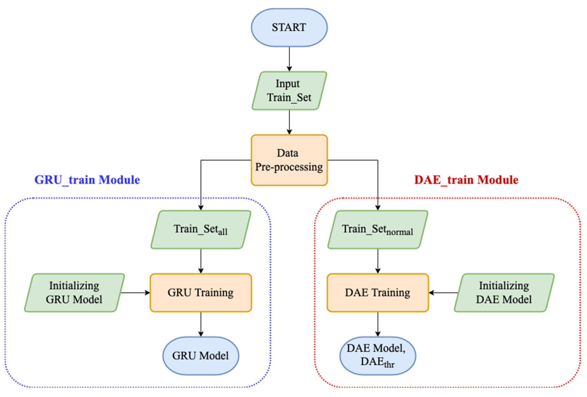
Figure 3 presents the operational process of the training mode. $Train\_Set$ denote the complete training set flow sample. The data will be preprocessed and converted the features into a format suitable for deep learning. We classified those data into two sets of training samples, $Train\_Se{t}_{all}$ and $Train\_Se{t}_{normal},$ where the set of $Train\_Se{t}_{all}$ included all labeled normal and abnormal flow samples and the set of $Train\_Se{t}_{normal}$ included labeled normal flow samples. The set of $Train\_Se{t}_{all}$ will be inputted to the GRU_train module as the initialized training sample of GRU model. After the training being completed, the GRU model has learned normal and abnormal flow samples. The set of $Train\_Se{t}_{normal}$ will be inputted to the DAE_train module as the initialized training sample of DAE model. After the training is completed, the DAE model has learned normal flow samples. The reconstruction error of the last training epoch will be taken as the DAE reconstruction error threshold Value ($DA{E}_{thr}$).

3.2.2. Operational Process of Judging Mode

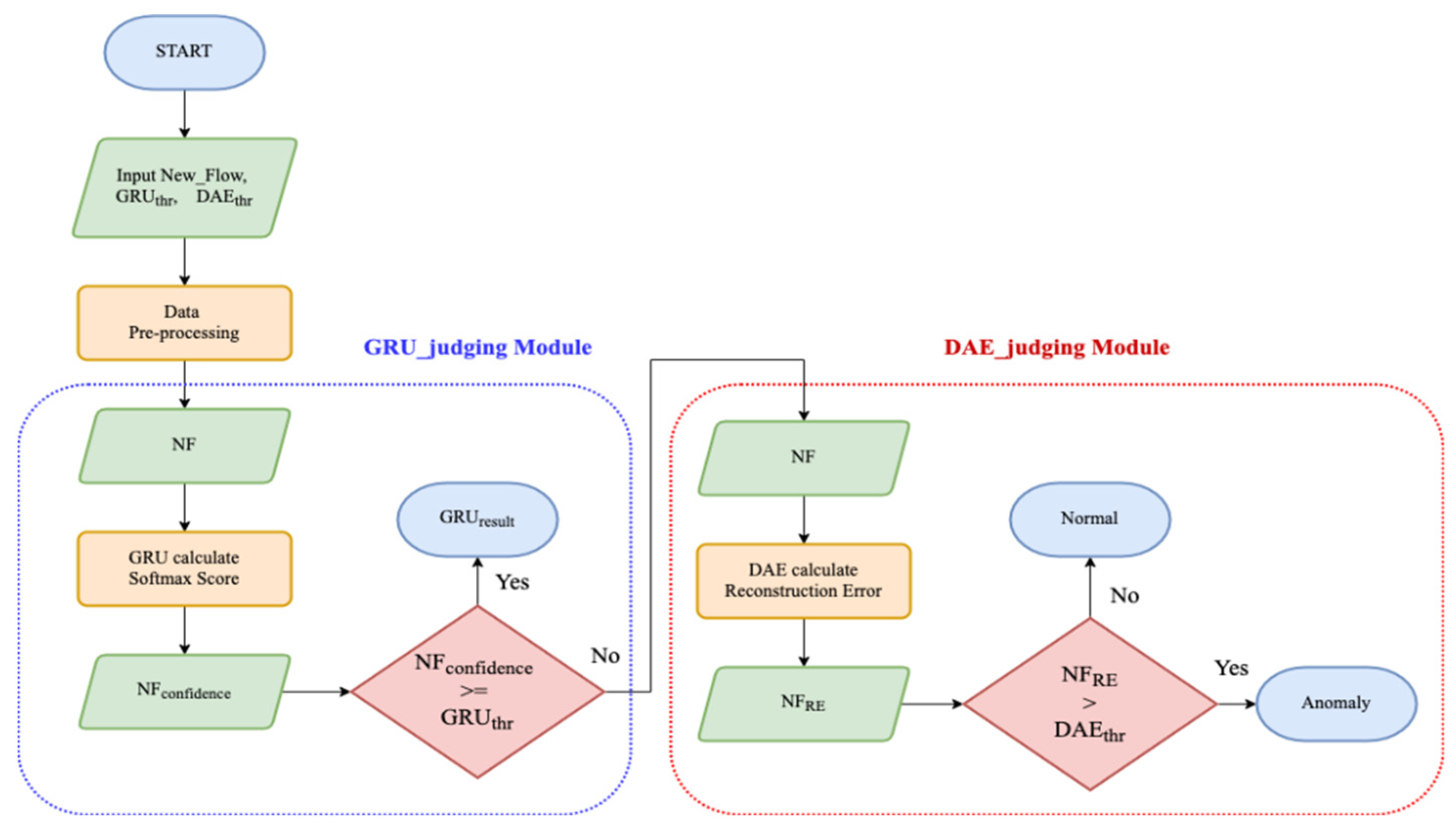
The operational process of the judging mode is shown in Figure 4. At the beginning of the process, we first have to set the GRU confidence threshold ($GR{U}_{thr}$) and DAE reconstruction error threshold ($DA{E}_{thr}$). $GR{U}_{thr}$ can be set by experience, and $DA{E}_{thr}$ is automatically learned by the DAE_train module during training mode. When the judging mode operates, the new flow (New_Flow) will be allowed to enter, and after data is preprocessed, a flow sample (NF) suitable for deep learning is generated. In the first stage, GRU_judging module, the GRU model will calculate the Softmax score for the NF as the confidence score $N{F}_{confidence}$, and then compare it with the previously set $GR{U}_{thr}$. If the value of $N{F}_{confidence}$ is greater than or equal to the value of $GR{U}_{thr}$, it means that the GRU module has sufficient confidence this time. The GRU_judging module will output the result, $GR{U}_{result}$, and then end the judgment. If the value of $N{F}_{confidence}$ is lower than value of $GR{U}_{thr}$, the NF will be passed to the second stage, DAE_judging module, for making a judgment. The DAE_judging module calculates the reconstruction error $N{F}_{RE}$ for the NF using the DAE model and compares it with $DA{E}_{thr}$. If the value of $N{F}_{RE}$ is higher than $DA{E}_{thr}$, the NF is judged as abnormal flow; otherwise the NF is judged as normal flow.

3.3. Threshold Value Setup and Input Method of GRU

In the GRU model, we used the Softmax score as the confidence score. Softmax is often used in the final output of the classifier model. The Softmax score can be obtained from Equation (2), where exp is the exponential function with Euler numbers e as the base, ${\mathcal{X}}_i$ is the output of the $i$th category, and ${\mathcal{X}}_i$ is divided by all j-types after exponential function calculation. The sum of the exponential function is to calculate the probability value of the $i$th category, and the total probability value of all types j is equal to 1.

$$\mathrm{Softmax}\left({\mathcal{X}}_i\right)=\frac{\exp \left({\mathcal{X}}_i\right)}{{{\displaystyle \sum }}_{i=1}^j\exp \left({\mathcal{X}}_i\right)}$$

(2)

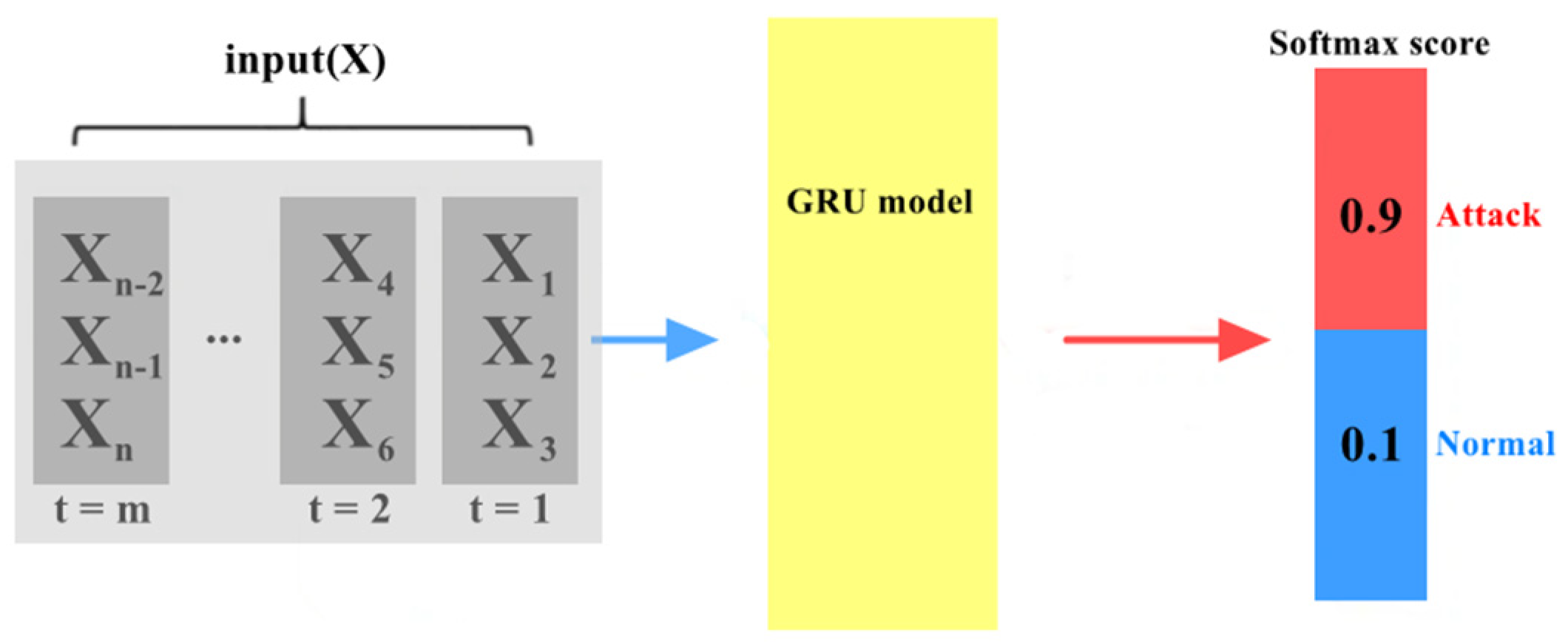
Figure 5 is an example of the GRU model outputting the Softmax score. Because the goal is to separate abnormal flow and normal flow, the GRU model will output a set of two-dimensional vectors, as shown in Figure 5. In Figure 5, the values of 0.9 and 0.1 represent that the GRU model believes that the flow is attack flow with a probability of 0.9 and is normal flow with the probability of 0.1. The larger the probability value, the more confident the model is in the judgment. Therefore, when the confidence threshold is not set, the GRU model will directly output the judging result as abnormal flow. In this paper, once a Softmax score is generated, it has to be compared with the confidence threshold. When the confidence score is greater than or equal to the confidence threshold, the GRU model outputs the result; otherwise, it will be handed over to the next stage of the DAE model for judgment.

Due to the Softmax score outputted by the model will have different output results according to different training cycles, model parameters, and other variables, it is difficult to directly set a fixed confidence threshold. In this paper, the confidence threshold setting is adjusted artificially. We actually test the confidence threshold ranging between 0.99900 and 0.99999 on the NSL-KDD data set. It was found that the confidence threshold of the GRU module in this study was between 0.99984 and 0.99996, which has a good performance on the overall structure. Therefore, we set the confidence threshold as 0.99990.

3.4. Threshold Value Setup of DAE

This paper uses the DAE model as the second-stage detection model. DAE creates the effect of missing values by adding noise to the input data. Let the DAE model learn to restore the original data without missing values from the input data with missing values; thus that the trained model is less likely to overfit. This allows the DAE model to learn the really important features from the data, thereby improving generalization capabilities.

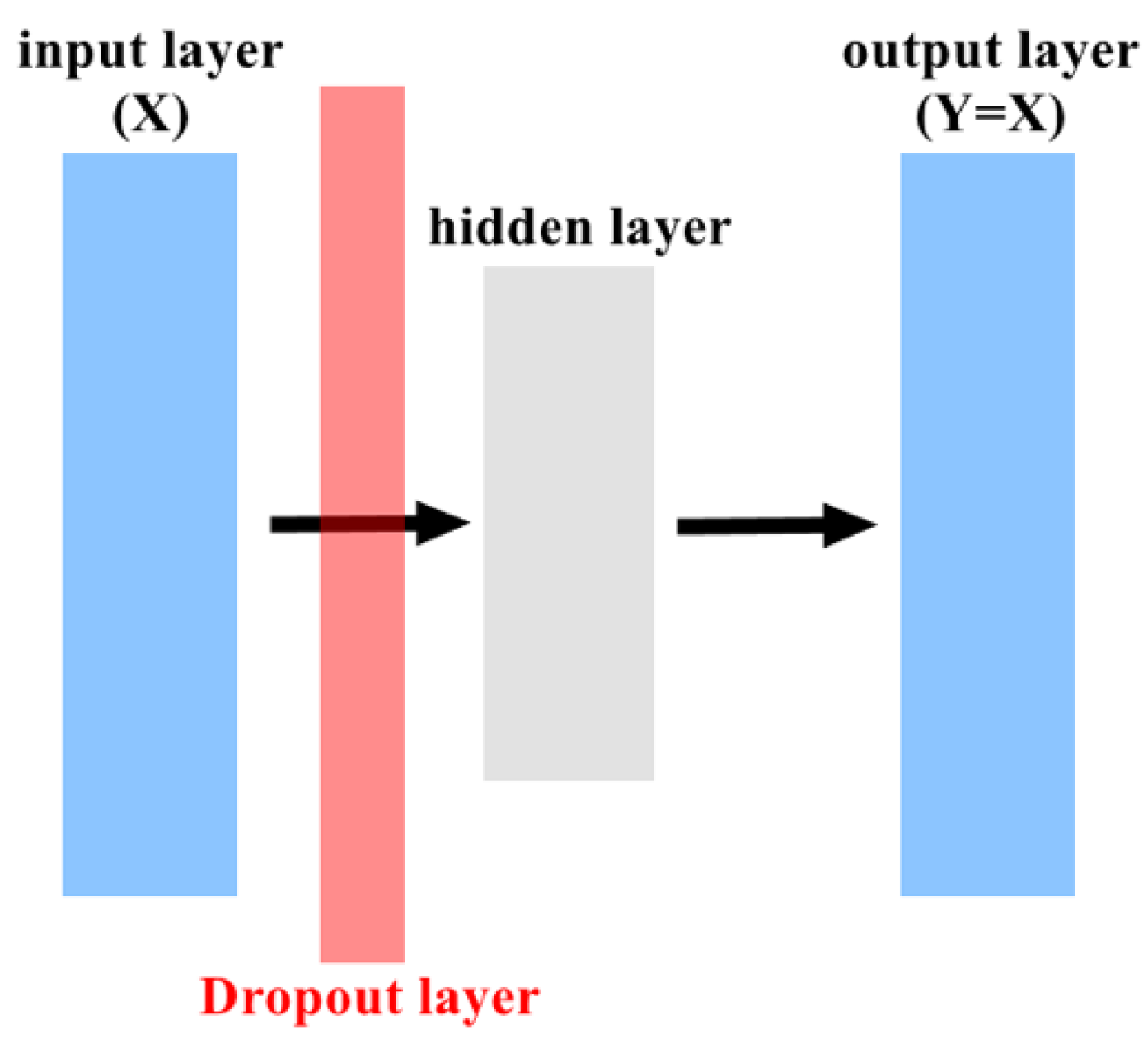
In this paper, we use only one hidden layer in the DAE model, which can also be called the bottleneck layer of the autoencoder. In addition, as shown in Figure 6, we add Dropout [26] between the input layer and the hidden layer. Through Dropout, different input features can be randomly discarded in each batch of training instead of adding noise to the input. The advantage is that it can achieve the effect of training DAE without changing the original data.

The DAE model uses the Mean-Square Error (MSE) loss function to calculate the reconstruction error, as shown in Equation (3). After training, DAE has learned the normal flow behavior pattern and reconstruction error. We use the MSE of the last training period as the reconstruction error threshold. If the calculated MSE of the new flow is higher than the threshold, this new flow will be judged as abnormal.

$$\mathrm{MSE}=\frac{1}{n}{\displaystyle \sum }_{i=1}^n{\left(y_i-{\widehat{y}}_i\right)}^2$$

(3)

3.5. Data Visualization for Softmax Score Selection

Because the network flow data are usually a combination of numerical values and discrete features, observers cannot intuitively understand the results of the model. Therefore, to help observers select and adjust the model, this paper uses the data visualization method to present the neural network model in two-dimensional or even three-dimensional graphics. To conduct that, the bottleneck layer in DAE is set to two neurons. During the prediction, the values of the two neurons in the bottleneck layer of each sample are recorded, and the reconstruction error forms a set of three-dimensional vectors, which are projected on the 3D graphics.

In addition, we also see the last hidden layer of two neurons in the GRU model. The two-dimensional output values of the Softmax score are the probabilities $P_{normal}$ and $P_{anomaly},$ where $P_{normal}$ represents that the probability of the GRU model considers the flow is normal and $P_{anomaly}$ represents that the probability of GRU model considers the flow is abnormal. We convert the two-dimensional output values of the Softmax score into a one-dimensional output value $P_{1d}$. When the value of $P_{normal}$ is greater than the value of $P_{anomaly}$, the value of $P_{1d}$ is equal to the value of $P_{normal};$ otherwise, the value of $P_{1d}$ is equal to the value of $-P_{anomaly}$. Through the process of data visualization, the original two-dimensional outputs are converted into one-dimensional outputs, and finally form a three-dimensional vector with the hidden layer of two neurons and project it on the 3D graphics. The process of data visualization for Softmax score selection is shown is Algorithm 1.

Algorithm 1 Softmax score selection
Inputs:$P_{normal}$, $P_{anomaly}$ Output: $P_{1d}$
1:	if $P_{normal}$ > $P_{anomaly}$ then
2:	$P_{1d}$ = $P_{normal}$
3:	else $P_{1d}$ = $-P_{anomaly}$
4:	return $P_{1d}$

4. Simulation and Performance Evaluation

To verify the feasibility of the proposed scheme, several experiments are carried out on the Google Colab online platform. The Colab development environment and kits are shown in

Table 3. The Colab development environment and kits.

The Colab Development Environment and Kits
OS	Ubuntu 18.04.3 LTS
CPU	Intel Xeon 2.3GHz
GPU	Tesla K80
RAM	13GB
Language	Python3.6
Kits	Tensorflow 2.2.0, Scikit-learn, NumPy, pandas

. We first performed 10 times of training experiments on each of the DAE model and the GRU model using the NSL-KDD dataset and calculated the average accuracy. For those 10 DAE models, we selected the DAE model, in which the accuracy was closed to the average accuracy, to be an exemplary model for presenting data visualization, confusion matrix, and the threshold value. One of the GRU models was selected using a similar way. Finally, we made a comparison between the proposed structure and other approaches in terms of accuracy and precision.

The data distribution of NSL-KDD dataset is shown in

Table 4. Distribution of NSL-KDD dataset.

Types	Number of Samples
	Training Dataset	Test Dataset
Normal	67,343 (53.5%)	9711 (43.1%)
Anomaly	58,630 (46.5%)	12,833 (56.9%)
Total	125,973	22,544

. All four attack types of NSL-KDD dataset were classified as anomalies. The NSL-KDD dataset consists of training set and test set. The total number of samples in the training set was 125,973, in which the number of normal flow samples was 67,343, and the number of abnormal flow samples was 58,630. The total number of samples in the test set was 22,544, in which the number of normal flow samples was 9711, and the number of abnormal flow samples was 12,833. Only normal flow sample in the dataset was used for DAE training and the entire training set was used for GRU training. The discrete data in the NSL-KDD dataset was encoded by one-hot encoding method. After encoding, the total number of features increased from 41 to 126 features.

4.1. Experimental Parameters Setting of DAE Model and GRU Model

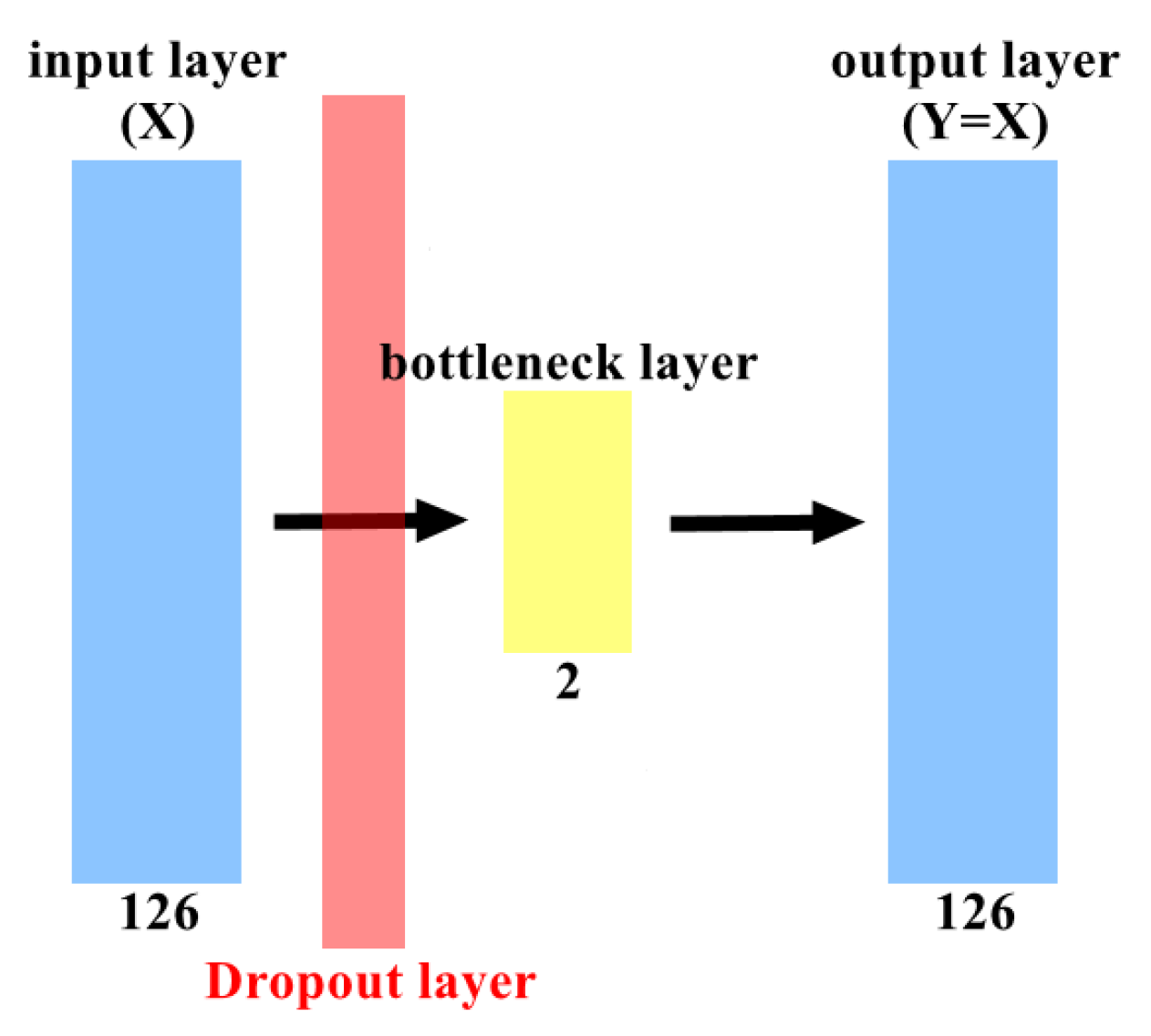
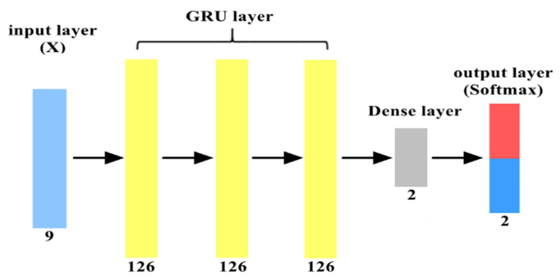
Both DAE and GRU models are shown in Figure 7 and Figure 8, respectively. Note that in both figures, the numbers at the bottom of the layer are the number of neurons used in this layer. In Figure 7, the DAE′s dropout rate is 0.5, which means that half of the features of each batch of input data will be randomly discarded during training. In addition, L2 regularization was added to the bottleneck layer to avoid overfitting. In Figure 8, 126 features were cut into 14-time steps and input in batches, and 9 features were inputted into each time step. This is because, under the input shape of GRU set to (14, 9), the performance of the GRU model was better. The parameters used are shown in

Table 5. The parameters of both models.

	DAE	GRU
Batch Size	256	256
Epochs	100	30
Hidden layer Activation	Sigmoid	Tanh/ReLU
Output layer Activation	Sigmoid	Softmax
Weight Initialization	Glorot uniform	Orthogonal/He normal
Optimizer	Adam	Adam
Loss Function	MSE	Categorical cross-entropy

. In order to improve the fairness of this research, except for the training period, which is a better value selected after testing, the other parameters were commonly used in the two models. Two models were trained 10 times using the NSL-KDD dataset and numbered 1 to 10. In order to facilitate the presentation of experimental results, we calculated the average accuracy of each model and picked the model in which the accuracy was closest to the average accuracy.

4.2. Experimental Results

The experimental results of deep learning usually have a certain degree of randomness, and most studies use accuracy, recall, precision, and F-measure to compare performance. However, few studies show that the final experimental result is obtained after how many experiments or the overall average. In this paper, the final results are obtained based on the average results of 10 experiments.

4.2.1. GRU and DAE Models Training Results

We first performed 10 times of training experiments on each of the GRU model and the DAE model using the NSL-KDD dataset as a benchmark and calculated the average accuracy, the average recall, the average precision, and the average F-measure. The results are shown in

Table 6. Experimental results of the GRU model using the NSL-KDD test dataset as a benchmark.

Model	Accuracy (%)	Precision (%)	Recall (%)	F-Measure (%)
GRU_1	78.49	96.02	64.9	77.45
GRU_2	80.81	95.92	69.24	80.42
GRU_3	78.85	94.05	67.09	78.32
GRU_4	78.38	92.33	67.64	78.08
GRU_5	79.24	92.04	69.55	79.23
GRU_6	77.99	92.28	66.94	77.59
GRU_7	81.12	96.85	69.08	80.64
GRU_8	76.80	92.30	64.63	76.03
GRU_9	78.87	92.32	68.59	78.71
GRU_10	77.57	91.84	66.51	77.15
Average	78.81	93.60	67.42	78.36

and

Table 7. Experimental results of the DAE using the NSL-KDD test dataset as a benchmark.

Model	Accuracy (%)	Precision (%)	Recall (%)	F-Measure (%)
DAE_1	89.70	86.71	96.74	91.45
DAE_2	89.72	86.71	96.77	91.46
DAE_3	88.67	85.46	96.52	90.65
DAE_4	90.02	86.48	97.74	91.77
DAE_5	89.73	86.70	96.81	91.48
DAE_6	89.74	86.69	96.85	91.49
DAE_7	89.91	86.75	97.10	91.64
DAE_8	89.71	86.71	96.75	91.46
DAE_9	89.74	86.72	96.81	91.49
DAE_10	89.72	86.72	96.76	91.47
Average	89.67	86.56	96.89	91.43

, respectively. From both tables, one can see that the accuracy of GRU_3 model and DAE_1 model was closest to the average accuracy. Therefore, both models were selected as exemplary models for presenting data visualization, confusion matrix, and the threshold value.

4.2.2. Data Visualization Results

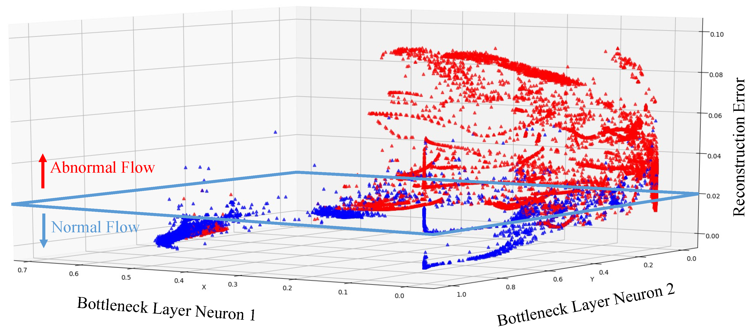
Both the GRU_3 model and the DAE_1 model are visualized with 22544 samples using the complete NSL-KDD test dataset. Figure 9 is the visualization result of the DAE_1 model’s reconstruction error. The red sample is the actual abnormal flow, and the blue sample is the actual normal flow. The x and y axes are the output of two neurons in the bottleneck layer in the DAE, and the z-axis is the reconstruction error of each sample. The DAE_1 model was trained, and then the reconstruction error threshold value was obtained, as shown in the blue frame of Figure 9. Above this threshold, it was judged as abnormal flow, and below the threshold value was judged as normal flow. As seen in Figure 9, the reconstruction error of most abnormal flow will be very high. The reconstruction error of normal flow was relatively low, and we could obtain good results from a pure DAE model. However, in the lower-left corner of Figure 9, there are still a small number of abnormal flow reconstruction errors that are almost the same as the normal samples. Moreover, it is difficult to judge the normal flow and abnormal flow at the junction of the reconstruction error threshold, which leads to the misjudgment of the model. Therefore, we need to use other models to assist the judgment of the DAE model.

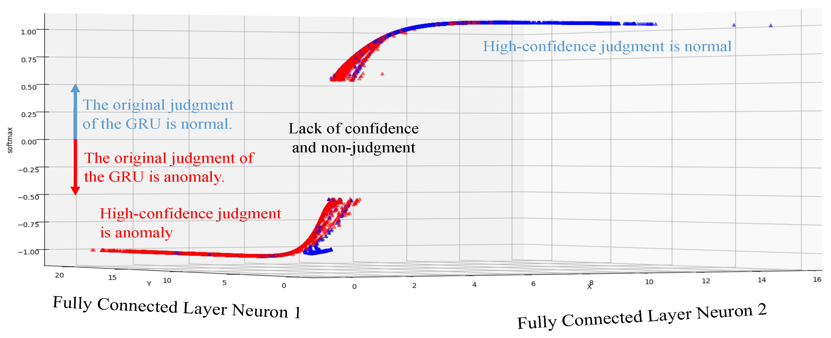
Figure 10 shows the visualization result of the GRU_3 model’s confidence judgment. The red samples and the blue samples are the actual attacks and the actual normal sample, respectively. The x and y axes are the output of two hidden layer neurons, and the z-axis is the Softmax confidence score, in which the value is between 1 and −1. The Softmax confidence score greater than 0 means that the original GRU_3 model’s judgment is normal, and the Softmax confidence score less than 0 means the judgment is abnormal. It can be found that there are many judging errors (gray blocks) in the GRU as a whole. The overall accuracy of the GRU_3 model is 78.85%, but when the confidence score is close to 1 and −1 (blue block and red block), the judging result is obviously much better. Therefore, according to the confidence threshold we set, GRU will output the samples with high confidence score, and the remaining samples with insufficient confidence will be handed over to DAE for processing. Through the data visualization in Figure 10, it can be understood that the overall under-performing model may still perform well in the judging accuracy of the high confidence interval.

4.2.3. GRU Model’s Confidence Threshold Setup

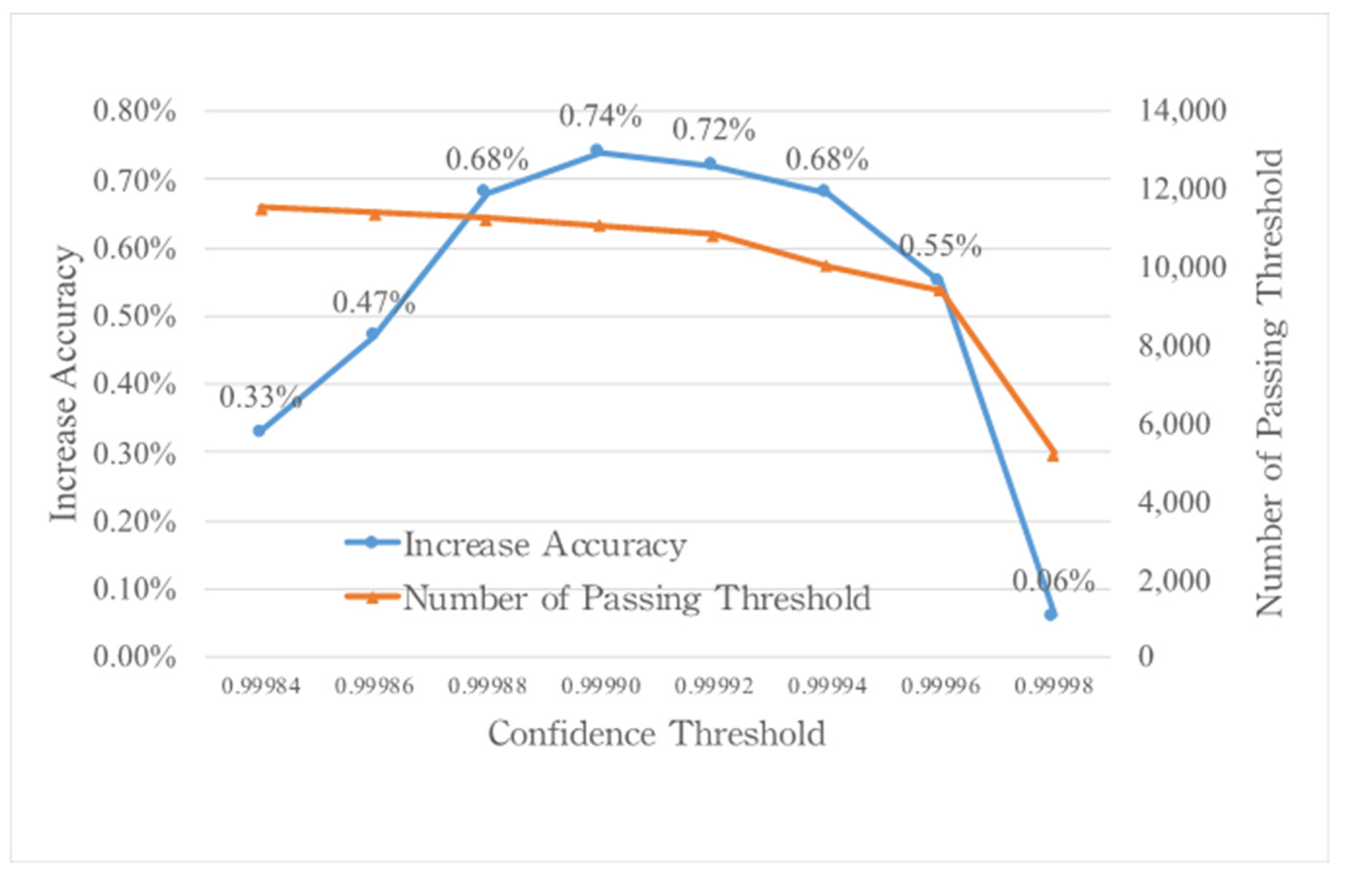
This paper tested different thresholds for the GRU model’s confidence threshold setting. We intend to observe how the adjustment of the GRU model’s confidence threshold affects the number of flows passing thresholds and how much accuracy can be improved by comparing the results of only the DAE model used. The results are shown in Figure 11. From Figure 11, we can find that when the confidence threshold is from 0.99984 to 0.99996, the accuracy of the overall structure is improved by at least 0.3%, of which 0.99990 has the best effect. The level of the threshold also directly affects the number of flows passing through the confidence threshold. The higher the threshold, the less the number of flows passes, resulting in the accuracy increasing. However, if the threshold is set too high, the number of flows passing will be reduced, and the effect of improving the accuracy will be reduced. The other extreme is that the threshold is too low. For the above reasons, we believe that the confidence threshold must be adjusted slowly from high to low in order to find an appropriate threshold.

The performance result of the GRU model with and without the confidence threshold is shown in

Table 8. The performance of GRU model with and without confidence threshold.

Model	Accuracy (%)	Precision (%)	Recall (%)	F-Measure (%)
GRU	78.85	94.05	67.09	78.32
GRU_CT	98.87	98.45	99.59	99.02

, where the confidence threshold of the GRU model is 0.99990. From the table, one can see that the accuracy of the GRU model with confidence threshold screening (GRU-CT) is better than the accuracy of the GRU model without confidence threshold screening.

4.2.4. Comparisons

Table 9. Comparison between GRU-DAE model and other approaches.

Method	Type of Learning	Accuracy (%)
RNN [5]	Supervised	83.28
1DCNN [17]	Supervised	84.29
SAE + SMR [18]	Hybrid	88.39
SAE + SVM [19]	Hybrid	84.96
AE [7]	Semi-Supervised	88.28
DAE [7]	Semi-Supervised	88.65
SAE-AE [21]	Semi-Supervised	90.17
1DCNN-DAE	Hybrid	89.95
GRU-DAE	Hybrid	90.21
GRU-DAE (best)	Hybrid	90.56

shows the comparison between the GRU-DAE model and other approaches in terms of accuracy. The accuracy of our proposed structure is 90.21%, which is better than most current methods. In addition, the best-performing of GRU-DAE model (GRU-DAE (best)) in 10 experiments can achieve 90.56% accuracy.

5. Application to SDN-Based Network Flow Anomaly Detection

Software Defined Network (SDN) is a new form of network architecture to improve the shortcomings of traditional networks, such as low scalability. The main difference between the SDN network and the traditional network is the separation of the control plane (Control Plane) and the data plane (Data Plane) of the network. The SDN controller (Controller) uses the OpenFlow protocol [27] and the OpenFlow switch (OpenFlow Switch) to communicate to manage the entire SDN network. Because the SDN network is centralized management, it is easy to collect overall network information, and it has better security than traditional networks. TATang et al. [28] proposed a NIDS based on the SDN architecture as shown in Figure 12. The network intrusion detection system module is installed on the controller side, and the SDN controller sends the ofp_flow_stats_request command to the SDN at a fixed time. All OpenFlow switches in the network request statistics about network flow characteristics. After receiving the request, the OpenFlow switch will send the ofp_flow_stats_reply command containing statistical flow characteristics information to the SDN controller for unified processing. In order to avoid the SDN controller consuming a lot of computing resources to count the characteristics of network flow, M. Latah et al. [14] selected the most suitable features for SDN by applying principal component analysis (PCA) to the NSL-KDD dataset. The selected features are shown in

Table 10. SDN-related Features on the NSL-KDD dataset after feature selection.

Feature Type	Feature Name
Basic connection features	duration, protocol_type, service, src_bytes, wrong_fragment
Flow features depending on the time connection	count, rerror_rate, diff_srv_rate
Flow features depending on the host connection	dst_host_srv_serror_rate

.

By using SDN-related features on the NSL-KDD dataset as a benchmark, we compared the experimental result of our approach applied to SDN network with several schemes experimented by M. Latah et al. [14]. The result is shown in

Table 11. Comparison between our approach and other approaches using SDN-related features of the NSL-KDD dataset as a benchmark.

Method	Accuracy (%)	Precision (%)	Recall (%)	F-Measure (%)
SVM	81.40	71.81	94.13	81.47
KNN	82.31	71.59	96.41	82.17
Random Forest	80.13	67.73	96.25	80.13
Neural Networks	74.23	59.56	92.50	72.46
AdaBoost	87.16	80.23	96.65	87.67
Decision Tree	88.74	83.24	96.50	89.38
GRU-DAE	88.33	88.80	90.97	89.87

. Although the accuracy of GRU-DAE was slightly lower than the decision tree scheme, our approach performed better than the decision tree on precision and F-measure. In particular, the precision was far ahead of other approaches.

6. Conclusions

We propose a two-stage deep learning anomaly detection structure by combining the schemes of the GRU model and DAE model. By using supervised anomaly detection with a selection mechanism to assist semi-supervised anomaly detection, the precision and accuracy of the anomaly detection system are improved. We also used the method of data visualization to understand the reasons for the insufficient accuracy of the GRU model. Moreover, we used the confidence threshold screening method to make better flow judgments. With the proposed structure, we improved the accuracy of 0.54% and precision of 0.83% of the DAE model using the NSL-KDD dataset as a benchmark, reaching an overall accuracy of 90.21%. We also applied the proposed system in the SDN environment and compared it with other IDS systems applied to the SDN environment. The results revealed that the proposed method could achieve precision of 88.8% and F-measure of 89.87%, which is better than Support Vector Machine, K-Nearest Neighbors algorithm, Decision Tree, etc. At present, this research is only tested using the NSL-KDD dataset as a benchmark. Additionally, we also found that recently several papers used UNSW-NB15 as the benchmark dataset. In the future, we will use UNSW-NB15 dataset as the benchmark dataset in our proposed structure or use the data of real network environments and make a comparison between them.