Hardware-Based Activation Function-Core for Neural Network Implementations

Abstract

Today, embedded systems (ES) tend towards miniaturization and the carrying out of complex tasks in applications such as the Internet of Things, medical systems, telecommunications, among others. Currently, ES structures based on artificial intelligence using hardware neural networks (HNNs) are becoming more common. In the design of HNN, the activation function (AF) requires special attention due to its impact on the HNN performance. Therefore, implementing activation functions (AFs) with good performance, low power consumption, and reduced hardware resources is critical for HNNs. In light of this, this paper presents a hardware-based activation function-core (AFC) to implement an HNN. In addition, this work shows a design framework for the AFC that applies a piecewise polynomial approximation (PPA) technique. The designed AFC has a reconfigurable architecture with a wordlength-efficient decoder, i.e., reduced hardware resources are used to satisfy the desired accuracy. Experimental results show a better performance of the proposed AFC in terms of hardware resources and power consumption when it is compared with state of the art implementations. Finally, two case studies were implemented to corroborate the AFC performance in widely used ANN applications.

1. Introduction

Artificial neural networks (ANNs) are an important area of artificial intelligence (AI) used to perform several tasks, such as classification [1,2,3,4], pattern recognition [5,6,7,8], communications [9,10], control systems [11,12], prediction [13,14], among others. An ANN models a biological neural network employing a collection of nodes called artificial neurons, connected by edges to transmit signals like the synapses in a brain; during its transmission, the signal value changes according to the weight of the edges, adjusted by a learning process. Each artificial neuron processes the input signals through their weighted sum and the output through an activation function (AF), which can be non-linear. The neurons in an ANN are arranged into layers, and the signal travels from the first layer (input layer) to the last layer (output layer); between these layers, the signal can travel through multiple internal layers (hidden layers). However, recent applications of ANNs, e.g., IoT, medical systems, and telecommunication, require platforms with high throughput and the capacity to execute the algorithms in real-time. An attractive solution is the development of hardware neuronal networks (HNN) in Field-Programmable Gate Arrays (FPGAs) [15,16,17,18,19,20,21]. In this regard, the FPGA-based implementation of AFs in HNN is one of the challenges for embedded system design according to recent studies; this is because the AF implementations require low hardware resources and low power consumption [1,2,5,12,22,23,24,25]. Currently, the most common non-linear functions for ANNs are the Sigmoid [11,26,27,28,29,30,31,32] ans TanhAFs [22,32,33].

For instance, ref. [4] shows a convolutional neural network (CNN) that uses the Tanh AF in each layer, and ref. [22] presents a neuroevolution of augmenting topology, which employs the Tanh and Gaussian AFs in the hidden layer and output layer, respectively. On the other hand, the exponential linear unit (ELU) and softplus AFs are used for pattern classification CNNs as shown in [23,34], respectively.

In summary, the main contributions of this paper are:

• A Sigmoid, hyperbolic tangent (Tanh), Gaussian, sigmoid linear unit (SILU), ELU, and Softplus AFs in reconfigurable hardware is designed with a piecewise polynomial approximation technique and a novel segmentation strategy.
• A wordlength-efficient hardware decoder for an activation function-core (AFC) with a reduction in power consumption in the order of 13x gains in comparison with state-of-the-art works.
• A design framework with the integration of an AFC to develop HNN applications.

The rest of the paper is organized as follows: the design methodologies for approaching AFs via PPA are presented in Section 2. The architecture and parameters for the AF hardware implementation are shown in Section 3. The hardware performance for the AFC using the proposed architecture is discussed in Section 4. The proposed AFC performance employing two case studies are presented in Section 5. Finally, conclusions are drawn in Section 6.

2. PPA Implementation Methodologies

Piecewise polynomial approximation (PPA) is a computing technique for the function approximation that offers a good trade-off between latency and memory resources. PPA splits the abscissa range into K segments, considering the $x_i$ samples on an interval $[X_L,X_H]$ and the $f\left(x_i\right)$ function. In PPA, each one of the K segments is approached by polynomial approximation as follows:

$$p_k\left(x_i\right)=a_n{x}_i^n+\cdots +a_1{x}_i+a_0,$$

(1)

where $p_k(·)$ are the polynomials corresponding to each segment, $k=1,\cdots ,K$; $a_n$ represents the polynomial coefficients, and n stands the polynomial degree. In this sense, with the aim to evaluate PPA performance, the maximum absolute error (MAE), the mean squared error (MSE), and the mean absolute error (AAE) are proposed, which are given by

$$MAE=ma{x}_{(X_L\le x_i\le X_H)}|f\left(x_i\right)-p\left(x_i\right)|,$$

(2)

$$MSE=\frac{1}{N}\sum _{i=1}^N{(f\left(x_i\right)-p\left(x_i\right))}^2,$$

(3)

$$AAE=\frac{1}{N}\sum _{i=1}^N|f\left(x_i\right)-p\left(x_i\right)|,$$

(4)

where $p(·)$ is the approximated function via PPA technique, and N is the number of $x_i$ samples. However, the signal to quantization noise ratio (SQNR) is a metric to evaluate the performance in hardware applications based on fixed-point (FxP) arithmetic. SQNR is the ratio of the signal power of interest and the quantization noise power defined as follows

$$SQN{R}_{dB}=10{\log }_{10}\frac{\frac{1}{N}{\sum }_{i=1}^{N}f{\left(x_i\right)}^2}{\frac{1}{N}{\sum }_{i=1}^N{(f\left(x_i\right)-p\left(x_i\right))}^2},$$

(5)

This study employs the PPA technique with a wordlength-efficient decoder (PPA-ED) methodology described in [35] to design the proposed AFC for HNN implementations. A comparative analysis is also provided to show the advantages of the proposed methodology with the minimax approximation [29], the simple canonical piecewise linear (SCPWL) [32], and the piecewise linear approximation computation (PLAC) [15].

2.1. Minimax Approximation

Minimax approximation minimizes the MAE across an input interval given an n-degree polynomial. This methodology takes into account the effect of rounding the coefficients to a finite wordlength, allowing a significant reduction in the size of the tables required to store the polynomial coefficients. Larkin et al. in [29] use the minimax technique to carry out the AF approximation, where a genetic algorithm is employed to obtain the segmentation, and a first-order approximation is applied:

$$a_1{x}_i+a_0,$$

(6)

where $a_1$ and $a_0$ represent the slope and the constant term for a segment, respectively; they can be computed as presented in [36]. The proposal in [29] implements a reconfigurable hardware architecture for AF approximation. However, the polynomial indexation requires the whole input wordlength, which results in an excessive use of memory resources.

2.2. Simple Canonical Piecewise Linear

According to [32], SCPWL methodology has the ability to represent the non-linear AF behavior with low complexity and high speed. In this study, the AF approximation is described by

$$c_0+\sum _{k=1}^{\mathrm{K}}{c}_k{\lambda }_k\left(x_i\right),$$

(7)

where k represents the segment index, $c_0$ is the constant term for all segments, and $c_k$ are the segment coefficients. However, the main disadvantage of SCPWL is that it requires a parallel execution of multiplications and sums to compute the contribution per segment for the polynomial evaluation of (7); consequently, the hardware resources are incremented.

2.3. Piecewise Linear Approximation Computation

PLAC is a methodology with an error-flattened segment that uses a linear approximation to improve the approximation performance under the desired MAE. This proposal splits the interval $[X_L,X_H]$ into discrete points given by

$$x_i\in \{X_L,X_L+\frac{1}{2^{iw}},X_L+\frac{2}{2^{iw}},\cdots ,X_H\},$$

(8)

where $iw$ represents the number of fractional bits for $x_i$. The number of discrete points, i.e., the number of $x_i$ samples is given by $N=(X_H-X_L)/2^{-iw}+1$, where $i=1,\cdots ,N$. The coefficients for the first-order polynomial approximation, e.g., by using (6) in the segment [$x_{\mathrm{a}},x_{\mathrm{b}}$], can be computed by

$$a_1=\frac{f\left(x_{\mathrm{b}}\right)-f\left(x_{\mathrm{a}}\right)}{x_{\mathrm{b}}-x_{\mathrm{a}}},$$

(9)

$$a_0=f\left(x_{\mathrm{a}}\right)-a_1{x}_{\mathrm{a}},$$

(10)

where [$x_{\mathrm{a}},x_{\mathrm{b}}$] ∈ $x_i$ and $x_{\mathrm{a}}<x_{\mathrm{b}}$.

The open literature presents AF hardware implementations based on PLAC; e.g., ref. [15] proposes an architecture that reduces the polynomial indexation. An advantage of PLAC is that it applies a strategy for reducing the polynomial indexation. However, disadvantages of PLAC include its use of linear approximations for approaching the AF segments that increase the segments needed to achieve the desired MAE and the need for a large amount of memory resources.

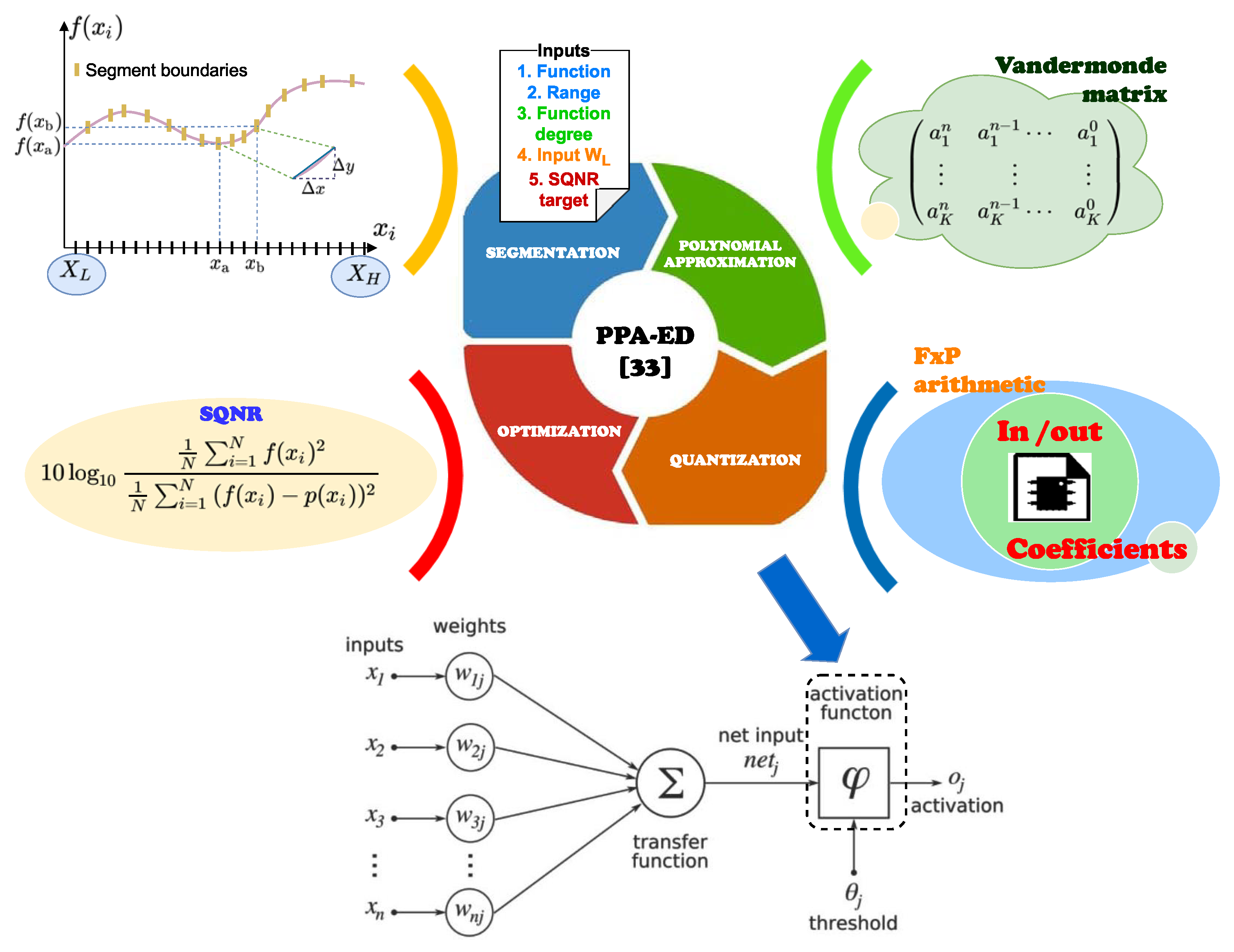
2.4. PPA with Wordlength-Efficient Decoder

The PPA-ED [35] optimizes the polynomial indexation and improves previous methodologies [15,29,32] for the hardware design of AFs according to the MAE, MSE, AAE, and SQNR metrics. This study customizes the PPA-ED to design AFCs in HNN implementations on FPGAs. Figure 1 illustrates the methodology for designing an AFC with reduced hardware and improved performance for HNN design based on the proposed method.

The adaptive segmentation, the polynomial approximation, the quantization, and the optimization processes of PPA-ED reduce hardware resources used in the design. The used methodology automatically sets up the PPA segment limits, computed as linear combinations of power-of-two, using a detection algorithm based on the function slope and the user-defined parameters in order to achieve the desired performance and optimize the polynomial indexation [35]. Likewise, PPA-ED computes the $n+1$ coefficients of n-degree for the K segments applying the Vandermonde Matrix [37]. The proposed methodology also considers a quantization process for hardware implementation that defines the FxP format required for guaranteeing the desired accuracy in terms of SQNR. All these features allow for the evaluation of the function with efficient polynomial indexing for the desired precision; consequently, a hardware architecture for the AFC with a wordlength-efficient decoder that reduces hardware resource usage is achieved.

3. AFC Hardware Implementation

The AFC implementation employs a design framework based on the proposed methodology [35]. Figure 2 shows the design framework for implementing the AFC in HNN. This study implements the AFs Sigmoid, Tanh, Gaussian, SILU, ELU, and Softplus, whose mathematical expressions are shown in

Table 1. Description of non-linear AFs for ANN.

AF	Mathematical Description	Symmetry	Evaluation Range
1. Sigmoid	$f\left(x\right)=\frac{1}{1+e^{-x}}$	$f\left(x\right)=\{\begin{array}{cc}\hfill f\left(x\right)& x\ge 0\hfill \\ \hfill 1-f\left(\right|x\left|\right)& x<0\hfill \end{array}$	$(-8,8)$
2. Tanh	$f\left(x\right)=\frac{e^x-e^{-x}}{e^x+e^{-x}}$	$f\left(x\right)=\{\begin{array}{cc}\hfill f\left(x\right)& x\ge 0\hfill \\ \hfill -f\left(\right|x\left|\right)& x<0\hfill \end{array}$	$(-8,8)$
3. Gaussian	$f\left(x\right)=e^{-x^2}$	$f\left(x\right)=\{\begin{array}{cc}\hfill f\left(x\right)& x\ge 0\hfill \\ \hfill f\left(\right|x\left|\right)& x<0\hfill \end{array}$	$(-8,8)$
4. SILU	$f\left(x\right)=\frac{x}{1+e^{-x}}$	-	$(-8,8)$
5. ELU	$f\left(x\right)=\{\begin{array}{cc}\hfill \alpha (e^x-1)& x\le 0\hfill \\ \hfill x& x>0\hfill \end{array}$	-	$(-4,4)$
6. Softplus	$f\left(x\right)=\ln (1+e^x)$	-	$(-4,4)$

. The framework consists of sequential processing stages for the AFC custom design on FxP arithmetic and its integration in HNN implementations. The workflow describes the design steps for a HW design on FPGA devices.

The first stage of the framework is related to the PPA-ED configuration, e.g., polynomial degree, SQNR target, and FxP wordlength requirements. The second stage is the PPA segmentation, which calculates the optimum number of segments and the required coefficients for the function evaluation with the desired accuracy.

In the third stage, the PPA-ED optimizes the AFC in an iterate way. The fourth stage generates the custom Verilog design of the AFC. The last stage corresponds to the HNN design, which is obtained by using the designed AFC into a ANN model.

The AFC implementation uses the proposed reconfigurable and wordlength-efficient hardware architecture shown in Figure 3, where ${\mathrm{a}}_n$ represents the polynomial coefficients, $\mathrm{x}$ is the input represented on FxP, and $\mathrm{f}\left(\mathrm{x}\right)$ is the output of the evaluated function. Figure 4 depicts the function evaluator block for the proposed architecture, which computes a second-order AF evaluation on FxP arithmetic by employing Horner’s rule [36]. The LUT block contains the coefficients for AF evaluation, and the address decoder unit indexes the LUT according to the bits_agu frame shown in Figure 5. The LUT address has a width of $\mathrm{L}=\lceil {log}_2\left(\mathrm{K}\right)\rceil$ bits, where K represents the number of segments and $\lceil ·\rceil$ stands for the ceil function. The proposed AFC architecture considers and exploits the AF symmetry to reduce the hardware resources.

Table 2. FxP format for implementing AFC in HNN.

Activation Function	Input/Output FxP Format Q(${\mathit{W}}_{\mathit{L}}$,QFW,s)	Coefficients FxP Format Q(${\mathit{W}}_{{\mathit{L}}_{\mathit{C}}}$,QFC,s)
1.      Sigmoid	(16,10,s)	(16,15,s)
2.      Tanh	(16,10,s)	(16,14,s)
3.      Gaussian	(16,10,s)	(16,14,s)
4.      SILU	(16,11,s)	(16,13,s)
5.      ELU	(16,12,s)	(16,15,s)
6.      Softplus	(16,12,s)	(16,15,s)

shows the FxP format corresponding to the input/output values and the polynomial coefficients. The FxP signed format Q($W_L$,QFW,s) considers a wordlength $W_L$ and the fractional bits QFW. In the case of the polynomial coefficients, the FxP signed format Q($W_{L_C}$,QFC,s) considers a $W_{L_C}$ wordlength and the fractional bits QFC.

4. Experimental Results and Discussion

To verify the proposed reconfigurable architecture for the AFC (see Figure 3), the selected AFs (see Table 1 and Table 2) were approximated employing the proposed methodology in Section 2.4. Likewise, the implementation for the AFC architecture was according to the hardware specification and the polynomial coefficients shown in Table 2,

Table 3. Floating-point and fixed-point coefficients for implementing Sigmoid AF in HNN.

Segment Number	Segment Boundaries	Format	${\mathbf{a}}_2$	${\mathbf{a}}_1$	${\mathbf{a}}_0$
1	[0 1.5)	★	$-0.0364$	0.2685	0.4981
		☐	0xfb55	0x225f	0x3fc2
2	[1.5 3.5)	★	$-0.03$	0.2243	0.551
		☐	0xfc29	0x1cb4	0x4687
3	[3.5 4.5)	★	$-0.0086$	0.0873	0.7712
		☐	0xfee4	0x0b2b	0x62b8
4	[4.5 8.0)	★	$-0.0012$	0.0174	0.9356
		☐	0xffd9	0x023b	0x77c0

★ Floating-point. ☐ Fixed-point in hexadecimal notation.

,

Table 4. Floating-point and fixed-point coefficients for implementing Tanh AF in HNN.

Segment Number	Segment Boundaries	Format	${\mathbf{a}}_2$	${\mathbf{a}}_1$	${\mathbf{a}}_0$
1	[0 1)	★	$-0.3269$	1.0968	$-0.0055$
		☐	0xeb14	0x4631	0xffa5
2	[1 2)	★	$-0.1691$	0.7027	0.2318
		☐	0xf52d	0x2cf8	0x0ed5
3	[2 3.5)	★	$-0.0189$	0.1242	0.7933
		☐	0xfeca	0x07f2	0x32c4
4	[3.5 8)	★	$-0.0001$	0.0019	0.9939
		☐	0xfffd	0x001f	0x3f9b

★ Floating-point. ☐ Fixed-point in hexadecimal notation.

,

Table 5. Floating-point and fixed-point coefficients for implementing Gaussian AF in HNN.

Segment Number	Segment Boundaries	Format	${\mathbf{a}}_2$	${\mathbf{a}}_1$	${\mathbf{a}}_0$
1	[0 0.50)	★	$-0.9458$	$-0.0065$	1.0001
		☐	0xc378	0xff96	0x4001
2	[0.50 1.00)	★	$-0.5053$	$-0.2634$	1.0377
		☐	0xdfa9	0xef23	0x426a
3	[1.00 1.25)	★	0.1554	$-1.0796$	1.2914
		☐	0x09f2	0xbae8	0x52a5
4	[1.25 1.75)	★	0.4353	$-1.6126$	1.5452
		☐	0x1bdc	0x98ca	0x62e5
5	[1.75 2.50)	★	0.3366	$-1.3284$	1.3409
		☐	0x158a	0xaafc	0x55d1
6	[2.50 3.75)	★	0.1318	$-0.6063$	0.7035
		☐	0x0870	0xd932	0x2d05
7	[3.75 5.25)	★	0.0157	$-0.0895$	0.1281
		☐	0x0100	0xfa45	0x0833
8	[5.25 8.00)	★	0	$-0.0001$	0.0002
		☐	0x0000	0xffff	0x0002

★ Floating-point. ☐ Fixed-point in hexadecimal notation.

,

Table 6. Floating-point and fixed-point coefficients for implementing SILU AF in HNN.

Segment Number	Segment Boundaries	Format	${\mathbf{a}}_2$	${\mathbf{a}}_1$	${\mathbf{a}}_0$
1	[−8 −4.5)	★	−0.0045	−0.0686	−0.2641
		☐	0xffda	0xfdcd	0xf78c
2	[−4.5 −2)	★	−0.0149	−0.174	−0.53002
		☐	0xff86	0xfa6e	0xef09
3	[−2 −1)	★	0.0798	0.2053	−0.1453
		☐	0x028d	0x0691	0xfb5a
4	[−1 0.5)	★	0.2329	0.4997	0.0015
		☐	0x0773	0x0ffd	0x000c
5	[0.5 2)	★	0.115	0.6885	−0.0689
		☐	0x03ae	0x1608	0xfdcb
6	[2 3.5)	★	−0.0095	1.1447	−0.4912
		☐	0xffb1	0x24a1	0xf047
7	[3.5 6)	★	−0.0115	1.1431	−0.4611
		☐	0xffa1	0x2494	0xf13e
8	[6 8]	★	−0.0024	1.039	−0.1635
		☐	0xffec	0x213f	0xfac4

★ Floating-point. ☐ Fixed-point in hexadecimal notation.

,

Table 7. Floating-point and fixed-point coefficients for implementing ELU AF in HNN.

Segment Number	Segment Boundaries	Format	${\mathbf{a}}_2$	${\mathbf{a}}_1$	${\mathbf{a}}_0$
1	[−4 −2.5)	★	0.004	0.0345	−0.1227
		☐	0x0084	0x046c	0xf04a
2	[−2.5 −1.5)	★	0.0138	0.0831	−0.0621
		☐	0x01c4	0x0aa1	0xf80e
3	[−1.5 −0.5)	★	0.0375	0.1507	−0.0133
		☐	0x04cd	0x134a	0xfe4d
4	[−0.5 0)	★	0.0783	0.1961	−0.0001
		☐	0x0a05	0x191a	0xfffc

★ Floating-point. ☐ Fixed-point in hexadecimal notation.

and

Table 8. Floating-point and fixed-point coefficients for implementing Softplus AF in HNN.

Segment Number	Segment Boundaries	Format	${\mathbf{a}}_2$	${\mathbf{a}}_1$	${\mathbf{a}}_0$
1	[−4 −2)	★	0.0238	0.1948	0.4184
		☐	0x030c	0x18ef	0x358e
2	[−2 0 )	★	0.0969	0.472	0.68844
		☐	0x0c67	0x3c68	0x581e
3	[0 2)	★	0.0969	0.528	0.68844
		☐	0x0c67	0x4397	0x581e
4	[2 4]	★	0.0238	0.8052	0.4184
		☐	0x030c	0x6710	0x358e

★ Floating-point. ☐ Fixed-point in hexadecimal notation.

. As was mentioned in the hardware design framework, Verilog is the hardware description language for implementing the AFC, synthesized on a Xilinx Artix-7 xc7a100t-2csg324 FPGA device.

Table 9. Performance comparison for the implemented AFs based on minimax approximation and PPA-ED methodologies.

$\mathbf{x}$ ∈ Q(14,10,s),   $\mathbf{f}\left(\mathbf{x}\right)$ ∈ Q(12,10,s)
Function	Proposal	Segments	SQNR [dB]	Range	MAE	AAE
Sigmoid	Larkin * [29]	4	NA	$(-8,8)$	$4.7\times {10}^{-3}$	$2.4\times {10}^{-3}$
		6	NA		$2.3\times {10}^{-3}$	$1.2\times {10}^{-3}$
	PPA-ED **	4	59.49		$2.1\times {10}^{-3}$	$8.3\times {10}^{-4}$
Tanh	Larkin * [29]	4	NA	$[0,8)$	$9.5\times {10}^{-3}$	$2.4\times {10}^{-3}$
	PPA-ED **	4	53.40		$5.9\times {10}^{-3}$	$1.2\times {10}^{-3}$
		3	50.60		$10.7\times {10}^{-3}$	$1.7\times {10}^{-3}$

* First order polynomial. ** Second order polynomial.

,

Table 10. Performance comparison for the implemented AFs based on SCPWL and PPA-ED methodologies.

$\mathbf{x}$, $\mathbf{f}\left(\mathbf{x}\right)$ ∈ Q(16,10,s)
Function	Proposal	Segments	SQNR [dB]	Range	MAE	MSE
Sigmoid	Hussein * [32]	9	NA	$(-8,8)$	$5.2\times {10}^{-3}$	$1.8\times {10}^{-6}$
	PPA-ED **	4	56.76		$2.1\times {10}^{-3}$	$9.2\times {10}^{-7}$
Tanh	Hussein * [32]	9	NA	$(-8,8)$	$15.4\times {10}^{-3}$	$1.2\times {10}^{-5}$
	PPA-ED **	4	53.55		$5.9\times {10}^{-3}$	$3.9\times {10}^{-6}$
Gaussian	Hussein * [32]	9	NA	$(-8,8)$	$7.0\times {10}^{-3}$	$1.4\times {10}^{-5}$
	PPA-ED **	8	49.48		$1.7\times {10}^{-3}$	$8.9\times {10}^{-7}$
	PPA-ED	6	41.96		$3.9\times {10}^{-3}$	$5.23\times {10}^{-6}$

* First order polynomial. ** Second order polynomial.

,

Table 11. Performance comparison for the implemented AFs based on PLAC and PPA-ED methodologies.

$\mathbf{x}$, $\mathbf{f}\left(\mathbf{x}\right)$ ∈ Q(8,8,ns)
Function	Proposal *	Segments	Range	SQNR [dB]	MAE
Sigmoid	Dong [15]	2	[0,1)	NA	$5.65\times {10}^{-3}$
	PPA-ED	2		48.22	$3.91\times {10}^{-3}$
Tanh	Dong [15]	4	[0,1)	NA	$5.55\times {10}^{-3}$
	PPA-ED	4		46.03	$3.91\times {10}^{-3}$

* First order polynomial.

,

Table 12. Hardware performance for the implemented PPA-ED-based AFC.

Function	Range	SQNR	MAE	AAE	Power Consumption ${}^{*}$ [mW]
Sigmoid	$(-8,8)$	56.76	$2.1\times {10}^{-3}$	$9.2\times {10}^{-7}$	0.82
Tanh	$(-8,8)$	53.55	$5.9\times {10}^{-3}$	$3.9\times {10}^{-6}$	0.88
Gaussian	$(-8,8)$	53.55	$5.9\times {10}^{-3}$	$3.9\times {10}^{-6}$	0.88
ELU	$(-4,4)$	78.73	$5.6\times {10}^{-4}$	$1.1\times {10}^{-4}$	0.53
SILU	$(-8,8)$	60.14	$7.9\times {10}^{-3}$	$2.6\times {10}^{-3}$	0.96
Softplus	$(-4,4)$	59.50	$5.2\times {10}^{-3}$	$1.4\times {10}^{-3}$	0.66

* Frequency 40 MHz.

,

Table 13. Power consumption comparison for Sigmoid AF.

Proposal	Segments	MAE	AAE	Frequency [MHz]	Average Power [mW]
Larkin [29]	8	$1.3\times {10}^{-3}$	$0.9\times {10}^{-3}$	40	17
PPA-ED-based	5	$1.2\times {10}^{-3}$	$3.6\times {10}^{-4}$	40	1.02
AFC				50	1.27

and

Table 14. Hardware resource usage for the PPA-ED-based AFCs.

HW Resources	Consumption by Function							Available	Utilization
	Sigmoid	Tanh	Gaussian	ELU	SILU	Softplus			%
Slice register	1	1	0	16	0	0	Out of	126,800	0%
Slice LUTs	76	78	93	28	54	22	Out of	63,400	0%
IOBs	33						Out of	210	15%
BUFG/
BUFGCTRLs	1						Out of	32	3%
DSP48E1s	2						Out of	240	0%

show the performance comparisons for the PPA-ED-based AFC implemented. In this sense, Table 9 shows the AFC performance results based on the methodologies minimax approximation [29] and PPA-ED, for the Sigmoid and Tanh AFs. The input/output Fxp representations were configured according to [29] for a fair comparison. As can be seen, for the Sigmoid AF with 4 segments, the proposed methodology improves [29], reducing the MAE in 55.3% and the AAE in 65.4%. Even increasing the segments to 6 in [29], PPA-ED reduces the MAE in 8.7% and the AAE in 30.8%. Likewise, for the case of Tanh AF with 4 segments, MAE is reduced in 37.9% and the AAE in 50%.

In order to compare the performance between the PPA-ED-based AFC and SCPWL implementation [32], the proposed methodology was configured with a number of segments to provide a similar number of polynomial coefficients according to the implementation results reported in [32]. Likewise, the AFC architectures were configured with the same FxP requirements. Table 10 shows the AFC performance comparison implemented via PPA-ED and SCPWL. As the implementation results show, the proposed method reduces the MAE in 59% and 61%, and the MSE in 48% and 67%, for the Sigmoid and Tanh AFs, respectively. Likewise, comparison results for architectures designed via PLAC [15] and PPA-ED methodologies can be observed in Table 11. In this case, the PPA-ED-based AFC reduces the MAE in 30.79% and 29.54% for Sigmoid and Tanh AFs, respectively.

Table 12 shows the power consumption results of the PPA-ED-based AFC designs obtained by Xilinx Power Analyzer. These results are outstanding compared with the other proposals; e.g., Table 13 shows the power comparison results when implementing the Sigmoid AF via Minimax approximation [29]. As can be seen, the AFC implemented via PPA-ED improves the average power consumption at least 13x. Finally, Table 14 shows the hardware resources used for implementing PPA-ED-based AFCs according to the proposed design framework. The AFCs achieve a maximum work frequency of 51.71 MHz, 53.69 MHz, 59.45 MHz, 57.87 MHz, 57.64 MHz, and 57.74 MHz for Sigmoid, Tanh, Gaussian, ELU, SILU, and Softplus, respectively.

As can be seen in Table 9, Table 10, Table 11, Table 12, Table 13 and Table 14, experimental results have shown a better performance of the PPA-ED methodology to implement AFCs in terms of MAE, MSE, AAE, SQNR, and power consumption, achieving a power reduction of at least 13x for the Sigmoid AF.

5. Hardware Neural Networks: Case Studies

Two case studies on ANN applications support the implemented PPA-ED-based AFCs, which were selected because ANNs are continuously under research and the development of devices considering reduced hardware has relevance for the applications of embedded systems based on HNNs [38,39,40,41,42,43]. The efficiency of the proposed PPA-ED methodology is demonstrated on an FPGA-based accelerator(AFC), which employs minimal hardware resources. Here, under the co-simulation paradigm, the validation of the proposed design was conducted. In this sense, an FxP-based reference ANN (golden model) was developed using Matlab/Simulink, and the results were compared with a design according to the proposed design framework for HNNs (see Figure 2).

The first case study is related to the implementation of a digital classification neural network that uses an ELU AFC. The digit classification neural network identifies digits between zero and nine. The second case study uses a Tanh AFC to implement a breast cancer neural network application, the aim of which is to classify the cancers as either benign or malignant depending on the characteristics of sample biopsies.

5.1. Digit Classification

The digital classification applied the MNIST database of handwritten digits with a training matrix of 60,000 rows × 785 columns [44]. Each row of the matrix represents one digit of the database containing a label and image of 28 × 28 pixel grayscale; the digit label is in the first column, and the remaining 784 columns have the pixel information.

Figure 6 shows the implemented digit classification ANN structure. In this case study, 50 epochs were computed for the training process. The simulation results show that the PPA-ED-based AFC has an error of 0.01%, identifying 97.2% of the samples, which converge to the results generated by the FxP-based reference ANN (golden model).

5.2. Breast Cancer Detection

The case study on breast cancer detection applied the data set provided by Matlab, with an input matrix with 9 rows × 699 columns [45]. The columns represent the biopsies with the attributes contained in the rows. The breast cancer detection ANN structure has ten neurons in one hidden layer and two in the output layer. The hidden layer employs the Tanh AFC. This ANN computed 27 epochs for the training process.

The performance comparison for the breast cancer ANN is shown in Figure 7, in which the ANN placed at the top corresponds to the ANN implemented by Simulink blocks, and the ANN at the bottom side corresponds to the proposed PPA-ED-based design under co-simulation. Both models achieved an accuracy of 97.80%, which demonstrates the effectiveness of the proposed model.

6. Conclusions

In this paper, the use of the PPA-ED methodology to implement AFC in HNN was presented. The proposal is focused on the AFC implementation providing an efficient architecture and configuration parameters; however, the tune on of the ANN hyperparameters is offline. In order to reach this aim, a reconfigurable and wordlength-efficient decoder for the AFC hardware architecture was proposed. This architecture performs a second-order polynomial function evaluation to approach the selected AFs. In this sense, a hardware neural network framework was introduced, which allows verifying the proposed PPA-ED-based design in terms of the MAE, AAE, and SQNR metrics. Likewise, a comparative analysis was provided to show the advantages of the PPA-ED in contrast to the minimax approximation, SCPWL, and PLAC methodologies. Additionally, two case studies were presented to corroborate the AFC in widely used ANN applications. Finally, experimental results have shown a better performance of the PPA-ED methodology to implement AFCs in terms of MAE, AAE, SQNR, and power consumption, achieving a power reduction of at least 13x for the Sigmoid AF. AFC performance analysis on floating-point arithmetic is considered for further works.

References

1. Viswanath, K.; Gunasundari, R. VLSI Implementation and Analysis of Kidney Stone Detection from Ultrasound Image by Level Set Segmentation and MLP-BP ANN Classification; Advances in Intelligent Systems and Computing; Springer: New Delhi, India, 2016; Volume 394. [Google Scholar] [CrossRef]
2. Sarić, R.; Jokić, D.; Beganović, N.; Gurbeta, P.; Badnjević, A. FPGA-based real-time epileptic seizure classification using Artificial Neural Network. Biomed. Signal Process. Control 2020, 62, 102106. [Google Scholar] [CrossRef]
3. Tong, D.L.; Mintram, R. Genetic Algorithm-Neural Network (GANN): A study of neural network activation functions and depth of genetic algorithm search applied to feature selection. Int. J. Mach. Learn. Cybern. 2010, 1, 75–87. [Google Scholar] [CrossRef]
4. Abdelouahab, K.; Pelcat, M.; Berry, F. Why TanH can be a Hardware Friendly Activation Function for CNNs. In Proceedings of the 11th International Conference on Distributed Smart Cameras, Stanford, CA, USA, 5–7 September 2017. [Google Scholar]
5. Medus, L.; Iakymchuk, T.; Frances, V.; Bataller, M.; Rosado, M. A Novel Systolic Parallel Hardware Architecture for the FPGA Acceleration of Feedforward Neural Networks. IEEE Access 2019, 7, 76084–76103. [Google Scholar] [CrossRef]
6. Zhang, L. Artificial neural network model-based design and fixed-point FPGA implementation of hénon map chaotic system for brain research. In Proceedings of the 2017 IEEE XXIV International Conference on Electronics, Electrical Engineering and Computing (INTERCON), Cusco, Peru, 15–18 August 2017. [Google Scholar]
7. Narvekar, M.; Fargose, P.; Mukhopadhyay, D. Weather Forecasting Using ANN with Error Backpropagation Algorithm, Proceedings of the International Conference on Data Engineering and Communication Technology; Advances in Intelligent Systems and Computing; Springer: Singapore, 2017. [Google Scholar] [CrossRef]
8. Libano, F.; Rech, P.; Tambara, L.; Tonfat, J.; Kastensmidt, F. On the Reliability of Linear Regression and Pattern Recognition Feedforward Artificial Neural Networks in FPGAs. IEEE Trans. Nucl. Sci. 2018, 65, 288–295. [Google Scholar] [CrossRef]
9. Mahdi, S.Q.; Gharghan, S.K.; Hasan, M.A. FPGA-Based neural network for accurate distance estimation of elderly falls using WSN in an indoor environment. Measurement 2021, 167, 108276. [Google Scholar] [CrossRef]
10. Louliej, A.; Jabrane, Y.; Zhu, W.P. Design and FPGA implementation of a new approximation for PAPR reduction. AEU-Int. J. Electron. Commun. 2018, 94, 253–261. [Google Scholar] [CrossRef]
11. Hartmann, N.B.; Dos-Santos, R.C.; Grilo, A.P.; Vieira, J.C.M. Hardware Implementation and Real-Time Evaluation of an ANN-Based Algorithm for Anti-Islanding Protection of Distributed Generators. IEEE Trans. Ind. Electron. 2018, 65, 5051–5059. [Google Scholar] [CrossRef]
12. Hultmann, A.; Muñoz, D.; Llanos, C.; Dos-Santos, C. Efficient hardware implementation of radial basis function neural network with customized-precision floating-point operations. Control. Eng. Pract. 2017, 60, 124–132. [Google Scholar] [CrossRef]
13. Tng, S.S.; Le, N.Q.K.; Yeh, H.Y.; Chua, M.C.H. Improved Prediction Model of Protein Lysine Crotonylation Sites Using Bidirectional Recurrent Neural Networks. J. Proteome Res. 2021. [Google Scholar] [CrossRef]
14. Le, N.Q.; Nguyen, B.P. Prediction of FMN Binding Sites in Electron Transport Chains based on 2-D CNN and PSSM Profiles. IEEE/ACM Trans. Comput. Biol. Bioinform. 2019. [Google Scholar] [CrossRef] [PubMed]
15. Dong, H. PLAC: Piecewise Linear Approximation Computation for All Nonlinear Unary Functions. IEEE Trans. Very Large Scale Integr. (VLSI) Syst. 2020, 28, 2014–2027. [Google Scholar] [CrossRef]
16. Parra, D.; Camargo, C. A Systematic Literature Review of Hardware Neural Networks. In Proceedings of the 2018 IEEE 1st Colombian Conference on Applications in Computational Intelligence (ColCACI), Medellin, Colombia, 16–18 May 2018. [Google Scholar] [CrossRef]
17. Raut, G.; Rai, S.; Vishvakarma, S.K.; Kumar, A. A CORDIC Based Configurable Activation Function for ANN Applications. In Proceedings of the 2020 IEEE Computer Society Annual Symposium on VLSI, Limassol, Cyprus, 6–8 July 2020; pp. 78–83. [Google Scholar] [CrossRef]
18. Yang, T. Design Space Exploration of Neural Network Activation Function Circuits. IEEE Trans. Comput.-Aided Des. Integr. Circuits Syst. 2019, 38, 1974–1978. [Google Scholar] [CrossRef] [Green Version]
19. Xie, Y.; Joseph RA, N.; Hu, Z.; Huang, S.; Fan, Z.; Joler, M. A Twofold Lookup Table Architecture for Efficient. IEEE Trans. Very Large Scale Integr. (VLSI) Syst. 2020, 28, 2540–2550. [Google Scholar] [CrossRef]
20. Cococcioni, M.; Rossi, F.; Ruffaldi, E.; Saponara, S. Fast Approximations of Activation Functions in Deep Neural Networks when using Posit Arithmetic. Sensors 2020, 20, 1515. [Google Scholar] [CrossRef] [PubMed] [Green Version]
21. Bouguezzi, S.; Fredj, H.B.; Belabed, T.; Valderrama, C.; Faiedh, H.; Souani, C. An Efficient FPGA-Based Convolutional Neural Network for Classification: Ad-MobileNet. Electronics 2021, 10, 2272. [Google Scholar] [CrossRef]
22. Papavasileiou, E.; Jansen, B. The importance of the activation function in NeuroEvolution with FS-NEAT and FD-NEAT. In Proceedings of the 2017 IEEE Symposium Series on Computational Intelligence (SSCI), Honolulu, HI, USA, 27 November–1 December 2017. [Google Scholar] [CrossRef]
23. Qian, S.; Liu, H.; Liu Ch Wu, S.; Wong, H. Adaptive activation functions in convolutional neural networks. Neurocomputing 2018, 272, 204–212. [Google Scholar] [CrossRef]
24. Mitra, S.; Chattopadhyay, P. Challenges in implementation of ANN in embedded system. In Proceedings of the 2016 International Conference on Electrical, Electronics, and Optimization Techniques (ICEEOT), Chennai, India, 3–5 March 2016; pp. 1794–1798. [Google Scholar]
25. Kim, J.; Kim, J.; Kim, T.H. AERO: A 1.28 MOP/s/LUT Reconfigurable Inference Processor for Recurrent Neural Networks in a Resource-Limited FPGA. Electronics 2021, 10, 1249. [Google Scholar] [CrossRef]
26. Dlugosz, Z.; Dlugosz, R. Nonlinear Activation Functions for Artificial Neural Networks Realized in Hardware. In Proceedings of the 25th International Conference “Mixed Design of Integrated Circuits and Systems”, Gdynia, Poland, 21–23 June 2018. [Google Scholar] [CrossRef]
27. Armato, A.; Fanucci, L.; Scilingo, E.; De Rossi, D. Low-error digital hardware implementation of artificial neuron activation functions and their derivative. Microprocess. Microsyst. 2011, 35, 557–567. [Google Scholar] [CrossRef]
28. Tsmots, I.; Skorokhoda, O.; Rabyk, V. Hardware Implementation of Sigmoid Activation Functions using FPGA. In Proceedings of the 2019 IEEE 15th International Conference on the Experience of Designing and Application of CAD Systems (CADSM), Polyana, Ukraine, 26 February–2 March 2019; pp. 34–38. [Google Scholar] [CrossRef]
29. Larkin, D.; Kinane, A.; Muresan, V.; O’Connor, N. An Efficient Hardware Architecture for a Neural Network Activation Function Generator. Adv. Neural Netw. 2006, 3973, 1319–1327. [Google Scholar] [CrossRef] [Green Version]
30. Zhang, L. Implementation of Fixed-point Neuron Models with Threshold, Ramp and Sigmoid Activation Functions. IOP Conf. Ser. Mater. Sci. Eng. 2017, 224, 012054. [Google Scholar] [CrossRef] [Green Version]
31. Nguyen, V.; Luong, T.; Le Duc, H.; Hoang, V. An Efficient Hardware Implementation of Activation Using Stochastic Computing for Deep Neural Networks. In Proceedings of the 2018 IEEE 12th International Symposium on Embedded Multicore/Many-core Systems-on-Chip, Hanoi, Vietnam, 12–14 September 2018; pp. 233–236. [Google Scholar] [CrossRef]
32. Hussein, M.H.; Al-Rikabi Mohannad, A.M.; Al-Ja’afari Ameer, H.A.; Saif, H.A. Generic model implementation of deep neural network activation functions using GWO-optimized SCPWL model on FPGA. Microprocess. Microsyst. 2020, 77, 103141. [Google Scholar] [CrossRef]
33. Zhengbo, C.; Lei, T.; Zuoning, C. Research and design of activation function hardware implementation methods. J. Phys. Conf. Ser. 2020, 1684, 012111. [Google Scholar] [CrossRef]
34. Guoxin, W.; Xiuli, L.; Zhanglei, J.; Ruxiang, H. Dongba classical ancient books image classification method based on ReN-Softplus convolution residual neural network. In Proceedings of the 14th IEEE International Conference on Electronic Measurement & Instruments (ICEMI), Changsha, China, 1–3 November 2019; pp. 398–404. [Google Scholar] [CrossRef]
35. González, G.; Longoria, O.; Carrasco, R. An Optimization Methodology for Designing Hardware-Based Function Evaluation Modules with Reduced Complexity. Circuits Syst. Signal Process. 2021, in press. [Google Scholar] [CrossRef]
36. Muller, J.-M. Elementary Functions: Algorithms and Implementation, 3rd ed.; Birkhäuser: Boston, MA, USA, 2016. [Google Scholar]
37. Lancaster, P.; Tismenetsky, M. The Theory of Matrices: With Applications, 2nd ed.; Elsevier: San Diego, CA, USA, 1985. [Google Scholar] [CrossRef]
38. Ahlawat, S.; Choudhary, A.; Nayyar, A.; Singh, S.; Yoon, B. Improved Handwritten Digit Recognition Using Convolutional Neural Networks (CNN). Sensors 2020, 20, 3344. [Google Scholar] [CrossRef]
39. Alwzwazy, H.A.; Albehadili, H.M.; Alwan, Y.S.; Islam, N.E. Handwritten digit recognition using convolutional neural networks. Int. J. Innov. Res. Comput. Commun. Eng. 2016, 4, 1101–1106. [Google Scholar]
40. Ali, S.; Shaukat, Z.; Azeem, M. An efficient and improved scheme for handwritten digit recognition based on convolutional neural network. SN Appl. Sci. 2019, 1, 1125. [Google Scholar] [CrossRef] [Green Version]
41. Ting, F.F.; Tan, Y.J.; Sim, K.S. Convolutional neural network improvement for breast cancer classification. Expert Syst. Appl. 2019, 120, 103–115. [Google Scholar] [CrossRef]
42. Alom, M.Z.; Yakopcic, C.; Nasrin, M.S. Breast Cancer Classification from Histopathological Images with Inception Recurrent Residual Convolutional Neural Network. J. Digit. Imaging 2019, 32, 605–617. [Google Scholar] [CrossRef] [PubMed] [Green Version]
43. Toğaçar, M.; Özkurt, K.B.; Ergen, B.; Cömert, Z. BreastNet: A novel convolutional neural network model through histopathological images for the diagnosis of breast cancer. Phys. A Stat. Mech. Appl. 2020, 545, 123592. [Google Scholar] [CrossRef]
44. Langelaar, J. MNIST Neural Network Training and Testing; MATLAB Central File Exchange; Available online: https://www.mathworks.com/matlabcentral/fileexchange/73010-mnist-neural-network-training-and-testing (accessed on 20 September 2021).
45. Murphy, P.M.; Aha, D.W. UCI Repository of Machine Learning Databases. Available online: http://www.ics.uci.edu/~mlearn/MLRepository.html (accessed on 25 September 2021).
Figure 1. Methodology for designing the AFC.
Electronics 11 00014 g001
Figure 2. Design framework for implementing AFC in HNN.
Electronics 11 00014 g002
Figure 3. Proposed hardware architecture for implementing the AFC.
Electronics 11 00014 g003
Figure 4. Function evaluator for the implemented AFC.
Electronics 11 00014 g004
Figure 5. Input data structure, x .
Electronics 11 00014 g005
Figure 6. Digit classification ANN structure.
Electronics 11 00014 g006
Figure 7. Breast cancer detection ANN performance comparison.
Electronics 11 00014 g007